COMPARISON OF FIVE HEALTH-RELATED QUALITY-OF-LIFE INDEXES USING ITEM RESPONSE THEORY ANALYSIS

Abstract

Background

Five health-related quality-of-life (HRQoL) indexes—EQ-5D, HUI2, HUI3, QWB-SA, and SF-6D—are each used to assign community-based utility scores to health states, although these scores differ.

Objective

The authors transform these indexes to a common scale to understand their interrelationships.

Methods

Data were from the National Health Measurement Study, a telephone survey of 3844 US adults. The 5 indexes were analyzed using item response theory analysis to estimate scores on an underlying construct of summary health, θ. Unidimensionality was evaluated using nonlinear principal components analysis. Index scores were plotted against the estimated scores on the common underlying construct. In addition, scores on the Health and Activities Limitation Index (HALex), the Centers for Disease Control and Prevention Healthy Days questions, and self-rated health on a 5-category scale ranging from excellent to poor were plotted.

Results

SF-6D and QWB-SA are nearly linear across the range of θ, but with a shallow slope; EQ-5D, HUI2, and HUI3 are linear with steep slope from low θ (poor health) into mid-range of θ, then approximately linear with a less steep slope for higher θ (health just below to well above average) although the inflection points differ by index.

Conclusion

Simple linear functions may serve as crosswalks among these indexes only for lower health states albeit with low precision. Ceiling effects make crosswalks among most of the indexes ill specified above a certain level of health. Although each index measures generic health on a utility scale, these indexes are not identical but are relatively simply, if imprecisely, related.

INTRODUCTION

Five health-related quality-of-life (HRQoL) indexes—the EuroQoL EQ-5D (EQ-5D), Health Utilities Index Mark 2 and Mark 3 (HUI2, HUI3), Quality of Well-Being Index Self-Administered Version (QWB-SA), and the SF-6D (a utility-valued summary scale based on data from the SF-36v2™)—are commonly used to assign community-based utility scores to health states for summarizing patients’ health in clinical studies, for population health monitoring, and for cost-effectiveness analysis. Although each of these indexes was constructed as a summary measure of generic health using a score of 1.0 to represent best health and 0.0 to represent being dead, it is well-known that their scales have different ranges and that they may assign different HRQoL utility scores to the same person. An important problem is how to compare results obtained using one of these 5 measures to results from another.

The primary purpose of this article is to gain a better understanding of how the scales for each of these 5 indexes compare to one another and to suggest next steps in the process of developing “crosswalks” among the indexes. Although many studies have collected data using 2 or more of these measures and then compared them, most such comparisons have consisted of comparing percentages of cases at the ceiling or floor, correlations among the measures, mean scores, mean change scores, or the ability to discriminate subgroups such as people with v. without a particular disease (see, e.g., Houle and Berthelot [1], Kaplan, Groessl, Sengupta and others [2], Luo, Chew, Fong and others [3], Luo, Johnson, Shaw and others [4], Pickard, Johnson, Feeny [5], and Davison, Jhangri, Feeny [6]).

We take a different approach here. The National Health Measurement Study (NHMS) administered the 5 indexes simultaneously to a cross-sectional sample of older US adults [7]. We use these data to locate subjects on a latent continuum of summary health defined jointly by the 5 measures and then compare the relationships between the native scales and this underlying construct. In this manner we gain a measurement-based perspective on how, relative to one another, the different indexes relate to an underlying continuum common to all and provide guidance on how crosswalks (i.e., equations to change a score observed on one measure into an estimated score on another measure) may be developed.

METHODS

Data and Main Variables

We use data from the NHMS, a survey of older adults in the United States^*. The NHMS methods and measures are described elsewhere.[7] In brief, NHMS was a cross-sectional, random digit-dialed, computer-assisted telephone interview survey of community-dwelling US adults aged 35–89 years. The NHMS survey was conducted in 2005–2006 and employed a sampling procedure designed to over-sample people aged 65 and older and telephone exchanges with high proportions of African-American households. The simple response rate was 56%. The final sample contained 3844 individuals, 43% men and 57% women, with mean age of 60.2 years (SD 14.0 years).

The NHMS interview administered 4 questionnaires in random order to each individual: (1) SF-36v2™, (2) QWB-SA, (3) EQ-5D, and (4) Health Utilities Index, interviewer-administered form. The only exception to the random order was that the 5 category (excellent, very good, good, fair, poor) self-rated health question (SRH) from the SF-36v2™ was always administered before any of the questionnaires and was not repeated when the SF-36v2™ questionnaire was administered. From the 4 questionnaires 5 index scores were computed (SF-6D, QWB-SA, EQ-5D using the US valuation weights [8], as well as the HUI2 and HUI3). After the 4 questionnaires were administered, additional questions were asked to allow computation of the Health and Activities Limitations Index (HALex) used by the National Center for Health Statistics as a summary measure of HRQoL for the decadal Healthy People initiatives [9], and 3 “Healthy Days” questions from the Centers for Disease Control and Prevention (CDC) [10].

Our primary analysis for scoring subjects on a latent continuum of summary health uses the 5 indexes EQ-5D, HUI2, HUI3, QWB-SA, and SF-6D. Secondary analyses compare the 5 indexes, categorical SRH, HALex, and the 3 Healthy Days questions to this extracted latent measure.

Latent Summary Health

We chose item response theory (IRT) to estimate a latent summary health score for each NHMS respondent based on the 5 HRQoL index scores for that respondent. We selected IRT for this analysis because it allows scoring of individuals on an underlying latent continuum, which can be ascribed interval scale meaning (assuming model fit) while making only ordinal assumptions about the actual utility scales for the indexes. Each of the 5 indexes was constructed to be a utility scale for HRQoL. However, for our empirical analysis, we assumed only that the scales are monotonically related; this allowed nonlinear as well as linear relationships among the indexes. In NHMS, EQ-5D had a strong ceiling effect as did, to a lesser extent, HUI2 and HUI3. SF-6D had a small ceiling effect, and QWB-SA had none.[7] Three of the 5 indexes (EQ-5D, HUI2, HUI3) allow scores less than 0.0, the score assigned by all 5 indexes to the state “dead.” The minimum score for living persons is 0.30 using SF-6D and 0.09 using QWB-SA. It is an open question whether the different lower bounds for the indexes represent just re-scalings of similar health states or fundamentally different views of the health continuum, leading to floor effects for some indexes where others can represent health states below those floors.

IRT, the mainstay of modern test theory, describes the relation between a respondent’s probability of scoring in each score category to a categorical response question (or “item”) and a latent measure of that respondent’s trait, which the items collectively seek to measure.[11, 12] In application, IRT is used to analyze responses to a set of items by a group of respondents. Each respondent’s pattern of answers to the items is used to estimate the latent score for that respondent on the underlying trait or attribute. A requirement for this analysis is that the items are unidimensional (i.e., that the items measure only one underlying common factor); more recent IRT models, however, relax this assumption in allowing for residual dependencies among specified subsets of items conditional upon the one common factor. The mathematical machinery of graded response IRT analysis assumes item scores are categorical, with categories being ordinally associated with the underlying latent variable.

Our analysis has several steps. First, we use nonlinear principal components analysis of the index scores in NHMS to assess whether there is a single construct underpinning the scores.[13] This allows us to evaluate the amount of variance that could be attributed to a single factor when applying an optimal ordinal transformation to the scores of the individual indexes.

If a strong single component exists, one next prepares the indexes as categorical items for IRT analysis. In the theory under which the HRQoL indexes were constructed, the points scaled at 0 (the state “dead”) and at 1 (“full health,” as defined by the particular descriptive system of the index) have special meaning. Scores less than 0 in this framework mean that the health states are worse than dead. Scores greater than 1 are not allowed because in a utility framework, 1 is an absolute boundary. However, the indexes exhibit varying ceiling effects depending on how well their descriptive systems differentiate among health states at the top of the health continuum. For example the QWB-SA scores someone less than 1 if he or she had no other problem but a stuffy or runny nose once in the past three days. On the EQ-5D, a person who says he or she has “no problem” on any of the 5 domains of the measure receives a score of 1.0. To receive a score less than 1 on the EQ-5D, a person must report having at least “some problem” washing or dressing, performing usual activities, or walking about, or that he or she has “moderate” pain or is “moderately” anxious or depressed-each potentially a large step down in health from “no problems” in the relevant domain and larger than a single day of a stuffy nose. Thus QWB-SA has at most a small ceiling effect and EQ-5D has been generally found to have a much larger ceiling effect in community populations.[7] We wished to devise a categorization that reflected differences among the indexes such as states scored less than 0, and different ceiling effects near 1. Accordingly, we divided the HRQoL scale into 6 categories:

1. Score < 0.0

2. 0.0 ≤ score < 0.25

3. 0.25 ≤ score < 0.5

4. 0.5 ≤ score < 0.75

5. 0.75 ≤ score < 0.95

6. 0.95 ≤ score ≤ 1.0

Our reasoning for these categories was this: first, we wished to have 1 category that represented “worse than dead” so that the 3 indexes that allow scores less than 0.0 would be differentiated from the 2 that do not. The remaining scale, from 0 to 1 (between “dead” and “perfect health”), was then divided into 4 equal parts. However, the top of these 4 parts, from 0.75 to 1.0, was too broad to differentiate scores near the ceiling from those below the ceiling for the indexes that exhibit ceiling effects, so we divided off the top 0.05 of the uppermost category and made it a separate category of “near-perfect” health. Our main analyses are reported using these categories; however, we also varied category boundaries to determine how robust the IRT analysis was to a specific categorization.

NHMS respondents did not explicitly say which category they fell in for a given index. However they did so implicitly, in a process achieving the same end: they answered the index questionnaires, then their answers were scored according to each index’s algorithm, and finally each index score was categorized according to the scheme above. IRT presumes the respondent’s position on the underlying latent continuum drives the probability with which he or she endorses a particular category but does not specify the perceptual and cognitive mechanisms linking the person’s position on the latent continuum to a categorical response. In our analysis, we assume the respondent’s underlying health (the latent attribute) probabilistically influences the respondent’s answers to the instrument’s questions. These answers are turned into an index score by the index algorithm, and this score falls in a pre-defined category. This process, in which the respondent’s underlying latent health leads probabilistically to a categorical response, satisfies the paradigm needed for IRT analysis.

In an IRT analysis, the underlying latent variable is often denoted by θ. In our application with generic indexes summarizing overall HRQoL, θ represents “summary health,” and we will refer to it as such as well as use the symbol “θ” for shorthand.

For the IRT analysis, we used the software program SCORIGHT 3.0™, with permission from its developers and owners, Educational Testing Service (ETS) and National Board of Medical Examiners^® (NBME^®). SCORIGHT uses a Bayesian formulation of the measurement problem and Markov Chain Monte Carlo (MCMC) techniques for parameter estimation. SCORIGHT is one of several IRT programs that allow inter-item correlations above and beyond those induced by the factor common to all items (not all IRT software accommodates this).[14] This latter property was needed to account for nonindependence of the HUI2 and HUI3. A number of questions on the HUI questionnaire (e.g., those concerning vision, hearing, and speech) are used to assign levels in both the HUI2 and HUI3 index systems whereas the other questions relate uniquely to either HUI2 or HUI3. The questions common to the 2 indexes induce a nonindependence between the 2 scales conditional on θ. Using SCORIGHT the conditional correlation between the 2 indexes is segregated so that it does not artifactually inflate their influence.[15]

SCORIGHT input was 3488 vectors of index categories, 1 vector for each respondent (e.g., a respondent with EQ-5D, HUI2, HUI3, QWB-SA, and SF-6D scores of 0.46, 0.80, 0.84, 0.26, and 0.81, respectively, would have an input vector of categories, 3, 5, 5, 3, 5 for analysis). SCORIGHT simultaneously estimated a value of θ, θ̂_i, representing summary health for each of the i=1,...,3488 survey respondents, and posterior distributions of a number of parameters for each “item” (i.e., categorized HRQoL index) relating the probability of scoring in each of the categories for that index as a function of θ. SCORIGHT estimated θ̂_i for an individual provided at least 1 index score was reported for that individual; missing observations were treated as ignorably missing for this analysis. SCORIGHT also estimated a posterior distribution for a parameter related to the conditional nonindependence of HUI2 and HUI3. We report only the θ̂_i s here.

Finally, we examine the univariate relationships between θ and each of EQ-5D, HUI2, HUI3, QWB-SA, SF-6D, by examination of a smoothed curve fitting the scatterplot of each index’s scores plotted against the θ θ̂_is. These curves were fit using locally weighted scatterplot smoothing (LOWESS) implemented by Minitab 15.1 software (2007 Minitab, Inc., State College, Pennsylvania) and represent an empirical nonlinear regression. In addition, although they are not used in determination of the θ θ̂_is, we examine similar plots of HALex, answers to CDC Healthy Days questions, and self-rated health categories against the θ̂_is .

RESULTS

Unidimensionality

The 5 HRQoL indexes were positively and significantly correlated. Table 1 shows pairwise Pearson correlations for the 5 indexes and the HALex. Among the 5 HRQoL indexes, the QWB-SA exhibited the lowest correlations with the other indexes. The highest correlation, as expected given their added conditional nonindependence, was between HUI2 and HUI3. The high correlations, all computed using continuous scores, not categorized variables, support the existence of a single, underlying factor.

Table 1.

Pairwise Pearson Correlations among the EQ-5D, HUI2, HUI3, QWB-SA, SF-6D, and HALex for 3844 NHMS Respondents

	EQ-5D	HUI2	HUI3	QWB-SA	SF-6D
HUI2	0.72
HUI3	0.70	0.89
QWB-SA	0.64	0.67	0.67
SF-6D	0.71	0.71	0.72	0.66
HALex	0.65	0.65	0.67	.062	0.68

Footnote: EQ-5D, EuroQoL EQ-5D, Health Utilities Index Mark 2; HUI3, Health Utilities Index Mark 3; QWB-SA, Quality of Well-Being Index Self-Administered Version; SF-6D, a utility-valued summary scale based on data from the SF -36v2 ™ ; HALex, Health Activities Limitation Index; NHMS, National Health Measurement Study. All correlations are significantly different from zero at P < 0.001

Nonlinear principal components analysis also suggested a strong single component. Before ordinal transformation of the scales, eigenvalues for the first 3 components extracted were 3.58, 0.58, and 0.39. After optimizing ordinal transformations to the index scores to maximize the first component, they were 3.71, 0.55, and 0.35. By either the usual eigenvalue threshold of 1.0 or by ratios of first-to-second eigenvalues to identify meaningful components, this provided strong evidence of a single common component underlying the indexes with modestly nonlinear associations of the indexes and the component relative to one another.

Categorizing the index scores

Table 2 shows the proportion of respondents in each category for each index. Missing scores, which resulted from respondents not answering some questions in the questionnaires (either “don’t know” or “refused” response), could not be categorized and were treated as missing values. After categorization, each respondent was assigned a 5-dimensional vector of response categories to represent his or her scores on the 5 indexes. These vectors constituted the primary data for IRT analysis.

Table 2.

Percentages of Observations in Each Category for Each of the 5 Indexes

Index	Category
	Score < 0.0	0.0 ≤ Score < 0.25	0.25 ≤ Score < 0.5	0.5 ≤ Score < 0.75	0.75 ≤ Score < 0.95	0.95 ≤ Score ≤ 1.0	Score missing
EQ-5D	0.1	1.1	5.1	8.0	48.5	36.2	0.8
HUI2	0.03	2.3	5.1	13.6	42.0	29.5	7.4
HUI3	2.3	4.8	7.2	14.9	34.6	29.0	7.2
QWB-SA	0	1.7	17.6	59.3	19.1	2.3	0
SF-6D	0	0	5.0	35.6	48.7	8.0	2.7

Percentages in rows sum to 100% subject to rounding. EQ-5D, EuroQoL EQ-5D, Health Utilities Index Mark 2; HUI3, Health Utilities Index Mark 3; QWB-SA, Quality of Well-Being Index Self-Administered Version; SF-6D, a utility-valued summary scale based on data from the SF –36v2 ™.

IRT Analysis

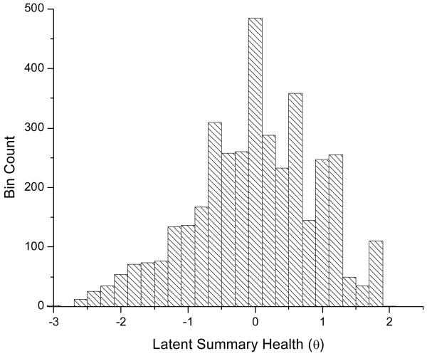
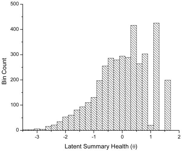
Our IRT analysis derived θ̂_is for all 3488 respondents under the convention that the population mean is 0 and standard deviation is 1. θ̂_i was estimated if at least 1 index was nonmissing. No one was missing all 5 indexes; 264 respondents had 1 or 2 missing indexes, and 17 were missing 3 or 4 index scores. The mean of fitted θ̂_is was –0.0014 (standard deviation, 0.93); the median was 0.03. Figure 1 shows a histogram of θ̂_is. The empirical distribution skews slightly with a longer tail toward negative θ (poorer health).

Figure 1.

Histogram of item response theory (IRT)-calculated latent summary health scores (θ) for 3844 individuals.

Low θ̂_is were associated with people who reported poor health in more ways than just through the index scores (e.g., there were 35 individuals with θ̂_i = –2.0 ± 0.05, approximately 2 standard deviations below the population mean). One example of these was a 47-year-old-woman who was living without a spouse in a rural area. Based on self report she is a former smoker with body mass index (BMI) of 39, has diabetes but does not use insulin, had been told by a doctor she had a gastrointestinal ulcer, and had no health insurance in the past 12 months. She rated her health as “poor.” Her EQ-5D score was 0.38, HUI2 was 0.25, HUI3 was 0.0, SF-6D was 0.46, and QWB-SA was 0.35, and her health had stopped her usual activities in all 30 of the past 30 days. Another of the 35 individuals was an 83-year-old-woman with BMI of 24 living with her spouse in a rural area. She rated her health as “poor” and reported cataract, arthritis, and chronic back pain from a herniated disk for which she currently takes medication^*. Her EQ-5D was 0.44, HUI2 was 0.14, HUI3 was –0.02, SF-6D was .51, and QWB-SA was 0.36. She too reported her health stopping usual activities in 30 of the past 30 days.

Individuals with θ̂_i = 0.0 ± 0.05, at the middle of the population, reported much better health. There were 371 individuals with θ̂_i in this range. Among these was a 47-year-old-man with BMI of 27, living in an urban area with his spouse. He self-rated his health as “fair,” and although a smoker, he reported only arthritis out of the 11 health conditions prompted in the interview. His HRQoL scores were as follows: EQ-5D = 0.80, HUI2 = 0.85, HUI3 = 0.85, SF-6D = 0.81, and QWB-SA = 0.66. In the past 30 days he said his health had stopped usual activities on none. A second example was a 56 year old woman with BMI of 33, who self-rated her health as “very good.” She reported none of the 11 health conditions, and no days in the past 30 where health stopped usual activities. Her index scores: EQ-5D = 0.83, HUI2 = 0.77, HUI3 = 0.84, SF-6D = 0.80, and QWB-SA = 0.61.

People with θ̂_i at or above 1.5 generally self-rated their health as either “very good” or “excellent,” tended to be younger, reported no or minor health conditions, lived in urban areas, and were scored at 1.0 on 2 or more of the HRQoL indexes.

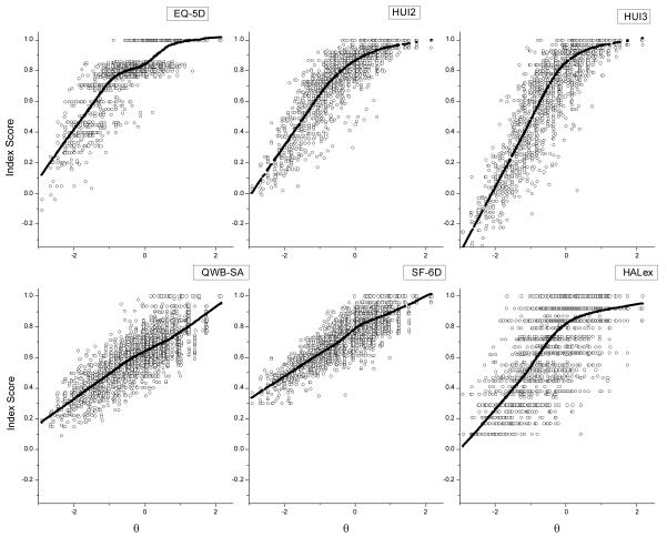
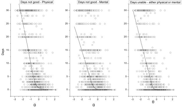
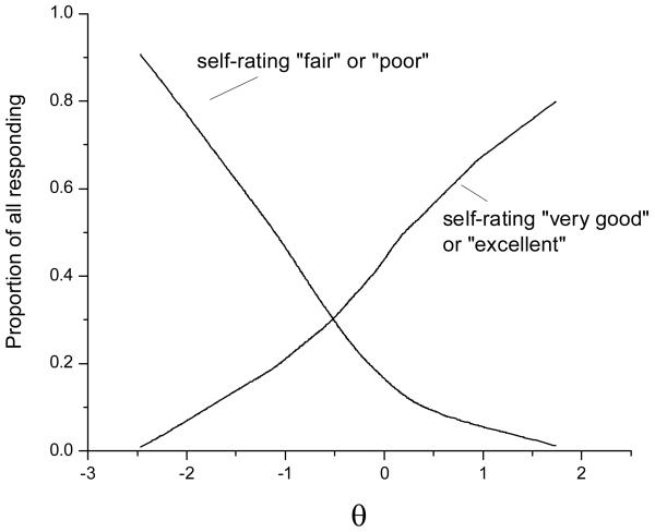
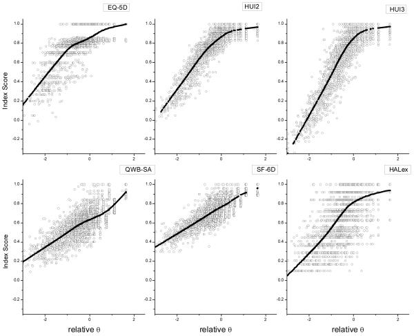
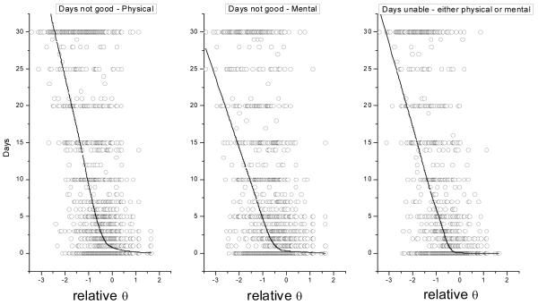
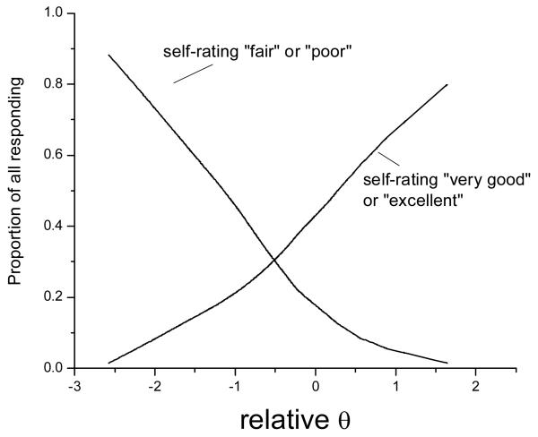
Figure 2 shows the 5 HRQoL indexes from which θ was estimated plotted versus θ. Also shown in Figure 2 is the HALex v. θ for each individual; the increased variance in scores on HALex conditioned on θ compared to the other panels is partly due to the fact that HALex was not one of the indexes used to estimate θ. The 3844 data points in each panel of this plot have been lightened and decreased in size to allow visual emphasis for the LOWESS curves fitted in each panel. Similar plots are shown for the CDC Healthy Days questions (Figure 3), and for moving average percentages of respondents self-rating their health as fair or poor, or very good or excellent, v. θ (Figure 4).

Figure 2.

The 6 panels plot index scores v. θ for the 5 main health-related quality-of-life (HRQoL) indexes and the Health Activities Limitations Index (HALex). Horizontal and vertical banding for the 3844 data points in each plot represents discrete attainable levels for the index or derived θs. The heavy lines are points fit using Minitab^®15.1 statistical software and the locally weighted scatterplot smoothing (LOWESS) option, a variant of kernel smoothing in the vertical dimension of scatterplots.[16] The LOWESS lines demonstrate nonlinearity of the relation between the index scales and θ.

Figure 3.

Scatterplots of “Healthy Days” questions v. θ. These questions ask respondents how many days out of the past 30 their physical health and mental health was “not good.” The third question (H-Days all) asks out of the past 30 days how many days did poor physical or mental health keep the respondent from doing usual activities such as self-care, work, or recreation. The heavy lines are LOWESS smoothed lines as in Figure 2. Each scatterplot displays 3844 data points (gray circles).

Figure 4.

Smoothed proportions of National Health Measurement Study (NHMS) respondents self-rating health as “fair” or “poor” and as “very good” or “excellent” as a function of θ. The proportions of responses in these categories were calculated for a window of 50 data points moving from θ=–2.5 through θ=2 for the 3844 observations. The resulting proportions were then Locally Weighted Scatterplot Smoothing (LOWESS)- smoothed as described for Figure 2 and the result shown here.

Fit of the IRT Model

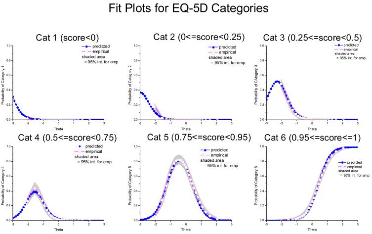
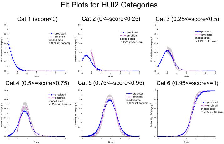
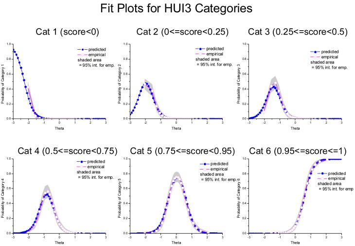
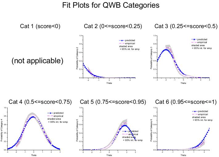
Inspection of fit plots for the 5 indexes (see Appendix 1at http://mdm/sagepub.com/supplemental) suggested an adequate fit—especially in the upper two-thirds of the θ continuum The software MODFIT (Version 1.1, 2001 © Stephen Stark, IRT Modeling Lab, University of Illinois at Urbana-Champaign, http://work.psych.uiuc.edu/irt/mdf_modfit.asp, accessed 1 July 09) was used to evaluate fit statistics and compute fit plots. Although adjusted chi-square statistics show poor fit where data are sparse at the lowest levels of health, fit was quite good in the upper two-thirds of the health continuum where the indexes are most different from one another.

Local dependence was evaluated by determining whether there were significant correlations among residuals after θ was removed from the original index scores. Table 3 displays correlations among LOWESS residuals (index score minus the LOWESS fit curve for each respondent) for the 5 primary HRQoL indexes and the HALex. These correlations tested whether θ summarizes all common information among the indexes or whether there is still common information in the residual variance conditioned on θ. The correlation between residuals from HUI2 and HUI3 was expected to be larger than correlations between these residuals and those associated with other indexes because HUI2 and HUI3 are not locally independent as previously noted. The other modest residual correlations, significant due to large sample size, are consistent with artifact caused by ceiling effects.

Table 3.

Pairwise Pearson correlations among the residuals around the LOWESS lines in Figure 2 for 3844 respondents.

	EQ-5D	HUI2	HUI3	QWB-SA	SF-6D
HUI2	–0.29*
HUI3	–0.38*	0.42***
QWB-SA	–0.15*	–0.08*	–0.10*
SF-6D	–0.11*	–0.17*	–0.22*	–0.16*
HALex	0.03	–0.04**	0.002	0.10*	0.14*

EQ-5D, EuroQoL EQ-5D, Health Utilities Index Mark 2; HUI3, Health Utilities Index Mark 3; QWB-SA, Quality of Well-Being Index Self-Administered Version; SF-6D, a utility-valued summary scale based on data from the SF –36v2 ™ ; HALex, Health Activities Limitation Index; LOWESS, locally weighted scatterplot smoothing.

^*P< 0.001

^**P < 0.05

^***P <0.001 (this correlation also reflects common variance in HUI2 and HUI3 due to the fact that they are two different calculations using the same set of answers to 40 questions).

Robustness of IRT Results for Alternative Categorization of Indexes

A number of auxiliary experiments to estimate θ̂_is showed the derived θ̂_is to be quite robust. Modestly revised category boundaries (moving the cutpoints up or down by .05) and estimation with other software programs produced results similar to our primary analyses. All the comparisons yielded θ̂_is that were highly correlated with the primary results (results not shown). IRT software usually will accommodate 4 to 10 categories for items in the graded response model. We believe 6 categories are necessary to differentiate indexes that score cases below 0.0 from those that do not, as well as to differentiate indexes that have many observations at the ceiling from indexes that have little or no ceiling effect. When we used 8 categories, placing cutpoints at 0, 0.25, 0.5, 0.6, 0.7, 0.8, and 0.9, these cutpoints emphasize the upper half of the utility scale where most cases reside - the resulting θ̂_is correlated at r = 0.97 with our 6-category θ̂_is. The mean absolute deviation between the 2 sets of θ̂_is is 0.19 across the 3844 respondents. Because of the gap in the EQ-5D score distribution between 1.0 and 0.86, due to the nature of the US valuation weights, placing more cutpoints at the top of the utility scale is not feasible. Because the 8-category θ̂_is did not produce different results in any essential way from the 6-category θ̂_is, we report the latter here as being most parsimonious.

To this point, we have reported θ̂_is based on a 6-category scheme fixed for all indexes. For HUI2, HUI3, and EQ-5D, all 6 categories were populated. For QWB-SA, 5 categories were populated. The SF-6D data used only 4 of these categories. As an alternative categorization scheme, such that each index was divided into 6 populated categories, we used a relative partition: we divided the range between each individual index’s minimum possible score for a living person and 1.0 into 6 equal-length categories. Thus, for HUI3, the range from –0.36 to 1.0 was divided into 6 equal-length categories, and for SF-6D, the range from +0.3 to 1.0 was divided into 6 equal-length categories. The resulting partitions were relative to each index’s own minimum and maximum scores so that no categories were artificially empty for any index. Each index had its own unique partition in this scheme. The resulting categorized variables were analyzed with SCORIGHT and the graded response model, again presuming HUI2 and HUI3 nonindependent. The correlation between the θ̂_is derived from the relative partitions and the θ̂_is derived from the original fixed partition was 0.94. Plots corresponding to those shown in Figures 1 to 4, but using the θ̂_is from the relative partitions were essentially the same as the original Figures 1-4 (see Appendix 2 at http://mdm/sagepub.com/supplemental).

DISCUSSION

Our primary objective was to describe how the 5 HRQoL indexes—EQ-5D, HUI2, HUI3, QWB-SA, and SF-6D—each relate to a common construct of underlying summary health and, in turn, to each other. Figure 2 is the main tool for comparison. It is important to realize the scale for θ is somewhat arbitrary and useful to imagine the graphs with monotonic rescaling of θ to compress or stretch the upper end of its scale. If the region between approximately 0 and +2 on the θ axis were compressed, the upper ends of the LOWESS curves for EQ-5D, HUI2, HUI3, and HALex would tend to straighten, and the LOWESS lines for QWB-SA and SF-6D would tend to curve upward in this region. But no monotone rescaling of θ will make the relationships between EQ-5D, HUI2, HUI3, or HALex linear with QWB-SA and SF-6D across the entire range of θ. The implication of this is that if one wishes to cover the full range of θ then no simple linear transformation exists for a crosswalk between any choice of index from the set {EQ-5D, HUI2, HUI3, HALex} and an index from {QWB-SA, SF-6D}. It does appear that a linear crosswalk between QWB-SA and SF-6D is feasible.

Figures 2 to 4 show that θ, which was estimated as an underlying summary construct for information common to EQ-5D, HUI2, HUI3, QWB-SA, and SF-6D, is also strongly associated with other HRQoL-related variables not used in estimating θ — HALex, the CDC Healthy Days questions, and self-rated health. Our results provide good empirical support for a unidimensional construct of summary health common to a variety of summary HRQoL measures.

Below approximately θ = –0.5 all 6 indexes appear to vary linearly with θ. In this region of summary health simple linear functions will transform one index score to another. The precision of these transformations will be low at the individual person level because the variance in index scores around the LOWESS lines is still relatively large given most values of θ. The relative slope of the LOWESS lines in each panel of Figure 2 below about θ = –0.5 is different for each of the indexes, with that for HUI3 being steepest and that for SF-6D being most shallow. Steeper slopes represent better precision to represent differences in θ, all other things being equal; in this respect, HUI3 appears to better represent the common information in the collection of indexes for individuals with θ̂_is substantially below the population mean.

None of the indexes is consistently best in the sense of having the steepest relative slope across the full range of θ as judged by the relative slopes in different regions of θ. The HUI3 has the steepest slope, indicating large changes in index scores to reflect changes in θ, but the HUI3 also shows decreasing slope as θ ranges above the population average (θ = 0). The QWB-SA and SF-6D both have little change in slope above or below θ=0, but their slopes are less steep overall than for the other indexes. Where HUI2, HUI3, and HALex show small changes in score for changes in θ above the population average, the QWB-SA and SF-6D show similar changes in score for θs above and below the population average.

The EQ-5D is anomalous, having in effect 2 ceilings. The first “ceiling” is around an EQ-5D score of 0.8, the first inflection in the LOWESS curve, and there is a large cluster of observations just below this point, ranging approximately between θ = –1.3 and θ = 0.75. The second and true ceiling is at EQ-5D score of 1.0 and is seen as a second inflection of the LOWESS curve. The gap is likely due to the EQ-5D descriptive system in which the top health state apparently covers a broad range of relatively mild differences in health [17].

With respect to the underlying summary health construct common to all, 4 of the 6 indexes show increasing compression of scores for health states above the mean of θ. Much of this compression may be due, as in the case of the EQ-5D, to their inability to differentiate among relatively good health states. But at least part of the compression may also reflect differences in the community’s valuation of relatively good health states among the different indexes. Where each of the 5 indexes, as well as the HALex, appear to have modest ability to differentiate states of health above the mean, the CDC Healthy Days questions have no ability to do so; they solely reflect varying degrees of quite poor health below θ = 0.

In the NHMS sample, we see no noticeable floor effects—that is, there is no compression of scores or flattening of the LOWESS lines for health states at the lowest end of the θ continuum, as if the index scale had encountered a lower bound and could not reflect even worse health states. In this community-living sample, health states that were scored at the lowest possible score were in fact reported by some individuals for each of the indexes. Very ill, institutionalized individuals can be qualitatively more sick than respondents in this sample, but they can not receive lower scores on any index than the scores observed here. Nonetheless, it is the case that relatively few very ill respondents were likely to respond in a telephone survey of community-living individuals. Therefore we may not have observed the full spectrum of health states that would be found in very ill people and so our ability to observe floor effects mentioned in other studies (e.g., Brazier and Roberts [18], Blanchard, Feeny Mahon and others [19]), was likely attenuated. Because nonresponse in a telephone survey also can be due to people in good health being too busy to participate, nonresponders can also be found at the other end of the health continuum. A limitation of our study is that we cannot assess the impact of nonresponse bias in NHMS on our overall results.

Each index relates strongly to θ, but each also has a large variance conditional on θ (i.e., a wide vertical spread in index scores at any given level of θ). Because θ is a composite of the indexes, this variance conditioned on θ is unique to each index and may in part represent meaningful variation not summarized in the other indexes and in part statistical noise. The correlations of residuals in Table 3 may be statistically significant primarily because of the large sample size. We suspect the larger correlations are an artifact of ceiling effects (correlation is induced because errors can go in only one direction, away from the ceiling) rather than a reflection of meaningful variation not contained in θ; the lower ranges of θ scatterplots (not shown) show the residuals are essentially uncorrelated when θ is below 0. Gaining an understanding of the content and classification value of the unique variance for each index is important to an overall understanding of the total contribution of each index, but beyond our current analysis, which focuses on the common variation in the indexes.

Is there a best index to measure the common summary health construct represented by θ? First, although we’ve put it at disadvantage by not including it as a basis for estimating θ, the HALex clearly is a less precise measure of θ. Given one must choose from the remaining 5 indexes, we believe the answer to the question is no. There are pros and cons to each.

For measuring health toward the lower ranges of θ, all 5 indexes have essentially a linear relationship with θ and about the same variance conditioned on θ. The steepness of the HUI3’s relation with θ favors it being most responsive to differences among states of poor health. For differentiating among very good health states, the QWB-SA and SF-6D may offer an advantage over the other 3 indexes because they have slightly steeper slopes than the others and small or no discernible ceiling effect. Clearly, the EQ-5D leaves much to be desired for measuring health from about 1 standard deviation below the population mean upward as its descriptive system (especially with the US scoring weights) leads to the curious double ceiling effect.

Choice of index may also be influenced by issues of questionnaire length and whether the investigator wants to avoid a proprietary instrument. QWB-SA is a longer questionnaire, but gives detailed information about symptoms as it is mostly symptom-driven. SF-6D is based on a proprietary questionnaire, the SF-36v2™, and is mostly driven by self-reported functioning and functional capability.

For measuring health in lower ranges of θ, the dispute is not only which index has the better psychometrics, but which is the “real” utility scale. All 6 appear to be nearly linear transformations of one another for health states below the midrange of θ in our survey data. This begs the question, “Which is the correct scale to use?” This is an important question for cost-utility analyses meant to inform public policy. Its answer seems to hinge largely on whether states may be scaled worse than dead or not, as having scores less than 0.0 substantially stretches an index’s scale relative to indexes that stop at 0.0. There is enough unique variance associated with each index to dim prospects for translating scores for individuals from one index to another despite the magnitude of the common variance. However, for measuring health of groups of individuals who are expected to have average health below the population mean, the linearity of the scales with θ holds good promise for simple crosswalks among group means as we would expect more or less constant offsets between means measured on the different scales. We speculate that the precision of crosswalks among group means may be quite good. These observations extend to the CDC Healthy Days questions as well—the relation between mean healthy days and θ is linear, albeit with high conditional variance, for each question when θ is less than zero. For health states represented by θ greater than 0 there is no relation between the healthy days questions and θ.

Our data are limited for assessing the broad range of health states in the seriously ill, so we must qualify our discussion here, recognizing that we are basing our observations on population data.

CONCLUSION

A single concept we denote “latent summary health” subsumes the HRQoL measures used in this analysis. There is good reason to expect that simple, albeit low-precision, linear crosswalks can be derived among the EQ-5D, HUI2, HUI3, QWB-SA, and SF-6D for health states below the population mean of latent summary health, as all of these indexes appear to be linearly related in this range. However, increasing compression of scores with better health for EQ-5D, HUI2, and HUI3 means that crosswalk equations for these must have 2 linear parts with differing slopes. The compression is such that variance unique to each index is likely to moot the usefulness of a crosswalk for health states above the mean of a community-living sample of adults.

For less healthy individuals, crosswalks among the indexes may be useful at the level of group mean HRQoL and may be accomplished by simple linear functions from one index to another. Policy-directed cost-effectiveness analyses often include just such group comparisons. For these, the issue is not which index is better psychometrically but which utility scale correctly represents the values which the analysis wishes to encompass. This choice is an issue our analyses highlight, but cannot settle.

Figure A2–1.

Histogram of IRT-calculated latent summary health scores (Relative θ) for 3844 individuals.

Figure A2–2.

The six panels plot index scores versus Relative θ for the 5 main HRQoL indexes and the HALex. The heavy lines are points fit using Minitab®15.1 statistical software and the locally weighted scatterplot smoother (LOWESS) option.

Figure A2–3.

Scatterplots of “healthy days” questions versus Relative θ. These questions ask respondents how many days out of the past 30 their physical health, mental health was “not good.” The third question (H-Days all) asks out of the past 30 days how many days did poor physical or mental health keep the respondent from doing usual activities such as self-care, work, or recreation. The heavy lines are LOWESS smoothed lines as in Figure 2. Each scatterplot displays 3844 data points (gray circles).

Figure A2–4.

Smoothed proportions of NHMS respondents self-rating health as “fair” or “poor” and as “very good” or “excellent” as a function of Relative θ. The proportions of responses in these categories were calculated for window of 50 data points moving from θ=-2.5 through θ=2 for the 3844 observations. The resulting proportions were then LOWESS smoothed as described for Fig. A2–2 and the result shown here.

on-line Appendix 1

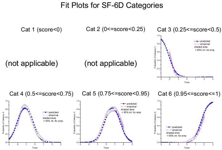
This appendix presents the parameters and fit plots for the IRT model reported in the paper.

Data for each of the 5 HRQoL indexes were categorized into 6 score ranges. The categories and Ns for each index are shown in table A-1:

Table A-1.

Sample sizes for each category for each index

Index	Cat. 1 (score < 0.0)	Cat. 2 (0.0≤score<0.25)	Cat. 3 (0.0≤score<0.25)	Cat. 4 (0.0≤score<0.25)	Cat. 5 (0.0≤score<0.25)	Cat. 6 (0.0≤score<0.25)
EQ-5D	4	44	198	307	1866	1393
HUI2	1	89	197	523	1615	1133
HUI3	88	184	276	574	1331	1114
QWB-SA	Not applicable*	64	677	2279	734	90
SF-6D	Not applicable*	Not applicable*	191	1368	1872	308

Row sums are not equal due to missing scores, which could not be categorized.

^*The theoretical definition for this index does not allow scores of living persons to fall in the indicated range.

Table A-2 show the IRT parameters derived for each of the indexes. For each index there is a slope parameter and cutoff parameters corresponding to the categories. The expected frequencies of responses are computed based on these parameters and the standard graded response IRT model.

Table A-2.

IRT model parameters derived for each index.

Index	a (slope)	b1	b2	b3	b4	b5
EQ-5D	1.6005	–3.2901	–2.71744	–1.86808	–1.25956	0.424558
HUI2	1.7687	–2.803	–2.3236	–1.68263	–0.84981	0.582458
HUI3	2.0798	–2.2766	–1.68684	–1.16332	–0.50461	0.597744
QWB-SA	1.1255	–2.8425	–1.15416	1.066252	2.469353	Not applicable*
SF-6D	1.5033	–2.0605	–0.20721	1.625451	Not applicable*	Not applicable*

the parameters, bi (i=1..5) are cutoff values for the categories.

^*This categories not used.

Fit plots are shown in Figures A-1 through A-5 for each category for each index. The predicted response curves were computed using the derived index parameters. The empirical curves and intervals are based on the observed data in each category conditioned on theta. These curves were fit using the program MODFIT (Available at University of Illinois IRT Modeling Lab web site, http://io.psych.uiuc.edu/irt/downloads.asp, accessed Jan. 28, 2009).

The shaded areas in each plot are 95% intervals fit for the empirical data for a grid of theta values and then connected smoothly.

On-line Appendix 2

This appendix presents 4 figures paralleling those in the main text. However these figures use latent summary health measured with Relative θ as described in the main text.

These θ̂_is were derived based on six-category partitions of the 5 HRQoL indexes, EQ-5D, HUI2, HUI3, QWB-SA, and SF-6D where each partition was constructed by placing 5 cutpoints, equally spaced between the minimum and maximum scores attainable by living persons, separately for each index.

As seen in Fig A2–1, Relative θ̂_is are somewhat more skewed than the θ̂_is in the main paper, and the distribution shows two spikes in estimated θ̂_is.

REFERENCES

- 1.Houle C, Berthelot J-M. A Head-to-Head Comparison of the Health Utilities Index Mark 3 and the EQ-5D for the Population Living in Private Households in Canada. Quality of Life Newsletter. 2000;24:5–6. MAPI Institute. [Google Scholar]
- 2.Kaplan RM, Groessl EJ, Sengupta N, et al. Comparison of measured utility scores and imputed scores from the SF-36 in patients with rheumatoid arthritis. Med Care. 2005;43:79–87. [PubMed] [Google Scholar]
- 3.Luo N, Chew LH, Fong KY, et al. A comparison of the EuroQol-5D and the Health Utilities Index mark 3 in patients with rheumatic disease. J Rheumatol. 2003;30:2268–74. [PubMed] [Google Scholar]
- 4.Luo N, Johnson JA, Shaw JW, et al. Self-Reported Health Status of the General Adult US Population as Assessed by the EQ-5D and Health Utilities Index. Med Care. 2005;43:1078–86. doi: 10.1097/01.mlr.0000182493.57090.c1. [DOI] [PubMed] [Google Scholar]
- 5.Pickard AS, Johnson JA, Feeny DH. Responsiveness of generic health-related quality of life measures in stroke. Qual Life Res. 2005;14:207–19. doi: 10.1007/s11136-004-3928-3. [DOI] [PubMed] [Google Scholar]
- 6.Davison SN, Jhangri GS, Feeny DH. Comparing the Health Utilities Index Mark 3 (HUI3) with the Short Form-36 Preference-Based SF-6D in Chronic Kidney Disease. Value Health. 2009;12:340–5. doi: 10.1111/j.1524-4733.2008.00433.x. [DOI] [PubMed] [Google Scholar]
- 7.Fryback DG, Dunham NC, Palta M, et al. US Norms for Six Generic Health-Related Quality-of-Life Indexes From the National Health Measurement Study. Med Care. 2007;45:1162–70. doi: 10.1097/MLR.0b013e31814848f1. [DOI] [PMC free article] [PubMed] [Google Scholar]
- 8.Shaw JW, Johnson JA, Coons SJ. US valuation of the EQ-5D health states: Development and testing of the D1 valuation model. Med Care. 2005;43:203–20. doi: 10.1097/00005650-200503000-00003. [DOI] [PubMed] [Google Scholar]
- 9.Erickson P. Evaluation of a population-based measure of quality of life: the Health and Activity Limitation Index (HALex) Qual Life Res. 1998;7:101–14. doi: 10.1023/a:1008897107977. [DOI] [PubMed] [Google Scholar]
- 10.Moriarty DG, Kobau R, Zack MM, et al. Tracking Healthy Days: a window on the health of older adults. Prev Chronic Dis. 2005;2:A16. [PMC free article] [PubMed] [Google Scholar]
- 11.Nunnally JC, Bernstein IH. Psychometric theory. 3rd ed. McGraw- Hill; New York: 1994. [Google Scholar]
- 12.Baker FB, Kim S-H. Item Response Theory, Parameter Estimation Techniques. Marcel Dekker, Inc.; New York: 2004. [Google Scholar]
- 13.Linting M, Meulman JJ, Groenen PJF, et al. Nonlinear principal component analysis: Introduction and application. Psychological Methods. 2007;3:336–58. doi: 10.1037/1082-989X.12.3.336. [DOI] [PubMed] [Google Scholar]
- 14.Wang X, Bradlow ET, Wainer H. A general Bayesian model for testlets: theory and applications. Applied Psychological Measurement. 2002;26:109–28. [Google Scholar]
- 15.Wang X, Bradlow ET, Wainer H. User’s Guide for SCORIGHT (Version 3.0): A Computer Program for Scoring Tests Built of Testlets Including a Module for Covariate Analysis. Educational Testing Service; Princeton New Jersey: 2005. [Google Scholar]
- 16.Cleveland WS. Robust locally weighted regression and smoothing scatterplots. Journal of the American Statistical Association. 1979;74:829–36. [Google Scholar]
- 17.Insinga R, Fryback D. Understanding differences between self-ratings and population ratings for health in the EuroQOL. Qual Life Res. 2003;12:611–9. doi: 10.1023/a:1025170308141. [DOI] [PubMed] [Google Scholar]
- 18.Brazier JE, Roberts J. The estimation of a preference-based measure of health from the SF-12. Med Care. 2004;42:851–9. doi: 10.1097/01.mlr.0000135827.18610.0d. [DOI] [PubMed] [Google Scholar]
- 19.Blanchard C, Feeny D, Mahon J, et al. Is the Health Utilities Index valid in total hip arthroplasty patients? Qual Life Res. 2004;13:339–48. doi: 10.1023/B:QURE.0000018479.52075.bf. [DOI] [PubMed] [Google Scholar]