Disentangling the Effect of Local and Global Spatial Variation on a Mosquito-Borne Infection in a Neotropical Heterogeneous Environment

Abstract

Mosquito-borne pathogen transmission exhibits spatial-temporal variability caused by ecological interactions acting at different scales. We used local spatial statistics and geographically weighted regression (GWR) to determine the spatial pattern of malaria incidence and persistence in northeastern Venezuela. Seven to 11 hot spots of malaria transmission were detected by using local spatial statistics, although disease persistence was explained only for four of those hot spots. The GWR models greatly improved predictions of malaria risk compared with ordinary least squares (OLS) regression models. Malaria incidence was largely explained by the proximity to and number of Anopheles aquasalis habitats nearby (1–3 km), and low-elevation terrains. Disease persistence was associated with greater human population density, lower elevations, and proximity to aquatic habitats. However, there was significant local spatial variation in the relationship between malaria and environmental variables. Spatial modeling improves the understanding of the causal factors operating at several scales in the transmission of malaria.

Introduction

Human malaria, one of the most serious parasitic diseases of tropical ecosystems, is caused by parasites of the genus Plasmodium (Apicomplexa: Plasmodidae) and transmitted among human hosts by the bites of infected female Anopheles mosquitoes (Diptera: Culicidae). In 2006, malaria was responsible for 247 million clinical cases among 3.3 billion people at risk, causing nearly a million deaths.¹ The dependence of malaria transmission on its spatial and ecological context has long been recognized; hence, the need to study this disease within its explicit spatial context.^2–5 Transmission of mosquito-borne pathogens can be highly heterogeneous caused by a complex set of interactions among parasites, vectors, and hosts occurring at specific locations (both natural and anthropogenic landscapes), and at specific times.^6–8 Efficient control of this disease and prediction of its emergence or spread to new geographic regions require an understanding of the effect of spatial heterogeneity on malaria transmission dynamics.^5,6 Ecoepidemiologic patterns can result from various processes (extrinsic and intrinsic) simultaneously acting at different scales.⁹ Thus, disentangling the spatial scales of these processes should be an aim in studies of the landscape epidemiology of malaria.

Spatial heterogeneity can be caused by spatial-temporal structuring of the physical environment, which induces similar spatial aggregation of individuals and populations in the landscape by creating large-scale trends (e.g., > 100 km).⁹ As an example, malaria is uncommon in high-elevation areas because the parasite, as well as the mosquito, requires warm temperatures (e.g., > 21°C for Plasmodium), high humidity (> 80% for mosquito adults), and suitable wetlands or aquatic habitats for mosquito pre-adults to complete their life cycles and survive. Hence, the landscape directly influences the spatial pattern of transmission by creating nonrandom distributions of pathogens and vectors, and acts like a selective filter on the establishment of local mosquito–parasite and human interactions.⁹ At intermediate (e.g., < 100 km) and local scales (e.g., 100 m to 5 km), the risk for malaria is mainly determined by human and mosquito behavior and ecology, especially the distribution of blood-meal hosts and water. In this case, underlying environmental conditions do not generate the spatial pattern of infection; rather the observed pattern is the result of intrinsic population-related processes, which increase local interactions at the expense of global connectedness. The degree of spatial dependency generated either by exogenous or endogenous processes, and the relevance of differentiating both spatial scales has been well recognized in ecology^10,11 and very recently in some infectious disease dynamics.^8,9,12 Paradoxically, though the results of malaria modeling are more often spatially presented (e.g., as a geographic information system [GIS]-derived map of the predicted disease distribution at global and/or local scale), spatial information is not usually accounted for in the model itself, except in some recent attempts.^13,14 However, predicting mosquito-borne pathogen transmission using global nonspatial predictive models is difficult to assess because of non-stationarity (the variation in modeled relationships over space), which is likely to be a very common property in ecological systems.¹⁰

We sought to determine and predict the spatial variation of Plasmodium vivax malaria infection in an epidemic-prone Neotropical area, in northeastern Venezuela. We emphasized the relevance of using local spatial analytical approaches such as local cluster detection (e.g., local Getis statistic)¹⁵ and geographically weighted regression (spatially explicit model)¹⁶ to identify and understand the major determinants of malaria risk and disease differences across space. Specifically, we described the spatial heterogeneity of malaria, identified the spatial extent or scale of the disease process, and showed that the relationship between malaria and the environmental factors varies across space.

Material and Methods

Study area.

The study area (332.5 km²) is located in the southern lowland area of Sucre State (Cajigal Municipality), in northeastern Venezuela (10°34′N, 62°49′W). This rural zone bordering the Caribbean Sea corresponds to the coastal ecoregion,¹⁷ where malaria is endemic and P. vivax is transmitted by Anopheles (Nyssorhynchus) aquasalis Curry.¹⁸ Specifically, more than 90% of the malaria cases of Sucre State in recent years have occurred in this municipality.¹⁹ The area has an estimated population of 24,345 inhabitants and 3,587 houses (2001 Venezuelan census) distributed in 29 villages interconnected by primary (paved) and secondary (dirt) roads, with a mountain range in the northern sector reaching up to 600 m altitude. Vegetation is composed of sparse patches of deciduous forests, cleared lands for small crops and coconut groves, large zones of herbaceous and woody swamps, and large, relatively undisturbed coastal mangroves.²⁰ Annual mean temperature is 27–28°C and total annual rainfall is 1,200–1,700 mm, with a rainy season from May to November and a dry season from December to April.

Epidemiologic data.

Village-level case data of P. vivax malaria from 2001 to 2007 (positive blood smears) were obtained from the Malaria Control Program database, Venezuelan Ministry of Health, where symptomatic cases are detected by passive and active surveillance. The Division of Environmental Health compiles all notifications of malaria consultations on a weekly basis, and cases are reported using the patient's address. We analyzed data from 22 of the 29 villages of the municipality because of a lack of accuracy about their population data of seven villages. We avoided the bias arising from P. vivax relapses²¹ by considering only one positive blood smear per individual per year (single malaria episode). No personal identifiers were used in this study, which was ethically approved by the Venezuelan Council for Scientific Research. To calculate the malaria incidence rates per 1,000 inhabitants by locality (annual parasite incidence [API] = no. of new cases × 1,000/population at risk per year), we assumed that the entire population of the villages was exposed to the risk of contracting malaria; i.e., each person contributed exactly 1 person-year of exposure. The 95% confidence limits for the incidence data were computed by assuming an underlying Poisson distribution.²² The P. vivax infection persistence (IP) by locality by year was calculated as the maximum number of consecutive weeks a village had malaria cases.³ ArcGIS 9.1 (ESRI Corporation, Redlands, CA) software was used to display the distribution of malaria incidence (API) per village by year.

Environmental predictors of malaria risk.

Specific landscape features, socioepidemiologic attributes, and ecologic variables were used to explain and predict the spatial variation of malaria incidence and persistence in the study area. These variables were terrain elevation, terrain slope, number of inhabitants per village, distance to the main road, number of immature Anopheles aquasalis habitats within a circular buffer zone of 1 km centered on each village (here considered as the effective flight range of the mosquitoes), and distances to the nearest immature An. aquasalis habitat, or to the closest wetland or mangrove from each locality. In a previous study in the western part of this malaria focus, most of these variables were risk factors for P. vivax transmission.³ Landscape variables were derived from a GIS or digitized from topographic maps (1:100.000; Ministry of Environment, 1999). Elevation and slope were calculated as averages for each community based on elevation maps with contour lines every 30 m.

From 2002 to 2005, we surveyed 87 aquatic habitats, which generated 55 sampling points (positive for An. aquasalis) that were incorporated into the GIS. Mosquito samples were taken with a standard dipper, and anopheline occurrence in aquatic habitats was confirmed (from 30 such samples) by visiting the area periodically (dry and rainy season per year) throughout that period. Our previous studies had found that this mosquito species was the most common, abundant, and widely distributed species in this region, showing its largest abundance in the mangrove swamps but also associated with herbaceous swamps (brackish and freshwater) and small freshwater bodies such as ponds.^20,23

Data analysis.

Hot spot detection.

The nonspatial dependency in the malaria distribution pattern would imply that an event of infection is equally likely to occur at any location within the study area, regardless of the locations of other events (i.e., a spatially constant risk). Consequently, the observed disease patterns would represent the normal variation in malaria incidence given the at-risk population distribution. To test that hypothesis, we used two local measures of spatial association, the Kulldorff scan statistic²⁴ and the local Getis statistic, G_i*(d).¹⁵

The Kulldorff scan statistics allowed us to identify significant excesses cases (e.g., the most likely cluster) of P. vivax incidence in space and time. The scan statistic uses a circular (space) or cylindrical (space-time) scanning window that moves systematically across space (study area) and/or time. The scanning window is centered on each sample at a particular time and expanded to include neighboring locations and time intervals until it reaches a maximum size (e.g., never including > 50% of the population-at-risk size for the study period). The null hypothesis is evaluated with a maximum likelihood ratio test (by assuming a Poisson distribution). The scan statistic is the maximum likelihood ratio over all possible window sizes. A P value provides the probability for the most likely cluster and is obtained through multinomial Monte Carlo randomizations.

The local Getis statistic, G_i*(d), identified significant local clustering of high positive (hot spots) or low negative (cold spots) values of malaria cases (e.g., weighted malaria cases standardized by the population at risk in each village) surrounding a particular village within a radius (circular window) of specified distance d from that location. The distance d defined the neighborhood search for a particular village, with nearby locations being expected to have similar values. The value obtained was compared (by using the Monte Carlo randomization procedure) with the statistic's expected value to indicate if the degree of clustering of malaria cases in the vicinity of a particular village was greater or less than expected by chance. To correct for multiple comparisons when using Gi*(d), significance levels were adjusted according to Getis and Ord's criteria.²⁵ We calculated Gi*(d) at different scales (5 distance categories) by using various window sizes (1 to 5 km, 1 km each) for each year. The maximum Gi*(d) distance corresponded to the scale at which Gi*(d) maximum value was found; i.e., the scale of the spatial dependence of the process under study. In addition, we used this analysis with yearly IP data to explore the spatial dynamics of malaria spread in this region. The analyses of Gi*(d) and Kulldorff scan statistics were carried out using the ClusterSeer software (TerraSeer, Ann Arbor, MI).

Local spatial and global nonspatial regression modeling.

The use of ordinary least squares (OLS) regression modeling has been by far the most common analytical approach to explain and predict variation in infectious diseases. The OLS regression assumes, however, that the data are normally distributed, the regression coefficients are “global” and apply equally to the entire study area, and residuals are spatially random, which is difficult to achieve given the spatial heterogeneity of the study area. When the data are spatially structured, OLS scores can be biased and their significance inflated.¹¹ A diagnostic statistic indicating problems in OLS regression with spatial data is the degree of spatial non-randomness of residuals; however, a common approach is to filter out or to treat the local spatial information as “noise.”¹⁰ Recently, spatial regression has been used,^10,16,26 yet these methods assume spatially stationary correlation structures that apply equally across the data set.

Geographically weighted regression (GWR) has been developed as an extension of traditional regression to incorporate, detect, and account for spatial non-stationarity in variable relationships in the model.¹⁶ This spatially localized model assumes that relationships between regression variables may vary over space; consequently, it generates a set of local linear regression models rather than a global model, with estimates for every sample in space. A moving window approach allows the weights of each spatial unit to vary as a function of the spatial relationship between them. Namely, a local estimation of model parameters is derived by using a subsample of data from nearby observations, which are weighted by using a decreasing function of distance. In this way, the impacts of neighboring samples are stronger than those farther away. A threshold, called the kernel bandwidth, is specified to indicate the distance beyond which neighbors no longer have influence on local estimates. The selection of the optimal bandwidth in the weighting function is reached by minimizing the corrected Akaike information criterion, AIC_c.¹⁶ A geographic surface of models is derived with associated goodness-of-fit statistics and localized parameter estimates such as R-square, standard error, and t values. These maps highlight possible data relationships, aid finding exceptions or local hot spots, and provide information on the nature of the processes under study. We used the GWR coefficient values to explore the spatial variability of relationships between malaria incidence or persistence and the selected geographic, environmental, and human predictors. To reach a more symmetric distribution, we log transformed the API and the IP data. We examined the significance of the spatial variability of local parameter estimates (spatial non-stationarity) after fitting the GWR model to all data by conducting a Monte Carlo test. In addition, we tested for spatial autocorrelation in the GWR residuals with the help of the Moran's I. For the purpose of comparison, OLS models were also derived and compared with the GWR prediction surface using the AIC_c and the global R². The GWR and OLS were conducted using the GWR software (version 3.0, Newcastle University, England, UK).¹⁶ Finally, we collapsed the 7 years and 22 observations into 154 data points to validate the OLS and GWR models with a greater sample size in a time-series approach. The malaria incidence and malaria persistence were modeled as a function of fixed and random (clustering) effects by using generalized linear mixed-effects models (GLMMs). The fixed effects quantified the overall effect (across all years) of the selected geographic, environmental, and human variables used in the OLS and GWR models, whereas the random effect quantified the variation of the temporal blocks (years) of the fixed-effect parameters.²⁷ We selected Poisson distribution models with logarithmic link functions and the estimation of parameters was based on penalized quasi-likelihood (PQL). We used the glmmPQL function available in the library MASS of the R statistical package²⁸ for fitting the GLMMs.

Results

Spatial clustering of malaria.

The total number of cases of malaria in the area during the study period was 8,360, with overall malaria incidence rates (cases per 1,000 person-year) ranging from 10 to 44 during 2001–2007 (Table 1). The highest value corresponded to the malaria epidemic of 2002, and over the 7-year period, the relative risk (RR) for P. vivax infections differed dramatically across the study site (Table 1).

Table 1.

Villages with the highest and lowest annual parasite incidence (API: cases × 1,000/year-person) during 2001–2007 in northeastern Venezuela^*

Year	API (95% CI)	Village with highest API	Village with lowest API	Relative risk (highest/lowest) (95% CI)
2001	45 (33–60)	174.3	2.5	69.7 (55–88)
2002	164 (140–192)	545.5	65.1	8.4 (4–16)
2003	44 (32–59)	154.8	2.9	53.4 (40–70)
2004	32 (22–45)	131.0	10.9	12.0 (6–21)
2005	29 (19–42)	100.0	4.7	21.3 (13–32)
2006	19 (11–30)	60.7	3.0	20.2 (12–31)
2007	10 (5–18)	35.7	1.0	35.7 (25–50)

^*CI = confidence interval.

Maps of malaria incidence for the whole region (Figure 1) show that most of the cases were spatially located toward the central and eastern area of the municipality where local clustering of P. vivax cases were detected with the scan statistic in every year (epidemic and nonepidemic years) around 7–11 villages (Figure 1A and B). Average malaria incidence within the cluster area was 1.9–2.7 times larger than malaria outside the cluster, indicating an increased risk of malaria for persons residing in those villages compared with those residing in the western or northern side of the municipality (Table 2).

Figure 1.

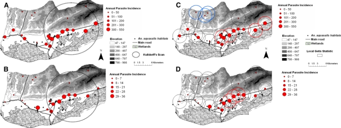
Annual parasite incidence (API: cases × 1,000/year-person) per village during 2002 (A, C) and 2007 (B, D) in Cajigal Municipality, northeastern Venezuela. Encircled areas in (A) and (B) denote significant clusters of diseases as detected by the Kulldorff scan statistic (P < 0.001). Encircled localities in (C) and (D) show the result of Gi*(d) analyses at a distance of 1 km, with significant (Gi*[d] > 2.79, P < 0.05) clusters of malaria infection in bold solid lines (hot spots, C, D) and broken lines (cold spots, C). Note the scale difference between API 2002 (A, C) and API 2007 (B, D). This figure appears in color at www.ajtmh.org.

Table 2.

Kulldorff's scan statistic results for the first most likely cluster of malaria incidence (API) in northeastern Venezuela

Year (no. of localities inside the cluster)*	Expected average disease frequency API (×1,000)	Observed average disease frequency† API (×1,000)	Relative risk†	Log-likelihood ratio
2001 (7)	44.3	118.5	2.7	65.5‡
2002 (11)	159.8	315.5	1.9	773.1‡
2003 (7)	43.7	111.4	2.5	194.1‡
2004 (10)	31.1	63.1	2.0	167.9‡
2005 (10)	31.1	58.8	1.9	175.2‡
2006 (10)	18.4	38.1	2.1	133.6‡
2007 (10)	9.4	19.3	2.0	64.7‡

^*Maximum spatial population radius analyzed (50% of total population).

^†Observed incidence in cluster/expected incidence outside the cluster.

^‡P < 0.01 (P values based on 999 simulations under the constant risk hypothesis).

A similar clustering pattern of high malaria incidence was observed with the local Getis statistic (Gi*[d] > 2.79, P < 0.05) at distances from 1 (Figure 1C and D) to 5 km (not all maps shown) around 3 to 10 central and eastern villages during all the analyzed years. During 2002, 3 cold spots (Gi*[d] < −2.79, P < 0.05) were detected with the local Getis statistic in the northwestern side of the region (Figure 1C). When space-time clustering was examined, the first 13 weeks of 2002 corresponding to the dry season met the Kulldorff scan criteria for a significant epidemic period when compared with records of weekly infection from other years (RR = 5.37, log-likelihood ratio = 2634.7, P < 0.001). Interestingly, malaria cases clustered in time around the same villages selected as hot spots in the spatial clustering (maps not shown).

There was a significant and positive correlation between malaria incidence and persistence (maximum consecutive weeks with malaria) by village (r_s = 0.89, N = 203, P < 0.01). The spatial analysis (local Getis statistic) of malaria persistence revealed significant clusters of 1 km (Gi*[d] > 2.79, P < 0.05) around four villages that were previously classified as hot spots and located in the central and eastern part of the region (maps not shown). These hot spots displayed up to 1 year of sustained malaria incidence.

Predicting malaria incidence.

Local spatial GWR models explained a larger portion of the variance (47–86%) than OLS regressions (18–57%) for each year of the study (Table 3). Although AIC_c values for GWR models did not decrease, as is usually expected with improved model fitting, it is also true that with more parameters AIC_c is penalized with increased values because of model overfitting. Local GWR's R² values per village were mapped to show the variation in the accuracy with which the model explained the variation in malaria incidence across the study area in 2002 and 2007; years with contrasting overall incidence (Figure 2). The maps indicate that local R² statistics were high for all the villages and studied periods, explaining from 61% to 98% of the variation in malaria incidence per village.

Table 3.

Model validation and main results of the ordinary least squares (OLS) regression and geographically weighted regression (GWR) models of malaria incidence (API) in northeastern Venezuela

Model (year)	AICc	R2	ANOVA
	OLS† | GWR†	OLS | GWR	F-value
2001	59.87 | 70.311	0.18 | 0.47	3.72*
2002	66.77 | 71.613	0.37 | 0.53	3.89*
2003	60.47 | 62.913	0.28 | 0.51	4.28*
2004	51.017 | 56.7913	0.33 | 0.47	2.94
2005	54.67 | 64.011	0.16 | 0.49	3.85*
2006	43.97 | 43.513	0.57 | 0.74	5.70*
2007	46.97 | 72.58	0.41 | 0.86	9.29**

Analysis of variance (ANOVA) tests the null hypothesis that the GWR model represents no improvement over the global OLS model. A Monte Carlo test compares the difference in the residual sums of squares of the OLS model with the residual sum of squares of the GWR model. R² represents the adjusted coefficient of determination, and AIC_c is the corrected Akaike information criteria. Model variables were population density, terrain elevation, terrain slope, number of aquatic habitats, distance to the nearest breeding site, and distance to the main road.

^*P < 0.05; ** P < 0.01.

^†DF of OLS and GWR residuals, respectively.

Figure 2.

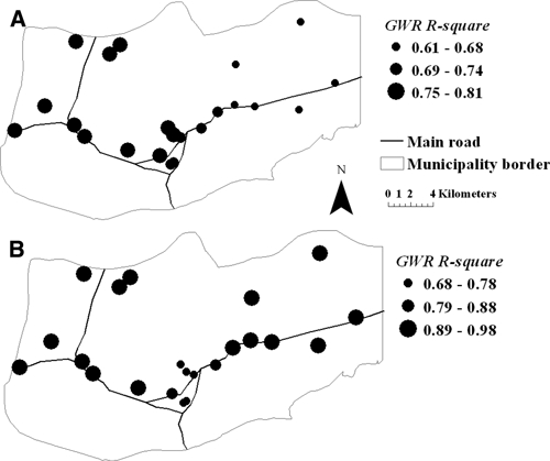
Spatial variation of local R² values or percentage of malaria incidence explained by each local GWR model during (A) 2002 and (B) 2007 in northeastern Venezuela.

Ordinary least squares regression models for each of the years of the study revealed that malaria incidence was positively associated with the number of An. aquasalis aquatic habitats that were located up to 1 km from villages (e.g., OLS model [2007]: β estimate ± SE [0.07 ± 0.03], t = 2.50, P < 0.05). Other variables included in the model did not show significant relationships with the variation of malaria incidence in the study area, and OLS model residuals exhibited significant spatial autocorrelation at the third lag (e.g., 2002: Moran's I = 0.39, Z-score = 2.11, P < 0.05; 2007: Moran's I = 0.33, Z-score = 2.11, P < 0.05). A more complex pattern with finer spatial variability in terms of the significance of the relationships between the explanatory variables and malaria incidence was depicted by the local GWR models. Although GWR general results supported those observed in the global nonspatial (OLS) regression model that linked malaria incidence with the number of mosquito aquatic habitats within a 1 km radius of each village, this variable was not significant everywhere, indicating the non-stationarity of the relationship of this ecological factor with malaria (Figure 3A). The number of An. aquasalis pre-adult habitats was a predictive variable (t values > 1.71, P < 0.05) across all regions except in some localities on the eastern side of the municipality. Certainly, malaria incidence in four eastern villages was not significantly associated with the number of aquatic habitats but with two other variables acting at different spatial scales, such as terrain elevation (broader scale, Figure 3B) and distance to the nearest mosquito pre-adult habitat (finer scale, Figure 3C). The identification of elevation as an independent variable significantly related to malaria incidence in most of the villages was missed by the global regression models. The GWR residuals did not show spatial autocorrelations, and any significant spatial stationarity remained in the parameters estimated from fitting the GWR model to all data (data not shown). In predicting malaria incidence across years, the GLMM results were similar to those derived using the OSL and GWR models (data not shown).

Figure 3.

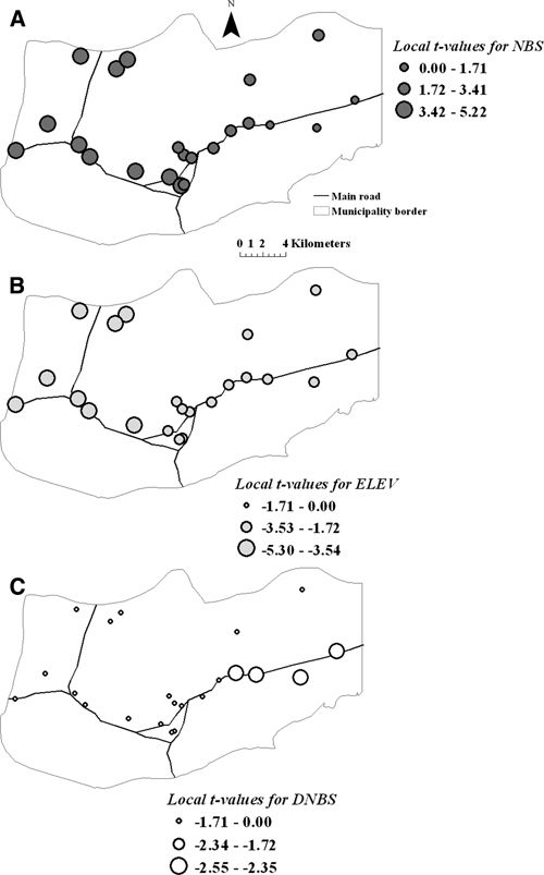
The t-values of regression coefficients for number of breeding sites -NBS- (A), elevation -ELEV- (B), and distance to the nearest breeding site -DNBS- (C), in the local GWR models of 2007.

Predicting malaria persistence.

The GWR on malaria persistence resulted in adjusted R² ranging from 0.54 (2007) to 0.83 (2002), whereas global regression accounted for 33% (2006) to 83% (2002; Table 4). Local spatial GWR models did not show a significant improvement in explaining variation in malaria persistence for every year over the performance of corresponding global OLS regressions (Table 4). Local GWR R² estimates (Figure 4A) varied from 81% to 92%. On average, OLS models showed that increased human population density (e.g., OLS model [2002]: β estimate ± SE [6 × 10⁻⁶ ± 2 × 10⁻⁵], t = 2.40, P < 0.05), lower elevations (e.g., OLS model [2002]: β estimate ± SE [0.001 ± 4 × 10⁻⁴], t = −3.34, P < 0.05), and proximity to mosquito aquatic habitats (e.g., OLS model [2002]: β estimate ± SE [9 × 10⁻⁵ ± 3 × 10⁻⁵], t = −2.90, P < 0.05) were significantly and independently associated with the number of consecutive weeks with malaria during the year. However, GWR models showed considerable heterogeneity in the contribution of these variables to the geography of malaria persistence (Figure 4B–D). In particular, distance to the nearest aquatic habitat of An. aquasalis was not significant everywhere (Figure 4D), only in the hot spots. In predicting malaria persistence across years, the GLMM results converged to those derived using the OSL and GWR models (data not shown).

Table 4.

Model validation and main results of the ordinary least squares regression (OLS) and geographically weighted regression (GWR) models of malaria persistence (IP) in northeastern Venezuela

Model (year)	AICc	R2	ANOVA
	OLS† | GWR†	OLS | GWR	F-value
2001	10.45 | 10.816	0.56 | 0.60	3.06
2002	4.15 | 9.115	0.83 | 0.83	1.19
2003	13.25 | 29.812	0.65 | 0.76	2.59
2004	26.45 | 72.68	0.37 | 0.76	4.65*
2005	9.15 | 11.715	0.62 | 0.69	2.91
2006	16.95 | 17.314	0.33 | 0.58	4.50*
2007	39.95 | 37.915	0.41 | 0.54	3.22

Model variables were population density, terrain elevation, number of aquatic habitats, and distance to the nearest breeding site.

^*P < 0.05.

^†DF of OLS and GWR residuals, respectively.

Figure 4.

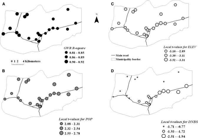
(A) Spatial variation of local R² values or percentage of malaria persistence explained by local GWR models during 2002. (B) The t values of regression coefficients for population (POP), (C) elevation (ELEV), and (D) distance to the nearest breeding site (DNBS) in the local models.

Discussion

Spatially explicit local analyses.

In this study, local spatial statistics were used to test the spatial dependency in the patterns of malaria transmission, detect pockets of disease (Figure 1, Table 2), and identify the relevant spatial scale at which local epidemiology of malaria occurs. Furthermore, although this study relied on a small number of observations, local spatially explicit models (GWR) enabled us to explain variations in hot spots based on environmental variables (Figures 3 and 4) and greatly improved predictions of malaria risk (Table 3, Figure 2) compared with OLS models. Additionally, local spatial predictive models gave more accurate representation of the local variation in P. vivax incidence than the global OLS models by incorporating, detecting, and accounting for spatial non-stationarity (Table 3). Indeed, our results showed that there is significant spatial variation in the relationship between malaria incidence and environmental variables.

Hot spots of malaria.

Malaria risk was highly focal and more prevalent in the central and eastern part of the municipality, where up to 11 malaria hot spots (out of 29 villages) were identified (Tables 1 and 2; Figure 1). Local transmission in these disease pockets accounted for most malaria transmission (73–86%) in the region (Figure 1), suggesting that even at this small spatial scale (~300 km²), the risk of malaria varied widely (Tables 1 and 2). The analysis of retrospective data allowed us to discern that clusters of cases were not transient across space but consistent during all the years, indicating that the area running from the center to the east of the municipality has been a long-standing source of P. vivax transmission in the region. Our results coincided with earlier findings in a small coastal area of northeastern Venezuela where only 40% of human settings accounted for most of the prevalence, incidence, and persistence of P. vivax in the region.³

Factors influencing malaria incidence.

Overall, local and global spatial analyses identified some landscape features influencing the local intensity of malaria in hot spots. The number of An. aquasalis pre-adult habitats within 1 km radius, a proxy for adult female mosquito occurrence and density, was highly predictive of malaria risk in the region. If it is assumed that adult females tend to aggregate around places where they oviposit, then people living near a cluster of water bodies where mosquitoes oviposit would be at higher risk of getting infective Anopheles bites compared with people living in villages further away. At a finer extent, however, the predictive strength of this variable varied across space, as detected by the local spatial models (Figure 3A), where the variable was a poor predictor of malaria incidence in the eastern hot spots. The differences observed in the predictive strength of this variable at different spatial scales (homogeneous at global scale and heterogeneous at finer level) show the ability of the local model to adequately identify the non-stationarity of the process under study. A lower density of mosquito breeding sites was observed in eastern hot spots compared with those areas near the other hot spots (Figure 1). Therefore, although mosquito production site aggregation close to human settlements accounted for “pockets” of disease transmission within this region, other factors operating at local (proximity to aquatic habitats) or greater scale (elevation) explained malaria incidence in the eastern hot spots. Moreover, proximity to water where mosquitoes oviposit, whether these aquatic habitats were less than 1 km, increased the risk of malaria in those eastern hot spots when distance was assessed locally but not globally, where this relevant relationship was missed. Most of the clusters of An. aquasalis habitats next to the central hot spots were small bodies of freshwater (e.g., ponds, springs, and water channels); by contrast, large areas of coastal mangrove swamp forests, freshwater herbaceous swamps or clear-cut marsh forests were located between 1 and 3 km from the eastern hot spots. Thus, people living up to ~3 km of those water bodies are also more exposed to the bites of infected An. aquasalis than those living far away. Our results agreed with previous findings that proximity to mosquito aquatic habitat is a risk factor for malaria.^3,29–32 Proximity to Anopheles production sites has been previously associated with increased adult mosquito density and malaria prevalence.^33,34 The heterogeneous distribution of larval habitats produces large variations in vector-host contact over relatively short distances,³⁰ whereas the abundance of the biting mosquito population away from those breeding sites reflects dispersal and survival of mosquitoes. Formally, in malaria epidemiology, the vector-host contact is expressed as the annual entomologic inoculation rate (EIR), or the expected number of infectious bites per person per day or per year. Hence, it would be interesting to test if the EIR is higher in the central and eastern hot spots compared with the other villages located at low-lying western elevations, where malaria incidence was always relatively low.

Surprisingly, terrain elevation, which is a variable operating at a large scale in the landscape, was a poor predictor of malaria according to the global analyses, although high malaria incidence existed in those settlements located at low altitudes and on gentle slopes (Figure 1). Nevertheless, when this topographic factor was locally assessed, it showed a high degree of correlation with P. vivax infections in the region (Figure 3B). The local model, again, adequately identified the local heterogeneity of the process under study. Although P. vivax infections were not found above 130 m altitude, it was also true that not all the villages localized below that elevation always had high malaria incidence. That heterogeneity could explain the lack of significance of elevation in global models. Lower incidence of malaria is expected at higher elevations because the completion of the mosquito life-cycle critically depends on the availability of aquatic habitats, with flat areas providing more aquatic habitats than steep ones. Additionally, elevation has a limiting effect on the dispersal of Anopheles. Lower elevation in altitudinal geographic gradients has been identified as a risk factor for malaria in previous studies.^31,34

Vector dispersal is another critical aspect in the local spatial epidemiology of malaria.³⁰ The actual adult flight range of An. aquasalis is unknown, but the potential flight range of Anopheles females in the Neotropics may range from 500 to 5,000 m (effective and potential range).³⁵ Adult mosquitoes (Anopheles) may fly up to 5 km, but half of the flights are within a 1 km radius.³⁶ The flight range of An. gambiae s.l., the main vector of malaria in Africa, has been characterized as ranging from 350 m³⁷ to 1.5 km.³⁸ Indeed, malaria transmission risk decreases over distances between 0.5 and 4 km in different suburban and rural settings.^3,34,39 Interestingly, our results on the distance at which the largest value of disease clustering was found and the entomologic risk factor identified here suggest that an underlying spatial process of malaria transmission is acting at distances between 1 and 5 km, and this could be the result of the flight range (effective and potential) of An. aquasalis in the study area. Regarding mosquito survival, it would be interesting to test if proximity to tall, dense vegetation such as mangrove forests promotes higher adult survival of An. aquasalis (providing more resting sites to the flying adults) around the eastern hot spots compared with mosquitoes from central hot spots, where the vegetation is scarce.

Factors influencing malaria persistence.

Significant variability in malaria persistence was accounted for in the hot spots where malaria transmission occurred most of the year. At local and global levels, malaria persistence was associated with higher human population density and lower elevations, but at a local scale (Figure 4), malaria persistence was mainly associated with proximity to aquatic habitats. Consequently, although high local levels of transmission are likely in each hot spot, because of the presence of suitable conditions, sustained and persistent malaria cases were observed only in some localities with specific human population levels.

Additionally, we found that malaria cases clustered in time during the first 13 weeks of the years (dry season) in most of the hot spots, followed by deep troughs in incidence during which the seasonal extinction or fadeout of the parasite occurred in all but the four villages mentioned. In those villages, malaria persistence was almost constant (e.g., one locality in the east side) or continuous (e.g., another locality in the central area) throughout the year. As we found previously,³ malaria in this endemic-disease area of Venezuela is seasonal, with the dry season explaining both the high incidence and spread of the disease in the region. Theoretically, there must be a threshold host density below which microparasite transmission cannot persist.⁴⁰ This value in our study area seemed to be < 200 inhabitants, although we found smaller figures (< 50 inhabitants) for malaria persistence in other study regions of this area of northeastern Venezuela.³ In our study, villages along the main road had significantly more malaria than villages along secondary roads, although the variable main road by itself was not a good predictor of malaria in the models. It would be interesting to evaluate by using metapopulation models⁴¹ whether P. vivax persists regionally in this area because of the physical (landscape features such as the main road) and functional (human dispersal) connectivity of infected hosts.

Implications for malaria control.

In this study, we showed that local transmission of malaria is highly heterogeneous at a small scale, with disease foci made of localities with cases where there may not be autochthonous transmission (cold spots), foci with high or persistent transmission (hot spots), and foci with moderate-to-low local transmission (cool spots) where the infection would disappear by itself if the locality were isolated.² Recent studies suggest that a large reduction in malaria transmission is feasible using targeted control when the heterogeneity and spatial scale of malaria are correctly identified.^4,5,42,43 Hence, we hypothesize that causing a simultaneous and drastic reduction of malaria transmission in the hot spots during the dry seasons will prompt a subsequent fadeout of malaria in the cool spots, and will eliminate cases in cold spots.^3,40 Therefore, mapping the risk of malaria based on fine-grained maps of villages and local An. aquasalis larval habitats (up to 3 km) would be a practical idea for planning interventions in northeastern Venezuela. The heterogeneity and spatial variation in the relationship between malaria incidence and the An. aquasalis aquatic habitats reported here as risk factors would enable the use of various control methodologies to manage the immature mosquito populations.

References

- 1.World Health Organization . World Malaria Report 2008. Geneva: World Health Organization; 2008. [Google Scholar]
- 2.Macdonald G. The Epidemiology and Control of Malaria. London: Oxford University Press; 1957. [Google Scholar]
- 3.Barrera R, Grillet ME, Rangel Y, Berti J, Aché A. Temporal and spatial patterns of malaria reinfection in north-eastern Venezuela. Am J Trop Med Hyg. 1999;61:784–790. doi: 10.4269/ajtmh.1999.61.784. [DOI] [PubMed] [Google Scholar]
- 4.Smith DL, McKenzie FE, Snow RW, Hay SI. Revisiting the basic reproductive number for malaria and its implications for malaria control. PLoS Biol. 2007;5:0531–0542. doi: 10.1371/journal.pbio.0050042. [DOI] [PMC free article] [PubMed] [Google Scholar]
- 5.Carter R, Mendis KN, Roberts D. Spatial targeting of interventions against malaria. Bull W Health Org. 2000;78:1401–1411. [PMC free article] [PubMed] [Google Scholar]
- 6.Ostfeld RS, Glass GE, Keesing F. Spatial epidemiology: an emerging (or re-emerging) discipline. Trends Ecol Evol. 2005;20:328–336. doi: 10.1016/j.tree.2005.03.009. [DOI] [PubMed] [Google Scholar]
- 7.Pavlovsky EN. The Natural Nidality of Transmissible Disease. Urbana: University of Illinois Press; 1966. [Google Scholar]
- 8.Kitron U. Landscape ecology and epidemiology of vector-borne diseases: tools for spatial analysis. J Med Entomol. 1998;35:435–445. doi: 10.1093/jmedent/35.4.435. [DOI] [PubMed] [Google Scholar]
- 9.Real LA, Biek B. Spatial dynamics and genetic of infectious diseases on heterogeneous landscapes. J R Soc Interface. 2007;4:935–948. doi: 10.1098/rsif.2007.1041. [DOI] [PMC free article] [PubMed] [Google Scholar]
- 10.Fortin MJ, Dale MRT. Spatial Analysis: A Guide for Ecologists. New York: Cambridge University Press; 2005. [Google Scholar]
- 11.Legendre P. Spatial autocorrelation: problem or new paradigm? Ecology. 1993;74:1659–1673. [Google Scholar]
- 12.Clennon JA, King CH, Muchiri EM, Kariuki HC, Ouma JH, Mungai P, Kitron U. Spatial patterns of urinary schistosomiasis infection in a highly endemic area of coastal Kenya. Am J Trop Med Hyg. 2004;70:443–448. [PubMed] [Google Scholar]
- 13.Kleinschmidt I, Bagayoko M, Clarke GPY, Craig M, Le Sueur D. A spatial statistical approach to malaria mapping. Int J Epidemiol. 2000;29:355–361. doi: 10.1093/ije/29.2.355. [DOI] [PubMed] [Google Scholar]
- 14.Kleinschmidt I, Sharp BL, Clarke GPY, Curtis B, Fraser C. Use of generalized linear mixed models in the spatial analysis of small-area malaria incidence rates in KwaZulu Natal, South Africa. Am J Epidemiol. 2001;153:1213–1221. doi: 10.1093/aje/153.12.1213. [DOI] [PubMed] [Google Scholar]
- 15.Getis A, Ord JK. The analysis of spatial association by use of distance statistics. Geogr Anal. 1992;24:189–206. [Google Scholar]
- 16.Fotheringham AS, Brunsdon C, Charlton M. Geographically Weighted Regression: The Analysis of Spatially Varying Relationships. Chichester, UK: John Wiley and Sons; 2002. [Google Scholar]
- 17.Rubio-Palis Y, Zimmerman RH. Ecoregional classification of malaria vectors in the neotropics. J Med Entomol. 1997;34:499–510. doi: 10.1093/jmedent/34.5.499. [DOI] [PubMed] [Google Scholar]
- 18.Berti J, Zimmerman R, Amarista J. Adult abundance, biting behavior and parity of Anopheles aquasalis Curry 1932 in two malarious areas of Sucre state, Venezuela. Mem Inst Oswaldo Cruz. 1993;88:363–369. doi: 10.1590/s0074-02761993000300004. [DOI] [PubMed] [Google Scholar]
- 19.Cáceres JL. Malaria antes y después de la cura radical masiva en el estado Sucre, Venezuela. Bol Dir Malariol San Amb. 2008;48:83–90. [Google Scholar]
- 20.Grillet ME. Environmental factors associated with the spatial and temporal distribution of Anopheles aquasalis and Anopheles oswaldoi in wetlands of an endemic malaric area in north-eastern Venezuela. J Med Entomol. 2000;37:231–238. doi: 10.1603/0022-2585-37.2.231. [DOI] [PubMed] [Google Scholar]
- 21.Pérez H. El Paludismo por Plasmodium vivax y los desafíos del tratamiento adecuado y oportuno. Bol Dir Malariol San Amb. 2004;44:1–8. [Google Scholar]
- 22.Szklo M, Nieto FJ. Epidemiology: Beyond the Basics. Gaithersburg, MD: Aspen Publishers, Inc; 2007. [Google Scholar]
- 23.Berti J, Zimmerman R, Amarista J. Spatial and temporal distribution of anopheline larvae in two malarious areas in Sucre State, Venezuela. Mem Inst Oswaldo Cruz. 1993;88:353–362. doi: 10.1590/s0074-02761993000300003. [DOI] [PubMed] [Google Scholar]
- 24.Kulldorff M. A spatial scan statistic. Comm Statist Theory Methods. 1997;26:1481–1496. [Google Scholar]
- 25.Getis A, Ord JK. Local spatial autocorrelation statistics: distributional issues and an application. Geogr Anal. 1995;27:286–306. [Google Scholar]
- 26.Waller AW, Gotway CA. Applied Spatial Statistics for Public Health Data. Hoboken, NJ: John Wiley & Sons, Inc; 2004. [Google Scholar]
- 27.Bolker BB, Brooks ME, Clark CJ, Geange SW, Poulsen JR, Stevens MHH, White JS. Generalized linear mixed models: a practical guide for ecology and evolution. Trends Ecol Evol. 2009;24:127–135. doi: 10.1016/j.tree.2008.10.008. [DOI] [PubMed] [Google Scholar]
- 28.Ihaka R, Gentleman R. R: a language for data analysis and graphics. J Comput Graph Statist. 1996;5:299–314. [Google Scholar]
- 29.Rejmankova E, Roberts DR, Pawley A, Manguin S, Polanco J. Predictions of adult Anopheles albimanus densities in villages based on distances to remotely-sensed larval habitats. Am J Trop Med Hyg. 1995;53:482–488. doi: 10.4269/ajtmh.1995.53.482. [DOI] [PubMed] [Google Scholar]
- 30.Le Menach A, McKenzie FE, Flahault A, Smith DL. The unexpected importance of mosquito oviposition behavior for malaria: non-productive larval habitats can be sources for malaria transmission. Malar J. 2005;4:1–11. doi: 10.1186/1475-2875-4-23. [DOI] [PMC free article] [PubMed] [Google Scholar]
- 31.Ernst KC, Adoka SO, Kowuor DO, Wilson ML, John CC. Malaria hotspot areas in a highland Kenya site are consistent in epidemic and non-epidemic years and are associated with ecological factors. Malar J. 2006;5:1–10. doi: 10.1186/1475-2875-5-78. [DOI] [PMC free article] [PubMed] [Google Scholar]
- 32.Bøgh C, Lindsay SW, Clarke SE, Dean A, Jawara M, Pinder M, Thomas CJ. High spatial resolution mapping of malaria transmission risk in the Gambia, West Africa, using landsat TM satellite imagery. Am J Trop Med Hyg. 2007;76:875–881. [PubMed] [Google Scholar]
- 33.Trape JF, Lefebvrezante E, Legros F, Ndiaye G, Bouganali H, Druilhe P, Salem G. Vector density gradients and the epidemiology of urban malaria in Dakar, Senegal. Am J Trop Med Hyg. 1992;47:181–189. doi: 10.4269/ajtmh.1992.47.181. [DOI] [PubMed] [Google Scholar]
- 34.Barrera R, Grillet ME, Rangel Y, Berti J, Aché A. Estudio eco-epidemiológico de la reintroducción de malaria en el nororiente de Venezuela mediante Sistemas de Información Geográfica y Sensores Remotos. Bol Dir Malariol San Amb. 1998;38:14–30. [Google Scholar]
- 35.Cova-Garcia P. Notas Sobre los Anofelinos de Venezuela y su Identificación. Caracas, Venezuela: Editorial Grafos; 1961. [Google Scholar]
- 36.Service MW. Mosquito (Diptera: Culicidae) dispersal–the long and short of it. J Med Entomol. 1997;34:579–588. doi: 10.1093/jmedent/34.6.579. [DOI] [PubMed] [Google Scholar]
- 37.Costantini C, Li SG, DellaTorre A, Sagnon N, Coluzzi M, Taylor CE. Density, survival and dispersal of Anopheles gambiae complex mosquitoes in a West African Sudan savannah village. Med Vet Entomol. 1996;10:203–219. doi: 10.1111/j.1365-2915.1996.tb00733.x. [DOI] [PubMed] [Google Scholar]
- 38.Thomson MC, Connor SJ, Quinones ML, Jawara M, Todd J, Greenwood BM. Movement of Anopheles gambiae s.l. malaria vectors between villages in The Gambia. Med Vet Entomol. 1995;9:413–419. doi: 10.1111/j.1365-2915.1995.tb00015.x. [DOI] [PubMed] [Google Scholar]
- 39.Clarke SE, Bøgh C, Brown RC, Walraven GEL, Thomas CJ, Lindsay SW. Risk of malaria attacks in Gambian children is greater away from malaria vector breeding sites. Trans R Soc Trop Med Hyg. 2002;96:499–506. doi: 10.1016/s0035-9203(02)90419-0. [DOI] [PubMed] [Google Scholar]
- 40.Anderson RM, May RM. Infectious Diseases of Humans: Dynamics and Control. Oxford, UK: Oxford University Press; 1992. [Google Scholar]
- 41.Grenfell BT, Harwood J. Metapopulation dynamics of infectious diseases. Trends Ecol Evol. 1997;12:395–399. doi: 10.1016/s0169-5347(97)01174-9. [DOI] [PubMed] [Google Scholar]
- 42.Woolhouse ME, Dye C, Etard JF, Smith T, Charlwood JD, Garnett GP, Hagen P, Hii JLK, Ndhlovu PD, Quinnell RJ, Watts CH, Chandiwana SK, Anderson RM. Heterogeneities in the transmission of infectious agents: implications for the design of control programs. Proc Natl Acad Sci USA. 1997;94:338–342. doi: 10.1073/pnas.94.1.338. [DOI] [PMC free article] [PubMed] [Google Scholar]
- 43.Greenwood BM. Control to elimination: implications for malaria research. Trends Parasitol. 2008;24:449–454. doi: 10.1016/j.pt.2008.07.002. [DOI] [PubMed] [Google Scholar]