

Abstract
To quantify spatial protein-protein proximity (colocalization) in paired microscopic images of two sets of proteins labeled by distinct fluorophores, we showed that the cross-correlation and the autocorrelation functions of image intensity consisted of fast and slowly decaying components. The fast component resulted from clusters of proteins specifically labeled, and the slow component resulted from image heterogeneity and a broadly-distributed background. To better evaluate spatial proximity between the two specifically labeled proteins, we extracted the fast-decaying component by fitting the sharp peak in correlation functions to a Gaussian function, which was then used to obtain protein-protein proximity index and the Pearson's correlation coefficient. We also employed the median-filter method as a universal approach for background reduction to minimize nonspecific fluorescence. We illustrated our method by analyzing computer-simulated images and biological images.
Introduction
Protein-protein interactions are of great importance in many biological processes and functions. Fluorescence microscopy is an essential tool in biological research and is often used to identify interacting proteins. Due to limited resolution, it is not yet possible to locate associated proteins directly. Instead, colocalization between two fluorescently-labeled proteins, referred to here as protein-protein proximity, is widely used to map and quantify protein-protein interactions. Protein proximity analysis in fluorescence microscopy typically involves a pair of dual color images, in which each color labels one type of protein. A high level of colocalized signals indicates close proximity of the two proteins of interest, which may suggest interactions between them.
Development of computer technology has made the colocalization analysis of digital images a fast and easily accessible approach to study protein-protein interactions. Among various strategies of colocalization analysis, one of the simplest methods is to overlay the dual color (for example, red and green images) and to assess the amount of overlaid yellow pixels as the indication of interaction (1,2). Colocalization can also be quantified by various approaches, such as the Pearson's correlation coefficient rp (3,4), the overlap coefficient, and the Manders' colocalization coefficients (5), the intensity correlation quotient (6), automatic thresholding method (7), and image cross-correlation spectroscopy (ICCS) (8–11).
Ideally, quantitative colocalization analysis should be able to find the fraction of the colocalized proteins in each channel. However, most quantitative approaches are unable to produce reliable estimation of this fraction even for the simplest computer-simulated images. For example, the Manders' colocalization coefficient of molecules labeled with red dye Mred is defined to be the ratio of the integrated intensity of colocalized red pixels to the total intensity of all red pixels (5). This approach has the obvious drawback that it almost always exaggerates the magnitude of colocalization because of randomly overlapped red and green pixels. When the number density of molecules is large, Manders' coefficient approaches to one even for two completely uncorrelated images.
Biological images are heterogeneous, because specific labeling is not spatially randomly distributed but instead concentrated in discrete subcellular compartments, and cells have spatial patterns and boundaries. Existing quantitative methods can easily generate false colocalization values due to image heterogeneity, because in colocalization analysis one is comparing two images of the same cell, and thus spatial similarities must exist to some extent. These similarities may be counted as colocalization and the colocalization value is therefore overestimated. In practice, one could reduce the influence of image heterogeneity by cropping the image and analyzing small areas, but the uncertainty of the result will increase, as most quantitative methods are by nature statistical and a smaller area results in a relatively smaller sample size (11). Another important issue is background reduction. Various backgrounds, such as nonspecific fluorescence and detector noises, are inevitable in fluorescence imaging. Although the influence of spatially white random noise can be relatively easily measured and reduced by numerical techniques (10,12), the nonspecific fluorescence is much more cumbersome to deal with. One could reduce the contribution of nonspecific fluorescence by estimating its statistical properties on control samples, and then subtract it from the measured samples (12), but this time-consuming method suffers from the large variability of cells. The routinely used procedure to reduce background is thresholding. The often arbitrarily chosen threshold, however, introduces great human bias in determination of colocalization coefficients, which can be quite sensitive to threshold values.
Among existing approaches, ICCS can find the portion of colocalized molecules in each channel when image heterogeneity and background are negligible. In this article we propose an improved version of ICCS, which was designed to minimize the influence of image heterogeneity and broadly distributed background. We observed that, in typical images, the colocalization of proteins decreased drastically when the alignment of the two images was shifted, although there was also a slow-decaying component of correlation caused by image heterogeneity and possibly broad background. We calculated the spatial correlation functions (with respect to x, y shift) and extracted the short-range component from the slow-decaying, long-range component. The former component alone was used in valuating colocalization. False colocalization, the result of image heterogeneity, was effectively removed. In background reduction, rather than choosing different threshold values for different images, we employed the median filter technique to minimize nonspecific fluorescence. This technique provided a universal approach for background reduction. We successfully applied this method on both computer-simulated images and biological images. The protein-protein proximity index (PPI) values were proven to be able to yield good estimation to the fraction of colocalized molecules.
Methods
Fast-decaying component extraction
Images are analyzed following the steps below:
-
1.
Perform alignment adjustment by shifting images to reach maximum correlation. If the adjustment shift value is unreasonably large, however, it may indicate that there is no colocalization, and the observed correlation is only due to background and fluctuation.
-
2.
Calculate the correlation functions of Gkl using Eq. 13.
-
3.
Make a contour plot for each correlation function. Usually the fast-decaying component Skl shows itself as a sharp peak on top of the background Bkl if significant colocalization exists.
-
4.
For each correlation function, choose a straight line through zero. The choice of the direction of the line should make the shallow component drop gently, so that the sharp and shallow components can be better distinguished.
-
5.
Through the straight line, fit the correlation function values by a sum of two Gaussian functions
| (1) |
where r is the pixel shift along the line. W and B are the width of the sharp and shallow component, respectively, and W < B. The Gaussian function was selected to fit the sharp peak because the PSF can be well approximated to this function. The Gaussian function also works well for the shallow component. According to Eq. 15, a successful fit of the sharp peak due to colocalization should yield W ≈ full width at half-maximum of PSF. We call this nonlinear fit a double-Gaussian fit.
-
6.
The estimated PPI values are then given by the ratios among the fitted fast component heights of the correlation functions
| (2) |
and the Pearson's coefficient
We will illustrate the above procedures with the analysis of computer-simulated images and biological images in later sections.
Median filter
We will show later in the article that low signal/noise ratio (SNR) may cause error in PPI estimation. In this study we used a median filter to remove nonspecific fluorescence to avoid using arbitrarily chosen threshold values. The median filter is often used in image processing to remove the spatial white noise. Typical high-resolution images show proteins labeled in clusters surrounded by large areas of nonspecific background. In this condition, the median filter background reduction method will estimate the background value at each pixel by calculating the median value of an n × n square centered at this pixel, with n being at least five times larger than the cluster size. We propose that this large square size assures that the median value reflects the background level, which can then be subtracted from the image. The resulting images in our study were almost free from nonspecific background.
Computer simulation
We used computer simulation to generate images with known PPI to test the method. In simulations, the intensity of simulated images was initially set to all zero, and protein clusters were then thrown in as point sources, each generating an intensity distribution according to a Gaussian PSF. The maximum intensity of each molecule was varied according to the Poisson distribution. The number of proteins was precisely controlled, and thus the exact PPI values were known. The specifically labeled clusters distinguished themselves from the nonspecifically labeled ones by that they were much brighter. The intensity ratio between a specifically labeled cluster and a nonspecifically label one was set to ∼5:1. Random noise was generated by the absolute value of Gaussian random numbers.
Cell labeling and image acquisition
Examples are given for isolated heart myocytes, astrocytes from neonatal mice in primary culture, and transfected human embryonic kidney 293 cell (HEK 293T). Proteins were labeled with specific monoclonal (anti-mouse) and polyclonal antibodies (anti-rabbit). Isolated cells were fixed with 4% paraformaldehyde in 0.1 M Na2HPO4 and 23 mM NaHPO4 (pH 7.4) at room temperature for 20 min, and permeabilized with 0.2% Triton-X 100. Nonspecific binding was blocked for 30 min at room temperature using 10% goat or donkey serum in phosphate-buffered saline, pH 7.4, containing 0.2% Triton X-100 to permeabilize the cells. Double labeling was achieved incubating the cells with polyclonal and monoclonal antibodies (5–10 μg/mL) incubated overnight (at 4°C). Cells were washed, incubated (1 h, room temperature) with secondary Abs Alexa 488 anti-rabbit IgG and Alexa 594 anti-mouse IgG1 (2 μg/mL), washed again and mounted with Prolong (Molecular Probes, Eugene, OR). Stacks of images were typically acquired by optically sectioning cells every 0.1 μm at 0.058 μm per pixel (see Figs. 2, 4, 6, and Fig. 7, later in article) or 0.029 μm per pixel (see Fig. 5, later in article) with a confocal microscope using a 60×, 1.4 NA oil immersion objective. Photomultiplier sensitivity was adjusted to avoid saturation.
Figure 2.
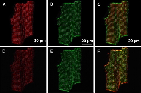
Computer-simulated images based on real biological images. (A) Image (1600 × 1600) of a heart cell where the ryanodine receptor (RyR) was labeled. (B) Image (1600 × 1600) of the same cell where the estrogen receptor α (ERα) was independently labeled. (C) Overlay of images from A and B. (D and E) Computer-simulated images based on A and B, respectively. PPI was set to PD = 0.4 and PE = 0.2. (F) Overlay of images from D and E.
Figure 4.
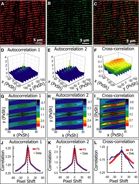
Analysis of images of a heart cell from mouse where ryanodine receptor (RyR) and estrogen receptor α (ERα) were independently labeled. (A) Cropped image (578 × 578) of RyR channel. See Fig. 2A for full image. (B) Cropped image (578 × 578) of ERα channel. See Fig. 2B for full image. (C) Overlay of A and B. (D–F) Three-dimensional plots of the cross-correlation and autocorrelation as functions of pixel shift. (G–I) Two-dimensional plots of the cross-correlation and autocorrelation functions, and the line (dotted) through which the nonlinear fit is performed. (J–L) Fitting the cross-correlation and autocorrelation function along the line to the sum of two Gaussian functions. The cross-correlation function does not have a sharp peak, indicating that colocalization is nonexistent. See Table 3.
Figure 6.
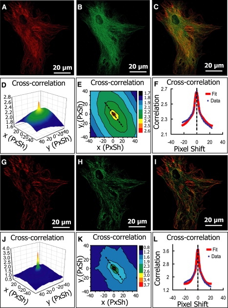
Analysis of images of a mouse brain cell (astrocyte) where two different proteins were independently labeled. (A) MaxiK-α channel (1520 × 1520). (B) α-tubulin channel (1520 × 1520). (C) Overlay of A and B. (D–F) Cross-correlation function and the nonlinear fit; estimated PPI is 0.56 for MaxiK-α, 0.51 for α-tubulin, and Pearson's coefficient is 0.63. (G–L) Equivalent analysis after median-filter background reduction. PPI is 0.37 for MaxiK-α, 0.47 for α-tubulin, and Pearson's coefficient is 0.42.
Figure 7.
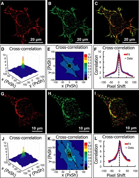
Analysis of images of a human embryonic kidney 293 cell (HEK 293T) where c-Src tyrosine kinase and serotonin receptor subtype 5-HT2AR were coexpressed and independently labeled. (A) c-Src channel after median filter processing (1070 × 1070). (B) 5-HT2AR channel after median-filter processing (1070 × 1070). (C) Overlay of A and B. (D–F) Cross-correlation function and the nonlinear fit; estimated PPI is 0.72 for c-Src, 0.91 for 5-HT2A receptors, and Pearson's coefficient is 0.81. (G–L) Equivalent analysis after the cell membrane was removed. PPI is 0.42 for c-Src, 0.55 for 5-HT2AR, and Pearson's coefficient is 0.48. Lower PPI values inside the cell indicate that c-Src and 5-HT2AR are more strongly colocalized on cell membrane.
Figure 5.
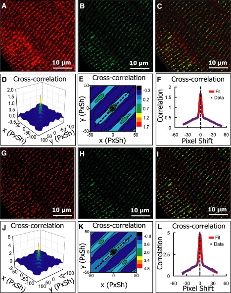
Analysis of images of a mouse heart cell where two different proteins were independently labeled. (A) Cropped image (1250 × 1250) of ryanodine receptor (RyR) channel. (B) Cropped image (1250 × 1250) of α1C calcium channel (α1C). (C) Overlay of A and B. (D–F) The cross-correlation function and the nonlinear fit as described in Fig. 1; estimated PPI is 0.33 for RyR and 1.21 for α1C, and Pearson's coefficient is 0.63. (G–L) Equivalent analysis after median filter background reduction. PPI is 0.55 for RyR, 0.76 for α1C, and Pearson's coefficient is 0.64.
Theory
Model
We consider a pair of two-dimensional images with intensity I1(x, y) and I2(x, y), labeling protein 1 and 2, respectively. The intensity can be decomposed into four components,
| (3) |
where k = 1, 2 and
-
1.
Ck(x, y) (k = 1, 2) is the interacting (colocalized) component, resulting from molecules of protein k that are associated with the other type of protein,
-
2.
Fk(x, y) is the noninteracting component, generated by free molecules of protein k,
-
3.
Nk(x, y) is the product of nonspecific fluorescence, and
-
4.
Rk(x, y) is the random noise.
Our goal is to find the fraction of interacting molecules for both protein 1 and 2, described by PPI P1 and P2. For simplicity we only discuss one-to-one binding (variable binding stoichiometry was discussed in (10)), and the PPI is then defined as
| (4) |
where nc is the number of interacting (colocalized) molecules, and (k = 1, 2) is the number of free molecules of protein k.
We consider each molecule as a point light source. If the point-spread function (PSF) is p(x, y), the ith molecule generates a density distribution p(x − xi, y − yi)ti on the image, where ti is the intensity at position (xi, yi), whose value is determined by various factors such as the quantum yield of fluorophores, the collection efficiency, and the detector gain. Any component J in Eq. 3, except for the random noise, can be expressed as
| (5) |
where summation is over all molecules generating J. The spatial average intensity is
| (6) |
where n is the number of molecules generating J. We use 〈.〉 to denote spatial average and the overbar to denote the operation of averaging over molecules. If position of molecules (xi, yi) is a random variable with probability distribution f(x, y), the variance of J is
| (7) |
where
is the convolution of the PSF p(x, y) and the spatial distribution f(x, y) of molecules. The first term in the right-hand side of Eq. 7 accounts for the spatial distribution of molecules. In the special case that the spatial distribution is uniform, we have (p∗f)(x, y) = 〈p〉, and
| (8) |
The assumption
is essential to image correlation spectroscopy (ICS) (10,12). From Eqs. 7 and 8, one can see that this assumption is only valid when the spatial distribution of molecules is uniform (homogeneous image). In typical fluorescence images, image heterogeneity produces significant effects, and must be taken into account.
Principle of ICCS
The correlation coefficients are defined as
| (9) |
where k, l = 1, 2. In this definition, the product of mean values rather than covariance is used in the denominator for convenience to derive PPI. Note that this definition can give correlation coefficients >1. ICCS use
| (10) |
to estimate P1 and P2. For short-ranged PSF p, we have 〈p2〉 ≫ 〈p〉2. Under the assumption that the spatial distributions of proteins of interest are uniform, and neglecting nonspecific fluorescence and random noise, the correlation coefficients can be formulated as
| (11) |
The PPI are then estimated by
| (12) |
Comparing the above equation to Eq. 4, one can see that the accuracy of the estimate needs a sharp distribution of t1 and t2, and also p1(x, y) ≈ p2(x, y). Various factors, notably the counting noise of detector, may cause a distribution of t1 and t2 and thus cause an underestimation of PPI. In usual dual-color fluorescence microscopy, the PSFs of two channels are practically equal. However, when threshold is applied, p1 and p2 can be effectively changed. Unequal PSF in each channel may also produce distorted results in ICCS.
Correlation function and background reduction
We define correlation function with varying pixel shift (u, v) as
| (13) |
where G11 and G12 are the autocorrelation functions, and G12 is the cross-correlation function. Note that Gkl(0, 0) = rkl. Random noise, nonspecific fluorescence, and image heterogeneity all have their influence on the correlation functions. Random noise can be greatly reduced by image processing techniques such as deconvolution and the median filter. One can also measure the mean value and the variance of random noise directly and perform background correction according to these values. Because random noise is not spatially correlated, the contribution of its variance in Eq. 9 can also be eliminated by extrapolation (10,12), because
when (u, v) ≠ 0, one can use to calculate rkl and eliminate the variance term of random noise. Nonspecific fluorescence is much more difficult to deal with. Unlike random noise, its statistical properties depend on the particular cells under observation and are hard to reliably predetermine, especially when direct labeling is used. Nonspecific fluorescence usually has lower intensity than specific fluorescence and can be reduced by thresholding. In this article, we use the median filter technique to minimize nonspecific fluorescence.
One can observe that, as the alignment of the two images is shifted, the magnitude of colocalization decreases sharply, although there is another component decaying much more gently. This intuition can be formulated mathematically as follows: If the components in Eq. 3 are mutually independent, and 〈R1(x, y)R2(x + u, y + v)〉 = 0 when (u, v) ≠ 0. Using fC(x, y), , and to denote the spatial distribution of colocalized proteins, noninteracting proteins, and nonspecifically labeled molecules in the kth channel (k = 1, 2), respectively, then we have
| (14) |
where
| (15) |
and
| (16) |
where is the number of molecules generating nonspecific fluorescence in channel k. Because in a confocal microscope the PSF is short-ranged, and the spatial distributions of the molecules fC, , and typically have much broader distribution, S12 is much narrower than B12. Therefore, one has a fast-decaying component S12 and a slow-decaying component B12. (If, however, the spatial distribution of molecules is comparable or even narrower than the PSF, one should not expect colocalization analysis to provide accurate information about protein-protein correlation.) Nonlinear fitting techniques can then be used to extract the component S12. Similarly, one can decompose the autocorrelation functions into a fast-decaying component Skk and a slow-decaying component Bkk (k = 1, 2).
Assuming 〈Rk〉 ≪ 〈Ik〉, the correlation coefficients can be estimated by
| (17) |
This equation is very similar to Eq. 12, except that we only use the fast-decaying component Skl in correlation functions to derive PPI. The Pearson's correlation coefficient is estimated by
| (18) |
We have not considered that proteins tend to form clusters, which may have size comparable to the PSF. In this case, the above discussion can still be applied by approximating each cluster to be a single point source. The maximum intensity t for each cluster is then a function of the number of labeled molecules inside the cluster, and ts of the specific component is ≫tn of the nonspecific component, because the nonspecific labeling occurs with much lower probability. The PSF convolutes with the spatial distribution within a cluster, generating an effective PSF of that cluster. As an approximation, we assume that, in image k, all clusters have the same effective PSF pk; Eq. 17 needs to be slightly modified as
| (19) |
SNR is what we call specific-to-nonspecific ratio defined as
| (20) |
The Pearson's correlation coefficient remains the same as in Eq. 18. One can see from Eq. 19 that the estimated PPI is a good approximation to the real values only if both images have negligible nonspecific components, or SNR1 ≈ SNR2. If the two images have a high level of nonspecific labeling and the SNR values are significantly different, then the PPI estimation is skewed, though the Pearson's correlation coefficient rp is not affected. In this case, background reduction process, which is discussed in the next section, has to be done before calculation of PPI.
Results
Computer-simulated images
Many simulated images were analyzed and we show two typical examples in Fig. 1. A pair of images with a spatial pattern and high SNR ≈ 10 (very little nonspecific fluorescence) are shown in Fig. 1, A and B. Their overlay is displayed in Fig. 1 C. The real PPI values are PA = 0.20 and PB = 0.71. Fig. 1 D shows the landscape of the cross-correlation function (mesh), which consists of two clearly distinguishable components—a shallow background reflecting the spatial pattern and a sharp peak on top that accounts for colocalization. The landscape is also shown in Fig. 1 E as a contour plot, together with a straight line (dotted), through which the nonlinear fit is performed. The cross-correlation values through the line were nicely fitted by the sum of two Gaussian functions, illustrated in Fig. 1 F. The same procedure were repeated for the autocorrelation function of each image, and the fitted height of the sharp peaks was then used to calculate the estimation of PPI. The result was PA = 0.22 and PB = 0.75—in excellent agreement with the real values. Without decomposition of the fast and the slow components, however, the PPI values would be exaggerated by the spatial pattern: PA = 0.56 and PB = 0.94 (calculated by ICCS with image scrambling (11)). This proves that our method was very effective in removing the influence of image heterogeneity. In Table 1, results of the PPI method and other previous methods are compared (the overlap coefficient and the Manders coefficient were calculated by the Just Another Colocalization Plugin (http://rsbweb.nih.gov/ij/plugins/track/jacop.html); calculation in ICCS used image scrambling (11)). One can see that previous methods all greatly exaggerate colocalization because of the same spatial pattern the two images have.
Figure 1.
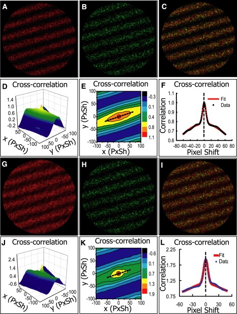
Analysis of computer-simulated images. (A and B) Pair of simulated images with known PPI values and high SNR. (C) Overlay of images from A and B. (D) Three-dimensional plot of the cross-correlation as a function of pixel shift (PxSh). The peak at the center is due to colocalization and the rest to the nonuniform pattern. (E) Two-dimensional contour plot of the cross-correlation function. The straight line (dotted) through the center shows where the double-Gaussian fit is performed. (F) Double-Gaussian fit of the cross-correlation function (normalized). The height of the sharp peak, together with the heights of the sharp peaks on autocorrelation functions (not shown in this figure), are used to estimate the PPI values. The estimation is in excellent agreement to the known values. See Table 1. (G and H) Simulated images resulted from adding unequal amount of nonspecific background to A and B. (I) Overlay of images from G and H. (J) Three-dimensional plot of the cross-correlation function of the median-filtered images. (K) Two-dimensional contour plot of the cross-correlation function. (L) Double-Gaussian fit along the straight line shown in K. The sharp peaks are used to generate better-estimated PPI values than previous approaches. See Table 2.
Table 1.
Comparison of colocalization analysis methods for simulated images with high SNR in Fig. 1, A and B
| PPI A to B | PPI B to A | Correlation | |
|---|---|---|---|
| Real value | 0.20 | 0.71 | 0.38 |
| Pearson's coefficient | N/A | N/A | 0.73 |
| Overlap coefficient | 0.13 | 5.11 | 0.83 |
| Manders' coefficient | 0.98 | 1.00 | N/A |
| Costes' approach | 1.00 | 0.96 | N/A |
| ICCS (image scrambled) | 0.56 | 0.94 | N/A |
| This article | 0.22 | 0.75 | 0.41 |
To test the method under the influence of nonspecific fluorescence, we used two images with different level of nonspecific background (shown in Fig. 1, G and H). The SNR values were 0.16 for Fig. 1 G and 7.0 for Fig. 1 H, whereas the real PPI values were unchanged from the previous example. If background reduction were not performed, our method would yield PG = 0.12 and PH = 1.20, failing to give reasonable estimate for PPI; however, the Pearson's correlation coefficient rp = 0.36 would still be an excellent estimation (the real value is ), as predicted by the theory. The median filter was able to remove most of the background, and the estimated PPI values of the median-filtered images were PG = 0.31 and PH = 0.49, close to the real values. In Table 2, we again compare the PPI method to other methods. One can still see that previous methods usually exaggerate colocalization due to image heterogeneity.
Table 2.
Comparison of colocalization analysis methods for simulated images with low SNR in Fig. 1, J and K
| PPI J to K | PPI K to J | Correlation | |
|---|---|---|---|
| Real value | 0.20 | 0.71 | 0.38 |
| Pearson's coefficient | N/A | N/A | 0.54 |
| Overlap coefficient | 0.12 | 3.33 | 0.64 |
| Manders' coefficient | 0.83 | 0.84 | N/A |
| Costes' approach | 0.72 | 0.68 | N/A |
| ICCS (image scrambled) | 0.51 | 0.57 | N/A |
| This article | 0.31 | 0.49 | 0.41 |
We were able to make our simulation more realistic by using real biological images as the layout of computer simulation. In Fig. 2, A and B we display a pair of biological images of a mouse heart cell where the ryanodine receptor (RyR) and the estrogen receptor α (ERα) were independently labeled. This pair of images (cropped) will be used as the first example in the analysis of biological images in this article (see Fig. 4), in which we will show that RyR and ERα do not colocalize. In computer simulation, the protein clusters were distributed according to the intensity distribution of the biological image used as the layout, producing a simulated image that resembles the biological image on which the simulation was based. In Fig. 2, D and E, we show the simulated images using Fig. 2, A and B as their layouts, respectively. Although colocalization does not exist in the original biological images, one can add colocalization in computer simulations. The amount of artificial colocalization can be precisely controlled, and the simulated images can be used to test colocalization analysis methods. In Fig. 3 A, we show the performance of several quantitative colocalization analysis methods over a broad range of colocalization values. The concentration ratio of two species also varies greatly. It is obvious that the method described in this article produced the best results, whereas other methods all tend to exaggerate the value of colocalization, especially when the colocalization value is low. We have mentioned that the choice of the straight line in the contour plot should follow the direction where the shallow component drops slowly. In Fig. 3 B, line 1 (solid) satisfies the above criterion, whereas line 2 (dash) does not. Fig. 3 C shows that fitting along line 1 yields a better result than line 2, and that the PPI result is not sensitive to the length of the fitting line.
Figure 3.
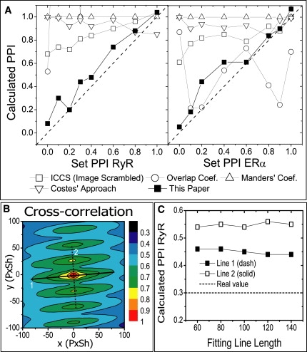
Analysis of computer-simulated images based on biological images. (A) Comparison of quantitative colocalization analysis method over a broad range of colocalization value and concentration ratio, for computer-simulated images using Fig. 2, A and B, as layout. The set (PRyR, PERα) values are (0, 0), (0.1, 0.9), (0.2, 0.1), (0.4, 0.2), (0.3, 0.6), (0.4, 0.2), (0.6, 1), (0.8, 0.4), and (1, 0.8). Results of a better method should form a line closer to the Set PPI = Calculated PPI value (dash). (B) Contour plot of the cross-correlation function of one of the simulated images. Double-Gaussian fit could be performed along either line 1 (solid) or line 2 (dash). (C) Impact of fitting line choice to PPI result. The length of fitting line has little effect, but one needs to choose line 1 to obtain a better estimate to the real PPI value.
Biological images
For biological images, we first show an example of two labeled proteins that show no evidence of being associated. We selected in a mouse heart cell the RyR that localized in the terminal cisternae of the sarcoplasmic reticulum (14) (Fig. 4 A, after cropping and processed by the median filter) and the ERα that is located in different compartment along the transverse T-tubules (15) (Fig. 4 B, after cropping and processed by the median filter). The distribution of proteins in these images clearly formed a spatial pattern of the T-tubules. Very little colocalization is shown in the overlay (Fig. 4 C), contrary to what existing quantitative methods predicted (Table 3). In Fig. 4, D–I, we show correlation functions of the images, and one can see that only autocorrelations show sharp peaks (the fast component), whereas the cross-correlation does not, indicating that the colocalization identified by other methods is not real but caused by image heterogeneity. This is further confirmed by Fig. 4, J–L, where the nonlinear fit nicely identified the sharp component in the autocorrelation functions, but failed to find it in the cross-correlation function. We forced the double-Gaussian fit by fixing the width of the sharp component to be that of the autocorrelation functions, and obtained PA ≈ 0.08 and PB ≈ 0.06.
Table 3.
Comparison of colocalization analysis methods on images of ryanodine receptor (Fig. 4A) and estrogen receptor α (Fig. 4B)
| PPI A to B | PPI B to A | Correlation | |
|---|---|---|---|
| Pearson's coefficient | N/A | N/A | 0.35 |
| Overlap coefficient | 0.15 | 1.66 | 0.50 |
| Manders' coefficient | 0.81 | 0.81 | N/A |
| Costes' approach | 0.59 | 0.49 | N/A |
| ICCS (image scrambled) | 0.32 | 0.37 | N/A |
| This article | 0.08 | 0.06 | 0.07 |
Our second example illustrates the use of a median filter as an effective background reduction method. Fig. 5 shows the analysis of two images of a mouse heart cell where two different proteins that are known to be associated, RyR and α1C calcium channel (α1C), were separately labeled (14) (RyR in Fig. 5, A and G, and α1C in Fig. 5, B and H). The overlay of the images (Fig. 5, C and I) cannot decisively tell us whether colocalization exists. The original two images (Fig. 5, A and B) had very different SNRs, and the application of the PPI method (Fig. 5, D–F) yielded unrealistic PPI values: PA = 0.33 for RyR, and PB = 1.21 for α1C. The estimated Pearson's correlation coefficient was rp = 0.63. After median filter processing (Fig. 5, G and H), the nonspecific fluorescence in the images were removed, and the PPI method yielded reasonable results: PG = 0.55 for RyR and PH = 0.76 for α1C (Fig. 5, J–L). After the median-filter processing, the Pearson's correlation coefficient was estimated to be rp = 0.64. This value almost remained unchanged compared to the value before the median-filter processing.
In the third example, we show the analysis of images with partial colocalization. In Fig. 6 we show two cropped images from a mouse brain cell (astrocyte) where two different proteins, the α-subunit of Ca2+ and voltage-dependent large conductance K+ channels (MaxiK-α) and α-tubulin, were separately labeled. These proteins are known to be associated (16). The astrocyte cells have a complex shape, which might induce false colocalization. The estimated PPI for original images was PA = 0.56 for MaxiK-α and PB = 0.51 for α-tubulin. After median-filter processing, the estimate PPI dropped to PG = 0.37 for MaxiK-α and PH = 0.47 for α-tubulin. The median-filter processing did not significantly change the PPI values, because the original images had similar SNRs. These results indicate that MaxiK-α and α-tubulin are partially colocalized in astrocytes. Again, previous methods tend to overestimate the value of colocalization. For example, the ICCS with image scrambling yields PG = 0.56 and PH = 0.59; the Costes' approach yields PG = 0.72 and PH = 0.82; and the Manders' coefficients are MG = 0.82 and MH = 0.84.
The last example shown in Fig. 7 illustrates the analysis of images that were double-labeled with c-Src tyrosine kinase (Fig. 7 A) and serotonin (5-HT) receptor subtype 5-HT2AR (Fig. 7 B) in coexpressed HEK 293T. These proteins highly colocalize to the cell membrane, facilitating functional coupling (17). In Fig. 7, A–C, we show images processed by the median-filter method, and the PPI values were estimated to be PA = 0.72 for c-Src and PB = 0.91 for 5-HT2AR. The Pearson's coefficient was 0.81. Colocalization is not necessarily homogeneous inside cells. In Fig. 7, G–I, we roughly removed the membrane part of the HEK 239T cell, and the remaining area was found to have lower PPI values: PG = 0.42 for c-Src and PH = 0.55 for 5-HT2AR. The Pearson's coefficient diminished to 0.48. These results suggest that the association between 5-HT2A receptors and c-Src is more likely to happen on HEK 239T membranes. Some other methods may not be able to detect the above difference, because they also give fairly high estimates for the interior region. For example, the Manders' coefficients are MA ≈ MB ≈ 0.9 for uncropped images and MG ≈ MH ≈ 0.8 for cropped ones. The difference is too small to draw a decisive conclusion.
Summary and Discussion
In this article, we have presented a novel method to analyze protein-protein proximity, also referred as colocalization, in dual-color fluorescence microscopic images. Colocalization analysis is widely used in biological research but existing methods have not been satisfactory. For example, the overlay method is limited by its qualitative nature and biased by the user selection of appropriate threshold. Other quantitative strategies involve using scatter plots or second-order histograms (4), which also rely on visual identification of correlation or repulsion. Many quantitative approaches have also been proposed, but they all have their limitations. Pearson's correlation coefficient rp is readily applicable to colocalization analysis (3,4), but it is difficult to interpret small or negative value of rp, and one value of rp is incomplete to quantify the colocalization of two species. The overlap coefficient and the Manders' colocalization coefficient (5) were proposed by Manders and collaborators to quantify colocalization in both species. However, the overlap coefficient has the drawback that it only produces reasonable result when the two channels have similar intensity, and the Manders' coefficient is very sensitive to background noise (18). Li et al. developed the intensity correlation quotient to quantify both correlation and repulsion (6), but similar to the Pearson's coefficient, this quotient is also a single value that changes nonlinearly with respect to the portion of colocalized molecules and thus is hard to interpret, especially when the absolute value of the quotient is small. Costes et al. (7) invented an automatic threshold method, which lacks solid theoretical foundation, and was reported to fail to give a fair estimate when the molecule density was high (10).
Fluorescence correlation spectroscopy has found its applications in various scientific studies. Image correlation spectroscopy (ICS) was introduced as a more rapid alternative to fluorescence correlation spectroscopy (19). ICS measures spatial variations of fluorescence images rather than temporal fluctuations in the sample, and it has been applied to the measurement of protein aggregation in the plasma membrane (12,20). Cross-correlation analysis was incorporated with ICS, termed as image cross-correlation spectroscopy (ICCS), to analyze protein-protein colocalization (8,9). According to a recent summary by Comeau et al. (10), ICCS is an excellent strategy when applied to homogeneous images with relatively high magnitude of colocalization, but failed on heterogeneous images and images with low colocalization, because of the difficulty in the three-dimensional Gaussian nonlinear fit. These authors extended the use of ICCS by scrambling and padding the images (11). This approach can make the Gaussian fit easier to perform but is vulnerable to false colocalization induced by image heterogeneity.
In this article, we showed that the correlation functions usually consist of a fast decaying component corresponding to colocalization and a slowly changing component due to heterogeneity and nonspecific fluorescence. The mathematical formalization validated the usage of ICCS on heterogeneous images. For inhomogeneous images, we introduced double-Gaussian nonlinear fit to extract the fast decaying component. The double-Gaussian fit substituted the more difficult and unstable three-dimensional nonlinear fit, performed on a line where the fast and slow component were easy to distinguish.
Compared to existing approaches, our method has the following advantages:
First, one is able to calculate the PPI that has a clear biological meaning: They are an excellent approximation to the fractions of colocalized molecules, if nonspecific fluorescence is negligible.
Second, our method is free from false identification of colocalization induced by image heterogeneity. This is particularly important when there is no colocalization or the colocalization value is low.
Third, the median-filter method provides a universal and stable approach for background reduction. The PPI method can serve as a powerful microscopy tool to map and quantify association of macromolecular complexes and their dynamic changes in biological processes.
The strategy we present in this article is not intended as a substitute for Förster resonance energy transfer (FRET). FRET is much harder to implement but has the advantage that it can achieve resolution well below the conventional microscopy diffraction limit. FRET is mainly used in expression systems where the expressed proteins are tagged with fluorophores (e.g., cyan fluorescent protein or yellow fluorescent protein). In native tissues, proteins are typically first tagged with a primary antibody and subsequently with a secondary fluorescent antibody. A much better approach is to use fluorescent-tagged antibodies, but they are not always available. In any case, one would measure FRET between two fluorescent primary antibodies or secondary antibodies, which could introduce uncertainty (21,22).
Acknowledgments
This work was supported by National Institutes of Health grants No. HL088640 (to E.S.), No. HL054970 (to L.T.), and No. HL089876 (to M.E.), and American Heart Association Fellowship No. 0825273F (to R.L.).
References
- 1.Fox M.H., Arndt-Jovin D.J., Robert-Nicoud M. Spatial and temporal distribution of DNA replication sites localized by immunofluorescence and confocal microscopy in mouse fibroblasts. J. Cell Sci. 1991;99:247–253. doi: 10.1242/jcs.99.2.247. [DOI] [PubMed] [Google Scholar]
- 2.Dutartre H., Davoust J., Chavrier P. Cytokinesis arrest and redistribution of actin-cytoskeleton regulatory components in cells expressing the ρGTPase CDC42Hs. J. Cell Sci. 1996;109:367–377. doi: 10.1242/jcs.109.2.367. [DOI] [PubMed] [Google Scholar]
- 3.Manders E.M., Stap J., Aten J.A. Dynamics of three-dimensional replication patterns during the S-phase, analyzed by double labeling of DNA and confocal microscopy. J. Cell Sci. 1992;103:857–862. doi: 10.1242/jcs.103.3.857. [DOI] [PubMed] [Google Scholar]
- 4.Demandolx D., Davoust J. Multicolor analysis and local image correlation in confocal microscopy. J. Microsc. 1997;185:21–36. [Google Scholar]
- 5.Manders E.M., Verbeek F.J., Aten J.A. Measurement of colocalization of objects in dual-color confocal images. J. Microsc. 1993;169:375–382. doi: 10.1111/j.1365-2818.1993.tb03313.x. [DOI] [PubMed] [Google Scholar]
- 6.Li Q., Lau A., Stanley E.F. A syntaxin 1, Gα(o), and N-type calcium channel complex at a presynaptic nerve terminal: analysis by quantitative immunocolocalization. J. Neurosci. 2004;24:4070–4081. doi: 10.1523/JNEUROSCI.0346-04.2004. [DOI] [PMC free article] [PubMed] [Google Scholar]
- 7.Costes S.V., Daelemans D., Lockett S. Automatic and quantitative measurement of protein-protein colocalization in live cells. Biophys. J. 2004;86:3993–4003. doi: 10.1529/biophysj.103.038422. [DOI] [PMC free article] [PubMed] [Google Scholar]
- 8.Wiseman P.W., Squier J.A., Wilson K.R. Two-photon image correlation spectroscopy and image cross-correlation spectroscopy. J. Microsc. 2000;200:14–25. doi: 10.1046/j.1365-2818.2000.00736.x. [DOI] [PubMed] [Google Scholar]
- 9.Costantino S., Comeau J.W., Wiseman P.W. Accuracy and dynamic range of spatial image correlation and cross-correlation spectroscopy. Biophys. J. 2005;89:1251–1260. doi: 10.1529/biophysj.104.057364. [DOI] [PMC free article] [PubMed] [Google Scholar]
- 10.Comeau J.W., Costantino S., Wiseman P.W. A guide to accurate fluorescence microscopy colocalization measurements. Biophys. J. 2006;91:4611–4622. doi: 10.1529/biophysj.106.089441. [DOI] [PMC free article] [PubMed] [Google Scholar]
- 11.Comeau J.W., Kolin D.L., Wiseman P.W. Accurate measurements of protein interactions in cells via improved spatial image cross-correlation spectroscopy. Mol. Biosyst. 2008;4:672–685. doi: 10.1039/b719826d. [DOI] [PubMed] [Google Scholar]
- 12.Wiseman P.W., Petersen N.O. Image correlation spectroscopy. II. Optimization for ultrasensitive detection of preexisting platelet-derived growth factor-β receptor oligomers on intact cells. Biophys. J. 1999;76:963–977. doi: 10.1016/S0006-3495(99)77260-7. [DOI] [PMC free article] [PubMed] [Google Scholar]
- 13.Reference deleted in proof.
- 14.Scriven D.R.L., Dan P., Moore E.D.W. Distribution of proteins implicated in excitation-contraction coupling in rat ventricular myocytes. Biophys. J. 2000;79:2682–2691. doi: 10.1016/S0006-3495(00)76506-4. [DOI] [PMC free article] [PubMed] [Google Scholar]
- 15.Ropero A.B., Eghbali M., Stefani E. Heart estrogen receptor alpha: distinct membrane and nuclear distribution patterns and regulation by estrogen. J. Mol. Cell. Cardiol. 2006;41:496–510. doi: 10.1016/j.yjmcc.2006.05.022. [DOI] [PubMed] [Google Scholar]
- 16.Ou J.W., Kumar Y., Toro L. Ca2+- and thromboxane-dependent distribution of MaxiK channels in cultured astrocytes: from microtubules to the plasma membrane. Glia. 2009;57:1280–1295. doi: 10.1002/glia.20847. [DOI] [PMC free article] [PubMed] [Google Scholar]
- 17.Lu R., Alioua A., Toro L. c-Src tyrosine kinase, a critical component for 5-HT2A receptor-mediated contraction in rat aorta. J. Physiol. 2008;586:3855–3869. doi: 10.1113/jphysiol.2008.153593. [DOI] [PMC free article] [PubMed] [Google Scholar]
- 18.Bolte S., Cordelières F.P. A guided tour into subcellular colocalization analysis in light microscopy. J. Microsc. 2006;224:213–232. doi: 10.1111/j.1365-2818.2006.01706.x. [DOI] [PubMed] [Google Scholar]
- 19.Petersen N.O., Höddelius P.L., Magnusson K.E. Quantitation of membrane receptor distributions by image correlation spectroscopy: concept and application. Biophys. J. 1993;65:1135–1146. doi: 10.1016/S0006-3495(93)81173-1. [DOI] [PMC free article] [PubMed] [Google Scholar]
- 20.Nohe A., Petersen N.O. Image correlation spectroscopy. Sci. STKE. 2007;2007:pl7. doi: 10.1126/stke.4172007pl7. [DOI] [PubMed] [Google Scholar]
- 21.Kenworthy A.K. Imaging protein-protein interactions using fluorescence resonance energy transfer microscopy. Methods. 2001;24:289–296. doi: 10.1006/meth.2001.1189. [DOI] [PubMed] [Google Scholar]
- 22.König P., Krasteva G., Kummer W. FRET-CLSM and double-labeling indirect immunofluorescence to detect close association of proteins in tissue sections. Lab. Invest. 2006;86:853–864. doi: 10.1038/labinvest.3700443. [DOI] [PubMed] [Google Scholar]