Abstract
We formulate a technique for the detection of functional clusters in discrete event data. The advantage of this algorithm is that no prior knowledge of the number of functional groups is needed, as our procedure progressively combines data traces and derives the optimal clustering cutoff in a simple and intuitive manner through the use of surrogate data sets. In order to demonstrate the power of this algorithm to detect changes in network dynamics and connectivity, we apply it to both simulated neural spike train data and real neural data obtained from the mouse hippocampus during exploration and slow-wave sleep. Using the simulated data, we show that our algorithm performs better than existing methods. In the experimental data, we observe state-dependent clustering patterns consistent with known neurophysiological processes involved in memory consolidation.
I. INTRODUCTION
The detection of structural network properties has been recently recognized to be of great importance in aiding understanding of the properties of a variety of man-made and natural networks [1–4]. Here, however, two significantly different notions of network structure have to be identified. One is the physical (or anatomical) structure of the network. In this case, community structure refers to groups of nodes within a network which are more highly connected to other nodes in the group than to the rest of the network. Here, multiple techniques exist which utilize a knowledge of the network topology (adjacency matrix) to extract this hidden structure [5–8].
The other type of structure is functional structure, which refers to a commonality of function of subsets of units within the network, generally observed by monitoring the similarities in the dynamics of nodes [9,10]. Thus the structural proximity (i.e existence of physical connection between the network elements) is replaced with the notion of functional commonality (or proximity), which can rapidly evolve based on the observed dynamics. The concept of identifying functional relationships between nodes has been gaining popularity [11–13] as many networks with dynamic nodes (e.g., genetic, internet, neuronal, etc.) exist with the goal of uniting to perform a specific task or function.
In order to successfully capture the (physical or functional) community structure of a network, a clustering algorithm should have two important properties: the ability to detect relationships between nodes in order to form clusters and the ability to determine the specific set of clusters which optimally characterize the network structure. While some clustering methods have been designed to extract the structure directly from the dynamics of the neurons [11,14–18], most methods rely on using a similarity measure to compute distances in similarity space between neurons and then use structural clustering methods to determine the functional groupings [13,19–23]. However, a major problem becomes identifying statistically significant community structures from spurious ones. To achieve this goal, current structural clustering techniques involve an optimization of the network modularity [24,25] or require a prior knowledge of the number of communities [3,5,26–29].
In this paper, we develop a clustering method that does not depend on structural network information but instead derives the functional network structure from the temporal interdependencies of its elements. We refer to this method as the functional clustering algorithm (FCA). The key advantage of this algorithm is that it incorporates a natural cutoff point to cease clustering and obtain the functional groupings without an a priori knowledge of the number of groups. Additionally, the algorithm can be used with a variety of different similarity measures, allowing it to detect functional groupings based on multiple features of the data. While the algorithm is generic and applies to any type of discrete event data, we introduce the algorithm in the context of an application to spike train data as the inspiration for the algorithm comes from neuroscience and spike trains are a simple example of discrete event data.
The brain is a prime example of a system where the physical (anatomical) structure cannot be obtained. The cortex alone contains around 1.5×10¹⁴ tightly packed connections (synapses) and it is clearly impossible to derive any detailed properties of its connectivity. It is not even completely clear that having such a detailed knowledge of the connectivity would be particularly useful in understanding brain function, as it significantly evolves during the lifetime of an individual through such processes as neuronal loss, adult neurogenesis, and constant rewiring (i.e., creation, annihilation, and modulation of synapses). Also, since it is known that brain function is distributed over large neuronal ensembles, or even more globally, between different brain modalities, it becomes imperative to understand how these ensembles self-organize to generate desired functions (movement, memory storage/recall, etc.) [11,30–32]. The advent of techniques that allow the activity of many cells to be simultaneously monitored provides hope for a clearer understanding of these neural codes but also demands novel tools for the detection and characterization of spatiotemporal patterning of this activity.
While it is assumed that these ensembles are formed dynamically [33–36] through spatiotemporal interactions of activity patterns of many individual neurons, the neural correlates of cognition are not well understood. One of the most prominent hypothesis addressing this issue is the temporal correlation hypothesis [37–40]. Namely, it is assumed that correlations between activity pattern of neurons mediate feature binding and thus formation of intermittent functional ensembles in the brain. Thus, functional clustering can potentially be reduced to the identification of temporally correlated groups of neurons.
The paper is organized as follows. We first introduce the functional clustering algorithm, along with a similarity metric designed to detect cofiring events in neural data. We then compare the performance of the algorithm to two existing methods using simulated data and show that it performs better than existing measures. Finally, we demonstrate the application of our algorithm to experimental data exploring progressive memory consolidation in the hippocampus.
II. FUNCTIONAL CLUSTERING ALGORITHM
Here we introduce the FCA which is tailored to detect functional clusters of network elements. The algorithm can be applied to any type of discrete event data, however, this paper will focus only on the application of the algorithm to neural spike train data.
The FCA dynamically groups pairs of spike trains based on a chosen similarity metric, forming progressively more complex spike patterns. We will introduce a similarity measure which is used for the data analyzed in this paper, but any pairwise similarity measure can be chosen. The specific choice of the metric should depend on the nature of the data being analyzed and the type of functional relationships which one chooses to detect.
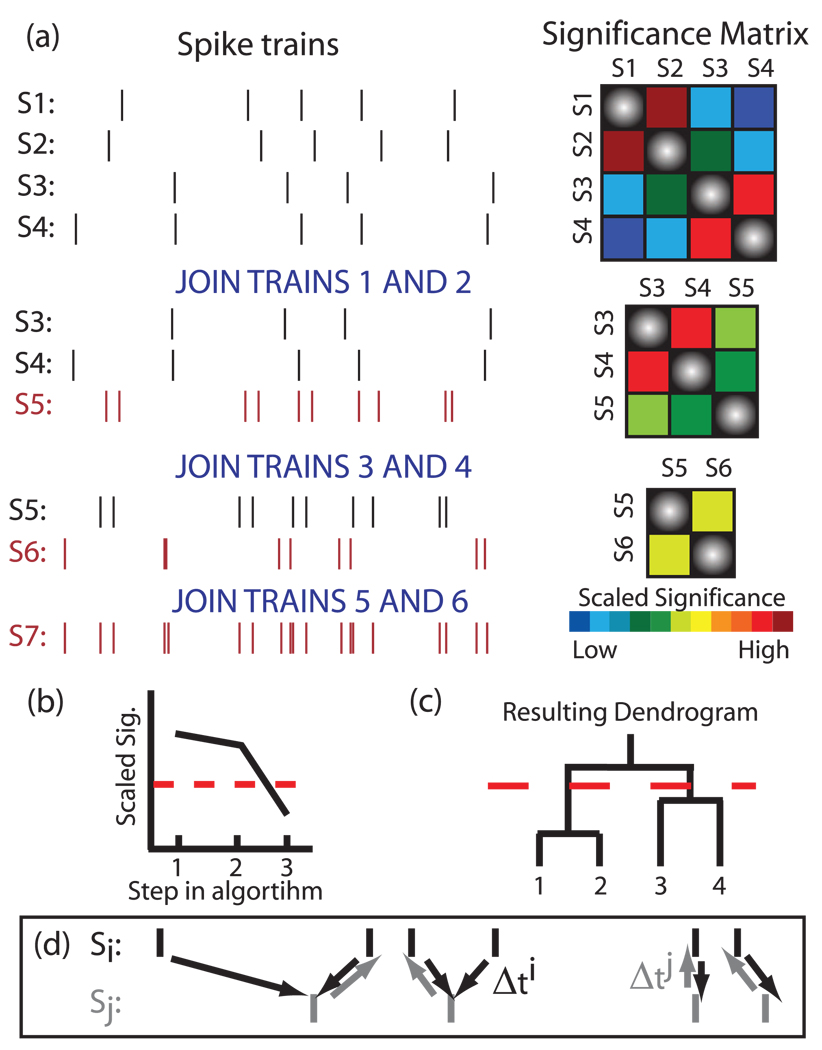
A general description of the FCA is as follows (see the subsequent sections for detailed descriptions and Fig. 1 for a schematic of the algorithm).
FIG. 1.
(Color) Functional clustering algorithm. (a) An example of the algorithm applied to four spike trains. Two trains are merged in each step by selecting the pair of neurons with the highest scaled significance value and effectively creating a new neuron by temporally summing their spike trains. The procedure is repeated until one (complex) spike train remains. (b) We cease clustering when the trains being grouped are no longer significant; here the dotted red line denotes the significance cutoff. (c) The subsequent dendrogram obtained from the FCA. The dotted line denotes the clustering cutoff. (d) Schematic of the average minimum distance between spike trains.
We first create a matrix of pairwise similarity values between all spike trains.
We then use surrogate data sets to calculate 95% confidence intervals for each pairwise similarity. These significance levels are used to calculate the scaled significance between each pair of similarity values (see Sec. II C for the definition of scaled significance).
The pair of trains with the highest significance is then chosen to be grouped together, and the scaled significance of this pair is recorded. A unique element of the FCA is that the two spike trains which are grouped together are then merged by joining the spikes into a single new train [see Fig. 1(a)]. This allows for a cumulative assessment of similarity between the existing complex cluster and the other trains.
The trains which are being joined are then removed, the similarity matrix is recalculated for the new set of trains, new surrogate data sets are created, and a new scaled significance matrix is calculated.
We repeat the joining steps [(3) and (4)], recording the scaled significance value used in each step of the algorithm until the point at which no pairwise similarity is statistically significant, indicating that the next joining step is not statistically meaningful. We refer to this step as the clustering cutoff (dashed red line in Fig. 1). At this point, the functional groupings are determined by observing which spike trains have been combined during the clustering algorithm.
A key advantage of this algorithm is that the ongoing comparison of the similarity metric obtained from the data with that from the surrogates causes the algorithm to have a natural stopping point, meaning that one does not need an a priori knowledge of the number of functional groups embedded in the data. Gerstein et al. [11] also developed an aggregation method based on grouping neurons with significant coincident firings, but this method results in the formation of strings of related neurons which must be further parsed to determine functional groupings. We now discuss the details of the implementation of the FCA in the following sections.
A. Average minimum distance
For the data presented in this paper, we use a similarity metric which we call the average minimum distance (AMD) denoted by Θ to determine functional groupings. The AMD is useful in capturing similarities due to coincident firing between neurons. Note that other metrics could be chosen, depending upon the nature of the recorded data. To compute the AMD between two spike trains Si and Sj, we calculate the distance from each spike in Si to the closest spike in Sj as shown in Fig. 1(d). We then define
| (1) |
where Ni/j is the total number of spikes in Si or Sj, respectively. Finally, we define the AMD between spike trains Si and Sj to be
| (2) |
B. Adjusted average minimum distance
One feature of the FCA is that the similarity associated with each joining step of the algorithm can be compared between different applications of the algorithm. When using the AMD as the chosen similarity measure, we must first introduce a frequency correction during the calculation of the Dij values as this measure scales with the number of spikes in the trains otherwise. (Note that the effect of spiking frequency in the measure is accounted for in the algorithm through the comparison to surrogate data.)
Here, we normalize these distances by the average expected distance obtained from uniformly distributed spike trains having the same spike frequency: , where ΔT is the train length. Thus,
| (3) |
We then define Θ̃, the adjusted average minimum distance ( ) between trains Si and Sj to be
| (4) |
Lower values of the  indicate tighter functional clustering between the cells.
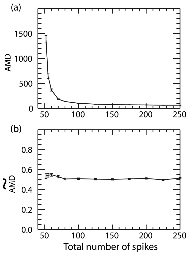
In Fig. 2 we show the average AMD and  values calculated between two random Poisson trains as a function of the total number of spikes within the trains averaged over 100 trials. In this case, one spike train has a constant value of 50 spikes and the other train is varied from 2–200 spikes over a constant window of time. In Fig. 2(a), we show the original AMD calculation between the trains. As expected, the AMD scales approximately as 1/N where N is the total number of spikes. In Fig. 2(b) we show the
  calculated for the same spike trains. One can see that this first-order correction effectively eliminates the dependence on spiking frequency as the measure is approximately constant over all frequencies.
FIG. 2.
(a) AMD and (b)  calculated between two random Poisson trains as a function of the total number of spikes in the trains. One spike train contained a constant number of 50 spikes while the spiking frequency in the other was varied between 2 and 200 spikes. While the AMD scales with the number of spikes in the trains, the
  remains constant as the number of spikes is varied.
C. Calculation of significance
In order to determine the significance between two trains, we create 5000–10000 surrogate data sets and calculate pair-wise similarities for each surrogate set. The surrogate spike trains are created by adding a jitter to each spike in the train. This jitter is drawn from a normal distribution [41], similar to the technique developed by Date et al. [42]. The method of adding jitter to spikes (also known as dithering or teetering) to create surrogate data sets is commonly used when analyzing neural data and has been shown to eliminate correlations between spike timings [43,44]. Creating the surrogate trains in this manner preserves the frequency of each train while keeping the gross properties of the interspike-interval distribution.
We examine the distribution of similarity values and create the cumulative distribution function (CDF) to determine the 95% level of significance. The scaled significance (Fig. 3 and Fig 8) is measured in units defined as the distance from the midpoint of the CDF to the 95% significance cutoff. Thus, a scaled significance value equal to one denotes the 95% significance level, and values higher than one are significant while values lower than one are deemed insignificant.
FIG. 3.
(Color) Performance of the FCA on simulated data. (a) The cross-correlation matrix showing the correlation structure of the simulated data. (b) The scaled significance used in each step of the FCA. The dashed red line denotes the point at below which clustering is no longer significant. (c) Dendrogram resulting from functional clustering. The algorithm easily identifies the correct groups.
FIG. 8.
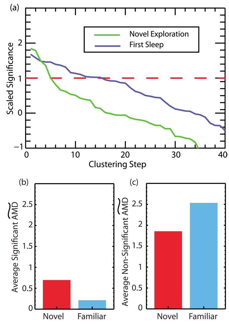
(Color online) (a) The scaled significance used in clustering calculated for novel exploration (0–200s) and the first sleep period (900–1100s). The significance cutoff is shown by the dashed line. The FCA is able to detect the greater number of neurons involved in joint firing known to occur during sleep. (b) Comparison of the  averaged over significant clustering steps from novel exploration and a subsequent familiar exploration. We observe a decrease in this value during the familiar exploration as correlations between neurons become tighter. (c) Comparison of the
  distances averaged over nonsignificant clustering steps during novel and familiar exploration. Here we see an increase in this value during familiar exploration as neurons which were uncorrelated become further decorrelated.
III. COMPARISON TO OTHER ALGORITHMS
In order to verify the performance of the FCA and compare it to that of existing clustering methods, we created simulated spike trains with a known correlation structure. Specifically, we created a set of 100 spike trains derived from a Poisson distribution that consist of four independent groups, 20 spike trains each, and 20 uncorrelated spike trains. The spike trains within these four groups are correlated [see Fig. 3(a)]. To create the correlated groups, we first created a master spike train and used this train to create new trains by randomly deleting spikes from the master train with a certain probability. Thus, the resulting train was also a Poisson process with a firing rate dependent upon the deletion probability. The master train was 5000 time steps long, with each neuron spiking an average of 250 times during the duration of the train. To further randomize the timings of the spikes copied from the master train, we added jitter (drawn from a normal distribution with a standard deviation of 1) to the spike times. Each correlated group was composed of 20 trains from the same master. The average correlation within the group was computed by first calculating the pairwise cross correlations between all trains and then averaging over the group. The firing rate of the independent trains was set to match that of the correlated trains.
We first applied the FCA to the simulated data described above [Fig. 3(b) and Fig. 3(c)] using a jitter drawn from a normal distribution with a standard deviation of 10 to create the surrogate data. In Fig. 3(b), we show the scaled significance at each joining step in the algorithm. The dashed red line marks the significance cutoff (single 95% confidence interval); points above this line are statistically significant and the clustering cutoff is given by the point where the curve drops below this line. Figure 3(c) shows the resulting dendrogram with the dashed red line denoting the clustering cutoff. The algorithm correctly identifies the four groups of neurons as well as the 20 independent neurons.
A. Comparison to the gravitational method
We then compared the performance of the FCA to that of the gravitational method [14–17]. This method performs clustering based on the spike times of neuronal firings by mapping the neurons as particles in N-dimensional space and allowing their positions to aggregate in time as a function of their firing patterns. Particles are initially located along the trace of the N-dimensional space and given a “charge” which is a function of the firing pattern on the neuron. The charge qi on a particle is given by
| (5) |
where K(t)=exp(−t /τ) for t>0 and K=0; otherwise, Tk are the firing times of the neuron, and λi is the firing rate of the neuron normalized so that the mean charge on a particle is zero. The position vector x of the particle is then allowed to evolve based upon the following rule:
| (6) |
where κ is a user defined parameter that controls the speed of aggregation. One then calculates the Euclidean distance between particles as a function of time and looks for particles which cluster in the N-dimensional space (i.e., the distance between the particles becomes small).
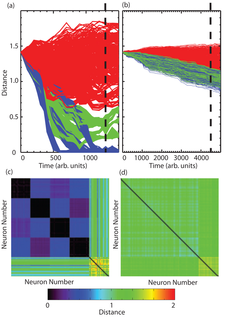
Figure 4 depicts the results of applying the gravitational method to the simulated data described above for cases of high correlation (C ≈ 0.63) within groups [Figs. 4(a) and 4(c)] and also for low correlation (C≈0.13) within clusters [Figs. 4(b) and 4(d)]. In Figs. 4(a) and 4(b) we plot the pairwise distances between particles as a function of time in the algorithm. Blue traces denote distances between intracluster trains, green between intercluster ones, and red between any train and an independent train. To visualize the results of the method, we have sliced these plots as indicated by the dashed vertical line and represent the distances at this point in time as matrices in Figs. 4(c) and 4(d). While, for the case of high correlation between the spike trains, the algorithm separates the four groups correctly [black squares in Fig. 4(c)], one is unable to distinguish between intercluster and intracluster trains for the low correlation case. Further-more, these plots must be visually inspected for the cutoff (i.e., time point at which they stabilize) and the clustering results may significantly depend on its position, as the algorithm has no inherent stopping point and the rate of aggregation is parameter dependent. Even then, the detection of the formed clusters may require the application of an additional N-dimensional clustering algorithm to detect the clusters formed in the N-dimensional space. Another drawback of this method is that as the particles aggregate into clusters, the clusters start interacting due to the nature of the algorithm, causing intercluster distances to become significantly lower than those with random trains, which does not match the correlation structure of the data. The FCA performed the correct clustering of the data for the case of the high correlation and only made an occasional error for data with the low correlation.
FIG. 4.
(Color) Application of the gravitational method to simulated data. [(a) and (b)] Pairwise distances as a function of time in the stimulation for high correlation within clusters (a) and low correlation within clusters (b). Blue traces: intracluster distances; green traces: intercluster distances; and red traces: distances between any train and an independent train. [(c) and (d)] Matrix version of distances for the point in time denoted by the dashed vertical line in (a) and (b), respectively. Note that for the low correlation case, one cannot detect the formation of individual clusters.
B. Comparison to complete linkage and modularity
We next compare the performance of the FCA to a method which maps spiking dynamics onto a structural space and then uses a structural clustering method to determine functional groupings. The structural clustering method used is a standard hierarchical clustering technique called complete linkage. Since this algorithm has no inherent cutoff point at which clustering is stopped, we combine it with a calculation of the weighted modularity [25], which is a commonly used measure to determine the best set of groupings when dealing with hierarchical clustering methods. We have also tried other methods [single-linkage, Girvan and New-man (GN) algorithm [5,19]], but complete linkage gave the best results of the other methods attempted. Please see [19,20] for a review of standard hierarchical clustering techniques.
The complete linkage algorithm again clusters trains based upon a similarity measure. In this algorithm, a similarity matrix is created and the elements with the maximum similarity are joined. However, the clusters are formed through virtual grouping of the elements and there is no recalculation of the similarity measure; the similarity between clusters is simply defined to be the minimum similarity between elements of the clusters. For the data presented in this paper, we use the absolute value of the normalized cross-correlation matrix as our similarity matrix, since this is what is commonly used to do examine community structure in neuroscience applications. To compute this matrix, spike trains are first convolved with a Gaussian kernel and the signal is demeaned (the mean value of the signal is subtracted). The cross correlation is given by
| (7) |
where C is the linear cross-correlation function
| (8) |
Since the complete linkage algorithm has no inherent method of determining the clustering cutoff, we compute the (weighted) modularity [25] for each step of the algorithm. The modularity measure was originally tailored to detect the optimal community structure based upon structural connections between nodes (i.e., adjacency matrix); however it can also be used to detect optimal clustering based on not structural but dynamical relations, where the adjacency matrix is substituted with the correlation matrix. The modularity is given by
| (9) |
where Aij is our similarity matrix, , and δ(ci ,cj)=1 if i and j are in the same community and zero otherwise. The maximum value of the modularity is then used to define the clustering cutoff.
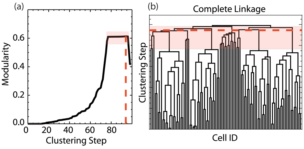
The complete linkage dendrogram is shown in Fig. 5(b) and the modularity for this clustering is plotted in Fig. 5(a). The clustering cutoff is defined as the maximum of the modularity [24,25]; however the scaling of the modularity, even in this simple case, provides ambiguous results. The numerical maximum of the modularity is observed for the clustering step marked by the dashed red line in Fig. 5—significantly above the clustering step that starts linking random spike trains. Even if we relax this definition and assume that the set of high modularity values is equivalent, the exact location of the cutoff is ambiguous as shown by the area enclosed in the transparent red box. Note that the FCA does not have this ambiguity, as the cutoff is quite clear and the algorithm correctly identifies the groups embedded in the spike train data.
FIG. 5.
(Color online) (a) Modularity calculation for the clustering obtained using complete linkage. The transparent red (gray) box marks the ambiguous cutoff area. (b) Dendrogram indicating clustering by complete linkage. Here the clustering cutoff is ambiguous and the algorithm fails to identify the appropriate structure.
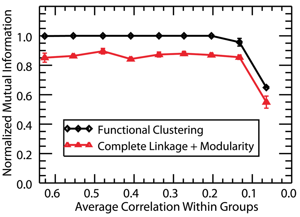
To further explore the performance of the FCA in comparison with complete linkage and modularity, we monitor the performance of both methods for progressively lower correlations within the four clustered groups (Fig. 6). We did not perform this analysis for the gravitational method since that algorithm has no predetermined stopping point and cluster identification must be assessed by the user. As before, the intercluster correlation is controlled through progressive random deletion of spikes from a master train. In order to compare the performance of the two algorithms, it is necessary to compare the obtained clusterings to the known structure of the data. To assess the correctness of the retrieved clusters as compared to the actual structure of the network, we calculate I, the normalized mutual information (NMI) [8,45] as a function of the average correlation within the constructed groups. The NMI is a measure used to evaluate clustering algorithms and determine how well the obtained clustering C′ matches the original structure C. To compute the NMI, one first creates a matrix with c rows and c′ columns, where c is the number of communities in C and c′ is the number of found communities in C′. An entry Nij is defined to be the number of nodes in community i that have been assigned to the found community j. If we denote Ni/j=Σj/iNij and N=ΣijNij then we can define
| (10) |
FIG. 6.
(Color online) Normalized mutual information as a function of average group correlation. The measure takes a maximal value of one when the established clustering structure matches the predetermined groups and I→0 when the obtained clustering structure is independent of the original groupings. Functional clustering identifies the correct group structure for almost all values of correlation while complete linkage and modularity consistently create erroneous structure.
This measure is based on how much information is gained about C given the knowledge of C′. It takes a minimum value of 0 when C and C′ are independent and a maximal value of 1 when they are identical.
In Fig. 6 we use the NMI to compare the obtained clustering with the known structure of the simulated data. As shown in the figure, complete linkage and modularity consistently fail to identify the correct structure. This is because the maximum of the modularity occurs for a point in the algorithm where various independent spike trains have been joined, creating erroneous group structure. However, the FCA correctly identifies neurons for almost all values of correlation. Please note that the 80% level of correctness using complete linkage and modularity for higher intercluster correlation values is due to the fact that we had only 24 independent groups (20 spike trains +4 independent clusters) in the tested network. A higher number of independent neurons would lead to a poorer performance of that method (due to the erroneous grouping of independent neurons) and thus higher relative effectiveness of the FCA.
IV. APPLICATION TO EXPERIMENTAL DATA
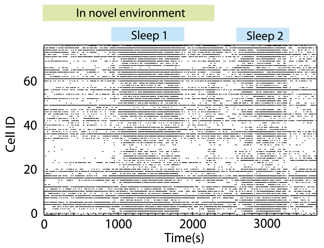
In order to show possible applications of the FCA to real data, we examined spike trains recorded from the hippocampus of a freely moving mouse, using tetrode recording methods [46]. All animal experiments were approved by the University of Michigan Committee on the Use and Care of Animals. In this paper, we focus on the population of pyramidal neurons (77 total; by subregion: 42 CA1, 21 CA2, and 14 CA3). While recording this cell population, the mouse was placed in a novel rectangular track environment. The mouse initially explored the environment by running approximately 20 laps, then settled down, and shortly thereafter fell asleep. A raster plot of this data is shown in Fig. 7. This data set is of interest for two reasons. First, there are established differences in the functional organization of hippocampal networks between active exploration and slow-wave sleep [47]. These include the joint activation of pyramidal cell ensembles at time scales corresponding to gamma frequencies during awake movement [48] and the high-speed replay of pyramidal cell sequences within ripple events that occur preferentially during slow-wave sleep and rest [49]. Second, the mouse learned a new spatial representation during exploration of the novel environment (as indicated by the formation of “place fields” [46]) and the subsequent epoch of slow-wave sleep has been hypothesized to be a period of memory consolidation [50,51] that is presumed to involve alterations in structural and thus functional network connectivity. These structural alterations involve the strengthening of existing monosynaptic connections between the neurons. Furthermore, recent experimental findings have shown that memory consolidation of the neural representation of novel stimuli results in two changes: neurons that are correlated during initial exposure progressively increase their cofiring, while the neurons that have shown a loose relation become further decorrelated [52]. In terms of network reorganization, this should lead to the tightening of the cluster of cells involved in the coding of the new environment and, at the same time, a functional decoupling from the other cells.
FIG. 7.
(Color online) Raster plot of neural data obtained from an unrestrained mouse during exploration of a novel environment and sleep.
Given these functional differences between the various behavioral states of the mouse, we expected to see different clustering patterns during the exploration and sleep phases due to the known differences in network dynamics between these behavioral states.
In Fig. 8(a) we show the scaled significance used in the FCA during the initial exploration as well as the first sleep period. For this data, the jitter amount added to create surrogates was drawn from a normal distribution with a standard deviation of 10s to destroy long term rate correlations between neurons which would arise from the formation of place cells. The cutoff point in the algorithm occurs when the scaled significance drops below the dashed red line. The step in the algorithm at which this cutoff occurs indicates the number of neurons involved in the clustering. Thus if a cutoff occurs for a late (as opposed to early) step in the clustering, more neurons are recruited into the clusters. One can see that there is an increase in the number of significant pairs being clustered during the sleep period (due to the later stage of cutoff), consistent with the increased coactivation of neurons known to occur during sleep ripples.
We then compared the initial exploration of the novel environment to a subsequent exploration of the same environment (after the sleep epochs). Here, we hypothesized that due to memory consolidation and the associated changes in correlations between neurons, we would observe a selective drop in the joining AMD when comparing the initial exposure to a novel environment to a subsequent exposure once the environment has become familiar. This drop should occur for initially small AMD values (initially correlated neurons) as these neurons become further correlated. However, for initially large (insignificant) AMD values, we expect an increase in the AMD values when comparing novel and familiar exploration. This growth occurs as the neurons with low correlations become further uncorrelated.
To assess any changes in the AMD values between initial (novel) and familiar exploration, we examine the  values (see Sec. II B) used in the joining steps of the FCA when applied to data from each epoch. In Fig. 8(b), we show changes in the average
  s used to cluster the neurons for the clustering steps which have a significantly lower
  than that obtained from surrogates (i.e., cofiring cells), during novel exploration and a subsequent familiar exploration. We indeed see that the average
  value is lower for neurons during the familiar exploration indicating that the firing patterns of the neurons are more tightly correlated. Thus, as in the case of [52], the observed decrease of the
  during the subsequent presentation of the novel environment occurs for neurons which fire in the same spatial locations of the maze. In Fig. 8(c), we show the average
  distances for the nonsignificant clustering steps during the novel and familiar exploration. These distances are greater during the familiar exploration as the activity of the neurons having low correlation becomes even less correlated.
V. CONCLUSIONS
In conclusion, we have developed a functional clustering algorithm to perform grouping based on relative activity patterns of discrete event data sets. We applied this algorithm to neural spike train data and have shown that the algorithm performs better than existing ones in simple test cases, using simulated data. Additionally, we showed that the algorithm successfully detects state-related changes in the functional connectivity of the mouse hippocampus. Functional clustering should therefore be a useful tool for the detection and analysis of neuronal network changes occurring during cognitive processes and brain disorders.
Additionally, we would like to emphasize that the algorithm is generic and can be applied to any network whose nodes participate in discrete temporal events. Possible other networks to which the algorithm could be applied include networks of oscillators where the trajectory passes through a Poincaré section, failure events on networks of routers, or fluctuation events in a power grid network. Thus, the functional clustering algorithm is a valuable method for the detection of functional groupings in dynamic network data.
ACKNOWLEDGMENTS
This work was funded by the NSF (S.F.), NIH under Grant No. NIBIB EB008163 (M.Z.), the Whitehall Foundation (J.B.), and the National Institute on Drug Abuse under Grant No. R01 DA14318 (J.B.). The authors would also like to thank the Center for the Study of Complex Systems at the University of Michigan for the use of their computing resources to analyze data in this paper.
References
- 1.Strogatz SH. Nature (London) 2001;410:268. doi: 10.1038/35065725. [DOI] [PubMed] [Google Scholar]
- 2.Albert R, Barabasi AL. Rev. Mod. Phys. 2002;74:47. [Google Scholar]
- 3.Newman MEJ. SIAM Rev. 2003;45:167. [Google Scholar]
- 4.Schwarz AJ, Gozzi A, Bifone A. Magn. Reson. Imaging. 2008;26:914. doi: 10.1016/j.mri.2008.01.048. [DOI] [PubMed] [Google Scholar]
- 5.Girvan M, Newman M. Proc. Natl. Acad. Sci. U.S.A. 2002;99:7821. doi: 10.1073/pnas.122653799. [DOI] [PMC free article] [PubMed] [Google Scholar]
- 6.Leicht EA, Newman MEJ. Phys. Rev. Lett. 2008;100:118703. doi: 10.1103/PhysRevLett.100.118703. [DOI] [PubMed] [Google Scholar]
- 7.Newman MEJ. Proc. Natl. Acad. Sci. U.S.A. 2006;103:8577. [Google Scholar]
- 8.Danon L, Díaz-Guilera A, Duch J, Arenas A. J. Stat. Mech.: Theory Exp. 2005;P09008 [Google Scholar]
- 9.Fingelkurts AA, Fingelkurts AA, Kahkonen S. Neurosci. Biobehav Rev. 2005;28:827. doi: 10.1016/j.neubiorev.2004.10.009. [DOI] [PubMed] [Google Scholar]
- 10.Friston KJ, Frith CD, Liddle PF, Frackowiak RSJ. Cereb. J Blood Flow Metab. 1993;13:5. doi: 10.1038/jcbfm.1993.4. [DOI] [PubMed] [Google Scholar]
- 11.Gerstein GL, Perkel DH, Subramanian KN. Brain Res. 1978;140:43. doi: 10.1016/0006-8993(78)90237-8. [DOI] [PubMed] [Google Scholar]
- 12.Slonim N, Atwal GS, Tkacik G, Bialek W. Proc. Natl. Acad. Sci. U.S.A. 2005;102:18297. doi: 10.1073/pnas.0507432102. [DOI] [PMC free article] [PubMed] [Google Scholar]
- 13.Eldawlatly S, Jin R, Oweiss KG. Neural Comput. 2009;21:450. doi: 10.1162/neco.2008.09-07-606. [DOI] [PMC free article] [PubMed] [Google Scholar]
- 14.Gerstein GL, Perkel DH, Dayhoff JE. J. Neurosci. 1985;5:881. doi: 10.1523/JNEUROSCI.05-04-00881.1985. [DOI] [PMC free article] [PubMed] [Google Scholar]
- 15.Baker SN, Gerstein GL. Neural Comput. 2000;12:2597. doi: 10.1162/089976600300014863. [DOI] [PubMed] [Google Scholar]
- 16.Dayhoff JE. Biol. Cybern. 1994;71:263. doi: 10.1007/BF00202765. [DOI] [PubMed] [Google Scholar]
- 17.Lindsey BG, Gerstein GL. J. Neurosci. Methods. 2006;150:116. doi: 10.1016/j.jneumeth.2005.06.019. [DOI] [PubMed] [Google Scholar]
- 18.Schneidman E, Bialek W, Berry M., II . In: Advances in Neural Information Processing 15. Becker S, Thrun S, Obermayer K, editors. Cambridge: MIT; 2003. pp. 197–204. [Google Scholar]
- 19.Borgatti S. Connections. 1994;17:78. [Google Scholar]
- 20.Boccaletti S, Latora V, Moreno Y, Chavez M, Hwang DU. Phys. Rep. 2006;424:175. [Google Scholar]
- 21.Berger D, Warren D, Normann R, Arieli A, Grun S. Neurocomputing. 2007;70:2112. [Google Scholar]
- 22.Kreuz T, Haas JS, Morelli A, Abarbanel HDI, Politi A. J. Neurosci. Methods. 2007;165:151. doi: 10.1016/j.jneumeth.2007.05.031. [DOI] [PubMed] [Google Scholar]
- 23.Ozden I, Lee HM, Sullivan MR, Wang SSH. J. Neurophysiol. 2008;100:495. doi: 10.1152/jn.01310.2007. [DOI] [PMC free article] [PubMed] [Google Scholar]
- 24.Newman MEJ, Girvan M. Phys. Rev. E. 2004;69:026113. doi: 10.1103/PhysRevE.69.026113. [DOI] [PubMed] [Google Scholar]
- 25.Newman MEJ. Phys. Rev. E. 2004;70:056131. [Google Scholar]
- 26.Fortunato S, Latora V, Marchiori M. Phys. Rev. E. 2004;70:056104. doi: 10.1103/PhysRevE.70.056104. [DOI] [PubMed] [Google Scholar]
- 27.Zhou H. Phys. Rev. E. 2003;67:041908. doi: 10.1103/PhysRevE.67.041908. [DOI] [PubMed] [Google Scholar]
- 28.Newman MEJ. Phys. Rev. E. 2004;69:066133. [Google Scholar]
- 29.Ball GH, Hall DJ. Behav. Sci. 1967;12:153. doi: 10.1002/bs.3830120210. [DOI] [PubMed] [Google Scholar]
- 30.Hebb D. The Organization of Behavior. New York: Wiley; 1949. [Google Scholar]
- 31.Singer W. Neuron. 1999;24:49. doi: 10.1016/s0896-6273(00)80821-1. [DOI] [PubMed] [Google Scholar]
- 32.Zhou CS, Zemanova L, Zamora-Lopez G, Hilgetag CC, Kurths J. New J. Phys. 2007;9:178. [Google Scholar]
- 33.Milner PM. Psychol. Rev. 1974;81:521. doi: 10.1037/h0037149. [DOI] [PubMed] [Google Scholar]
- 34.Engel AK, Singer W. Trends Cogn. Sci. 2001;5:16. doi: 10.1016/s1364-6613(00)01568-0. [DOI] [PubMed] [Google Scholar]
- 35.von der Malsburg C. Curr. Opin. Neurobiol. 1995;5:520. doi: 10.1016/0959-4388(95)80014-x. [DOI] [PubMed] [Google Scholar]
- 36.Singer W. Ann. N.Y. Acad. Sci. 2001;929:123. doi: 10.1111/j.1749-6632.2001.tb05712.x. [DOI] [PubMed] [Google Scholar]
- 37.von der Malsburg C. MPI Biophysical Chemistry Internal Report. 1981 unpublished.
- 38.Gray CM. Neuron. 1999;24:31. doi: 10.1016/s0896-6273(00)80820-x. [DOI] [PubMed] [Google Scholar]
- 39.Singer W. Annu. Rev. Physiol. 1993;55:349. doi: 10.1146/annurev.ph.55.030193.002025. [DOI] [PubMed] [Google Scholar]
- 40.Engel AK, Konig P, Singer W. Proc. Natl. Acad. Sci. U.S.A. 1991;88:9136. doi: 10.1073/pnas.88.20.9136. [DOI] [PMC free article] [PubMed] [Google Scholar]
- 41.Rolston JD, Wagenaar DA, Potter SM. Neuroscience. 2007;148:294. doi: 10.1016/j.neuroscience.2007.05.025. [DOI] [PMC free article] [PubMed] [Google Scholar]
- 42.Date A, Bienenstock E, Geman S. Division of Applied Mathematics, Brown University, Technical Report. 1998 unpublished.
- 43.Shmiel T, Drori R, Shmiel O, Ben-Shaul Y, Nadasdy Z, Shemesh M, Teicher M, Abeles M. J. Neurophysiol. 2006;96:2645. doi: 10.1152/jn.00798.2005. [DOI] [PubMed] [Google Scholar]
- 44.Pazienti A, Maldonado PE, Diesmann M, Grun S. Brain Res. 2008;1225:39. doi: 10.1016/j.brainres.2008.04.073. [DOI] [PubMed] [Google Scholar]
- 45.Fred ALN, Jain AK. Proceedings of 2003 IEEE Computer Society Conference on Computer Vision and Pattern Recognition; pp. 128–133. URL: ieeexplore.iee.org/stamp/stamp.jsp?arnumber=1211462&isnumber27266. [Google Scholar]
- 46.Berke JD, Hetrick V, Breck J, Greene RW. Hippocampus. 2008;18:519. doi: 10.1002/hipo.20435. [DOI] [PubMed] [Google Scholar]
- 47.Buzsáki G, Buhl DL, Harris KD, Csicsvari J, Czéh B, Morozov A. Neuroscience. 2003;116:201. doi: 10.1016/s0306-4522(02)00669-3. [DOI] [PubMed] [Google Scholar]
- 48.Harris KD, Csicsvari J, Hirase H, Dragoi G, Buzsáki G. Nature (London) 2003;424:552. doi: 10.1038/nature01834. [DOI] [PubMed] [Google Scholar]
- 49.Foster DJ, Wilson MA. Nature (London) 2006;440:680. doi: 10.1038/nature04587. [DOI] [PubMed] [Google Scholar]
- 50.Buzsáki G. J. Sleep Res. 1998;7:17. doi: 10.1046/j.1365-2869.7.s1.3.x. [DOI] [PubMed] [Google Scholar]
- 51.Kudrimoti HS, Barnes CA, McNaughton BL. J. Neurosci. 1999;19:4090. doi: 10.1523/JNEUROSCI.19-10-04090.1999. [DOI] [PMC free article] [PubMed] [Google Scholar]
- 52.O’Neill J, Senior TJ, Allen K, Huxter JR, Csicsvari J. Nat. Neurosci. 2008;11:209. doi: 10.1038/nn2037. [DOI] [PubMed] [Google Scholar]


