Metabolica: a statistical research tool for analyzing metabolic networks

Abstract

Steady state flux balance analysis (FBA) for cellular metabolism is used, e.g., to seek information on the activity of the different pathways under equilibrium conditions, or as a basis for kinetic models. In metabolic models, the stoichiometry of the system, commonly completed with bounds on some of the variables, is used as the constraint in the search of a meaningful solution. As model complexity and number of constraints increase, deterministic approach to FBA is no longer viable: a multitude of very different solutions may exist, or the constraints may be in conflict, implying that no precise solution can be found. Moreover, the solution may become overly sensitive to parameter values defining the constraints. Bayesian FBA treats the unknowns as random variables and provides estimates of their probability density functions. This stochastic setting naturally represents the variability which can be expected to occur over a population and helps to circumvent the drawbacks of the classical approach, but its implementation can be quite tedious for users without background in statistical computations. This article presents a software package called Metabolica for performing Bayesian FBA for complex multi-compartment models and visualization of the results.

1 Introduction

The complexity of detailed models of cellular metabolic systems makes their computer implementation a real challenge. The variance in response to stimuli, typical for living organisms, the inevitable inaccuracies in measurements, and the limitations and shortcomings in even the more detailed models make the interpretation of model predictions very delicate, raising the question how representative or reliable any single computed response is. To quantify uncertainties, it is therefore imperative to include statistical and stochastic elements in the models. The design of statistical computational models of cellular metabolism is not a straightforward task because the information available is usually not given in terms of probabilities and likelihoods, thus requiring an interpretative step. The question of how to incorporate the available information becomes even more poignant when the complexity of the mathematical model is not matched by enough quantitative data to identify all model parameters, leading to problems that without additional information do not have a unique solution, or have solutions that are unfeasible or extremely sensitive to perturbations.

The Bayesian statistical framework is particularly well suited for taking into account the variability of the data and model deficiencies and for utilizing qualitative information such as sparsity of the solution. Its effectiveness in the design and analysis of computational models for cellular metabolism has recently been demonstrated ([1, 2, 3, 4, 5, 6, 7]). The algorithmic details that need to be addressed when implementing a Bayesian framework for complex models can be very tedious and require a good knowledge of stochastic methods and scientific computing.

The program package Metabolica is an open source software package written in Matlab, specifically designed for the analysis of multicompartment metabolic systems within a Bayesian framework. It provides a user-friendly interface for specifying the compartmentation of the system and the metabolic pathways of interest. The package then proceeds to set up the governing equations in a Bayesian framework, solves the full Bayesian inference problem by exploring the posterior densities of interest using Markov Chain Monte Carlo (MCMC) sampling and summarizes the results in graphical format, including the autocorrelation diagnostics of the Monte Carlo sampling.

The first release of Metabolica can be used for in silico studies of steady or stationary states of complex spatially lumped compartmentalized metabolic models. The Matlab source code can be downloaded from http://filer.case.edu/ejs49/Metabolica.

In recent years, a number of different approaches for analyzing metabolic networks and accompanying open source program packages, see, e.g., [8, 9, 10, 11, 12, 13, 14], have been published. Methodologically, they are based on techniques like optimization, pathway analysis involving either elementary modes or extreme pathways, graph theory, uniform random sampling, metabolic control analysis, or stochastic simulation based on molecular level chemical master equation. The philosophy behind Metabolica differs substantially from the other existing packages. What makes Metabolica stand apart is the use of statistical models which are based on a stochastic extension of deterministic macroscopic models, as opposed to, e.g., molecular level Markov models. Rather than predicting single outputs that may be dubious because of the instabilities and shortcomings of the model, the program infers on probability densities of the unknowns. Uncertainties in the predictions manifest themselves in the form of large variations of the output predictions. On the other hand, unlike more general Bayesian inference research tools such as WinBUGS [15] or MCSim [16], Metabolica is application specific, providing user friendly tools for constructing the full statistical model starting from plain stoichiometry.

The current version of Metabolica is restricted to steady and stationary state analysis, implying that implicit constraints based on the kinetic expressions of the reactions and transports or on thermodynamics are not included in the model. This is not a restriction of the Bayesian methodology and the dynamic models will be included in later versions of the package.

This article is organized as follows. Section 2 describes the deterministic macroscopic multi-compartment model framework for cellular level metabolism of Metabolica. Section 3 reviews the stochastic extension of the stationary state model that is the basis for constructing simulated experiments with Metabolica. Following the Bayesian statistical paradigm, probability is tantamount to lack of information on the model and the parameters defining it. Section 4 presents the MCMC algorithms and methods to analyze the output and sampler performance. The details associated with constructing the model and running a simulation with Metabolica are addressed in Section 5, and finally, in Section 6, some future visions are outlined.

2 Multi-compartment model

Multi-compartment models provide a flexible way of describing spatially lumped complex systems within a unified framework. Here, we describe the general structure of the multi-compartment models [4, 17, 18, 19], and to make the discussion more tangible, we illustrate it with a three compartment model for skeletal muscle metabolism discussed in detail in [2]. The construction of the model follows the classical paradigm of deterministic modeling of metabolic systems.

The fundamental building blocks of multi-compartment models are the compartments C_ℓ, 1 ≤ ℓ ≤ L. Each compartment may or may not communicate with another compartment.

We associate to each compartment C_ℓ a time dependent state vector C^ℓ = C^ℓ (t) ∈ ℝ^n_ℓ whose components are concentrations of biochemical species in the compartment. The state of the multi-compartment system is then described by the vector

$$\begin{array}{cc}\mathbf{C}=\left[\begin{array}{c}{\mathbf{C}}^1\\ ⋮\\ {\mathbf{C}}^L\end{array}\right]\in {ℝ}^{n_{\text{tot}}},& n_{\text{tot}}=n_1+\cdots +n_L.\end{array}$$

The time evolution of the system is governed by a system of differential equations. To construct the kinetic model, we identify four different mechanisms that may affect the concentrations of biochemical species within a compartment:

1. Intra-compartment reactions, namely the biochemical reactions within the compartment transforming species into others;

2. Transports, occurring either as passive diffusion of a species from one compartment to another, or through the mediation of a carrier which makes it possible for a species to get across an active membrane;

3. Shuttle mechanisms, or interchange of species through membrane-bound reactions; virtual transports of reducing equivalents;

4. Convection or diffusion, where species are carried into or out of the system by the blood flow (convection) or by being diluted via a diffusion process.

Shuttle mechanisms show similarities with carrier-facilitated transports, except that the substrates do not necessarily cross the membranes. Instead, what is exchanged are reducing equivalents, and the shuttle is indeed a multi-compartment reaction. In modeling antiporters as shuttles, it is essential to keep the opposing transport fluxes in balance.

To write the governing equations, we therefore introduce four vectors corresponding to the mechanisms listed above:

• Φ = intra-compartmental reaction fluxes,

• J = transport rates between the compartments,

• Ψ = shuttle fluxes,

• K = convection and/or diffusion fluxes.

In a deterministic model describing the time evolution of the vector of concentrations of metabolites and intermediates, the mass balance equations are of the form

$$\mathbf{D}=V\frac{d\mathbf{C}}{\mathit{\text{dt}}}=\mathrm{S}\mathbf{\Phi }+\mathrm{M}\mathbf{J}+\mathrm{R}\mathbf{\Psi }+\mathrm{Q}\mathbf{K},$$ (1)

where V = [v_ij] is a diagonal matrix, whose nonzero entry v_ii is the effective volume of the host compartment of the species with label i. This model assumes time-invariant compartment volumes and requires a modification, e.g., in the presence of rapid vascular responses to metabolic activity, but is valid under steady or near steady state metabolism. The matrix S = [s_ij] is the stoichiometric matrix, the entry s_ij indicating how many moles of species i is produced (s_ij > 0) or consumed (s_ij < 0) in the jth reaction. The matrix M = [m_ij] indicates if the ith substrate is transported into the compartment by the jth transport (m_ij = 1), if it is transported out (m_ij = −1) or if it is not exchanged at all (m_ij = 0). The matrix R is the stoichiometric matrix of reactions participating in the shuttle mechanisms. Finally, the matrix Q = [q_ij] indicates if the species is subject to convection (q_ij > 0) or not. The convection terms are discussed in further detail in the example below.

Example: To make the discussion more concrete, consider a three compartment model for skeletal muscle metabolism ([2]), where the compartments are blood (b), cytosol (c) and mitochondria (m). In the blood compartment, we identify nine species that are transported by the blood and exchanged with the cytosol domain, see Figure 1. There are no reactions in the blood, nor are there shuttle mechanisms that would involve species in the blood compartment. The convection term is assumed to be proportional to the difference between the arterial and venous blood concentrations, denoted by ${\mathbf{C}}_{\mathrm{a}}^{\mathrm{b}}$ and ${\mathbf{C}}_{\mathrm{v}}^{\mathrm{b}}$, respectively. Therefore, the model in the blood compartment can be written as

$${\mathbf{D}}^{\mathrm{b}}=V^{\mathrm{b}}\frac{d{\mathbf{C}}^{\mathrm{b}}}{\mathit{\text{dt}}}={\mathbf{J}}_{\mathrm{c}\to \mathrm{b}}-{\mathbf{J}}_{\mathrm{b}\to \mathrm{c}}+Q\mathbf{K},\mathbf{K}={\mathbf{C}}_{\mathrm{a}}^{\mathrm{b}}-{\mathbf{C}}_{\mathrm{v}}^{\mathrm{b}},$$ (2)

where V^b is the volume of the blood domain and the scalar Q is the blood flow parameter. The transport terms between blood and cytosol compartments are denoted with the subindex. The concentration vector C^b is related to the arterial and venous values by a mixture model, ${\mathbf{C}}^{\mathrm{b}}=F{\mathbf{C}}_{\mathrm{v}}^{\mathrm{b}}+(1-F){\mathbf{C}}_{\mathrm{a}}^{\mathrm{b}}$, where F is the mixing ratio, 0 < F < 1.

Figure 1.

Three compartment skeletal muscle metabolism model.

In this example we follow 26 biochemical species in the cytosol compartment. No convection is present, but transports of selected species with the blood and mitochondria compartments take place. Furthermore, the glycerol 3-phosphate shuttle, responsible for the transmembrane exchange of reducing equivalents between the cytosol and mitochondria, is present. The cytosolic reactions included in the model are the principal ones in the glycolytic and β-oxidation pathway creatine-phosphocreatine kinase, ATP hydrolysis and adenylate kinase. The dynamic mass balance equations for the cytosol are of the form

$$\begin{array}{lll}{\mathbf{D}}^{\mathrm{c}}& =& V^{\mathrm{c}}\frac{d{\mathbf{C}}^{\mathrm{c}}}{\mathit{\text{dt}}}\\ & =& {\mathrm{S}}^{\mathrm{c}}{\mathbf{\Phi }}^{\mathrm{c}}-{\mathrm{M}}_{\mathrm{c}\to \mathrm{b}}^{\mathrm{c}}{\mathbf{J}}_{\mathrm{c}\to \mathrm{b}}+{\mathrm{M}}_{\mathrm{b}\to \mathrm{c}}^{\mathrm{c}}{\mathbf{J}}_{\mathrm{b}\to \mathrm{c}}-{\mathrm{M}}_{\mathrm{c}\to \mathrm{m}}^{\mathrm{c}}{\mathbf{J}}_{\mathrm{c}\to \mathrm{m}}+{\mathrm{M}}_{\mathrm{m}\to \mathrm{c}}^{\mathrm{c}}{\mathbf{J}}_{\mathrm{m}\to \mathrm{c}}+{\mathrm{R}}^{\mathrm{c}}\mathbf{\Psi },\end{array}$$ (3)

V^c being the effective volume of the cytosol domain and the subscripts in the transport vectors indicating compartments between which the exchange occurs.

In mitochondria we include 21 biochemical species, and consider the main biochemical reactions associated with the TCA cycle, oxidative phosphorylation and nucleoside diphosphokinase. The mass balances for the mitochondria compartment are of the form

$${\mathbf{D}}^{\mathrm{m}}=V^{\mathrm{m}}\frac{d{\mathbf{C}}^{\mathrm{m}}}{\mathit{\text{dt}}}={\mathrm{S}}^{\mathrm{m}}{\mathbf{\Phi }}^{\mathrm{m}}-{\mathrm{M}}_{\mathrm{m}\to \mathrm{c}}^{\mathrm{m}}{\mathbf{J}}_{\mathrm{m}\to \mathrm{c}}+{\mathrm{M}}_{\mathrm{c}\to \mathrm{m}}^{\mathrm{m}}{\mathbf{J}}_{\mathrm{c}\to \mathrm{m}}+{\mathrm{R}}^{\mathrm{m}}\mathbf{\Psi },$$ (4)

with the same notational conventions previously introduced.

Denoting by Φ, J and D, respectively the vectors of the reaction fluxes, transport rates and scaled derivatives of the concentrations of the biochemical species, partitioned according to the different compartments of the model,

$$\mathbf{\Phi }=\left[\begin{array}{c}{\mathbf{\Phi }}^{\mathrm{c}}\\ {\mathbf{\Phi }}^{\mathrm{m}}\end{array}\right],\mathbf{J}=\left[\begin{array}{c}{\mathbf{J}}_{\mathrm{b}\to \mathrm{c}}\\ {\mathbf{J}}_{\mathrm{c}\to \mathrm{b}}\\ {\mathbf{J}}_{\mathrm{c}\to \mathrm{m}}\\ {\mathbf{J}}_{\mathrm{m}\to \mathrm{c}}\end{array}\right],\mathbf{\Psi }=\left[\begin{array}{c}{\mathbf{\Psi }}^{\mathrm{c}}\\ {\mathbf{\Psi }}^{\mathrm{m}}\end{array}\right],\mathbf{D}=\left[\begin{array}{c}{\mathbf{D}}^{\mathrm{b}}\\ {\mathbf{D}}^{\mathrm{c}}\\ {\mathbf{D}}^{\mathrm{m}}\end{array}\right],$$

and defining the matrices

$$\begin{array}{l}\mathrm{S}=\left[\begin{array}{cc}0& 0\\ {\mathrm{S}}_{\mathrm{c}}& 0\\ 0& {\mathrm{S}}_{\mathrm{m}}\end{array}\right],\mathrm{R}=\left[\begin{array}{c}0\\ {\mathrm{R}}^{\mathrm{c}}\\ {\mathrm{R}}^{\mathrm{m}}\end{array}\right],\mathrm{Q}=\left[\begin{array}{c}Q\mathrm{I}\\ 0\\ 0\end{array}\right],\\ \mathrm{M}=\left[\begin{array}{cccc}-\mathrm{I}& \mathrm{I}& 0& 0\\ {\mathrm{M}}_{\mathrm{b}\to \mathrm{c}}^{\mathrm{c}}& -{\mathrm{M}}_{\mathrm{c}\to \mathrm{b}}^{\mathrm{c}}& -{\mathrm{M}}_{\mathrm{c}\to \mathrm{m}}^{\mathrm{c}}& {\mathrm{M}}_{\mathrm{m}\to \mathrm{c}}^{\mathrm{c}}\\ 0& 0& {\mathrm{M}}_{\mathrm{c}\to \mathrm{m}}^{\mathrm{m}}& -{\mathrm{M}}_{\mathrm{m}\to \mathrm{c}}^{\mathrm{m}}\end{array}\right],\end{array}$$

where I denotes the identity matrix, we can write the governing equations for this model in the general form (1).

In the general case, the reaction flux vectors, transports, shuttles and convection terms are functions of the state vector C and (1) is a system of non-linear differential equations. Here, we concentrate on the steady state, or more generally, stationary state, model. By a stationary state we mean a stable metabolic state where some concentrations may change with a constant rate, i.e., in (1), D=constant. In the particular case where this constant is zero the system is said to be at steady state. To avoid confusion, we do not write out explicitly the dependencies of the fluxes and transports on the concentrations.

3 Bayesian stationary state model

The present version of Metabolica can be used to analyze steady and stationary state models. Since the analysis is based on a statistical extension of the classical flux balance analysis (FBA), we refer to it as Bayesian flux balance analysis (BFBA) [2, 5].

The starting point in BFBA is the system (1). We consider the governing equations at a fixed instance of time, t = t₀, and seek to infer on some of the components of the vectors D = D(t₀), Φ = Φ(t₀), J = J(t₀), Ψ = Ψ(t₀) and K = K(t₀). By defining

$${\mathbf{X}}_0=\left[\begin{array}{c}\mathbf{\Phi }\\ \mathbf{\Psi }\\ \mathbf{J}\\ \mathbf{K}\end{array}\right],{\mathrm{A}}_0=\left[\begin{array}{cccc}\mathrm{S}& \mathrm{R}& \mathrm{M}& \mathrm{Q}\end{array}\right],$$

the equation (1) can be written concisely as

$$\mathbf{D}={\mathrm{A}}_0{\mathbf{X}}_0.$$ (5)

Assuming that the system is in a strict steady state implies that the concentrations do not change in time, hence D = 0, or, equivalently, X₀ must be a vector in the null space of the matrix A₀. This condition alone is not enough to identify a unique solution, because the null space of A₀ is typically high dimensional. Moreover, since an arbitrary vector of the null space is not necessarily physiologically meaningful, usually additional constraints need to be imposed.

Following the Bayesian paradigm, we consider a stochastic extension of the system (5) and interpret the unknowns as random variables, the randomness reflecting the lack of information about their values, and the level of information, or the lack thereof, is expressed by means of probability densities ([20, 21]).

In the Bayesian paradigm, some of the random variables appearing in the model are observables for which measured values are available. Others, the primary unknowns, are estimated from the available information, and their posterior probability density is the object of the Bayesian inference. In addition, we specify also a number of input variables, which are specified by the user and not subject to the statistical inference.

3.1 Model input

Inputs in the model setup mean arterial and/or venous blood concentrations that are assumed to be known with a given precision. The values can be literature values or measured values. For the sake of definiteness, assume in this discussion that all the arterial blood values are known with a given precision, i.e., the input information is

$${\mathbf{C}}_{\mathrm{a}}^{\mathrm{b}}={\mathbf{C}}_{\mathrm{a},\text{input}}^{\mathrm{b}}\pm \Delta {\mathbf{C}}_{\mathrm{a}}^{\mathrm{b}},$$ (6)

where $\Delta {\mathbf{C}}_{\mathrm{a}}^{\mathrm{b}}$ expresses the “error bar” around the input value.

We separate the input values from the unknowns in equation (5) and define X and A as

$$\mathbf{X}=\left[\begin{array}{c}\mathbf{\Phi }\\ \mathbf{\Psi }\\ \mathbf{J}\\ {\mathbf{C}}_{\mathrm{v}}^{\mathrm{b}}\end{array}\right],\mathrm{A}=\left[\begin{array}{cccc}\mathrm{S}& \mathrm{R}& \mathrm{M}& -\mathrm{Q}\end{array}\right],$$

and rewrite equation (5) as

$$\mathrm{A}\mathbf{X}=\mathbf{D}+\mathbf{R},\mathbf{R}=-\mathrm{Q}{\mathbf{C}}_{\mathrm{a}}^{\mathrm{b}}.$$ (7)

To include the uncertainty (6) of the input values, we write a stochastic model first for the vector ${\mathbf{C}}_{\mathrm{a}}^{\mathrm{b}}$ and redefine it as a random variable with a Gaussian distribution,

$${\mathbf{C}}_{\mathrm{a}}^{\mathrm{b}}\sim \mathcal{N}({\mathbf{C}}_{\mathrm{a},\text{input}}^{\mathrm{b}},{\sum }_{\text{input}}),$$

i.e., the arterial values constitute a normally distributed multivariate random variable with mean ${\mathbf{C}}_{\mathrm{a},\text{input}}^{\mathrm{b}}$ and covariance matrix

$${\sum }_{\text{input}}=\text{diag}({\sigma }_{\text{input}}^2),{\sigma }_{\text{input},j}=\frac{1}{2}\Delta {\mathbf{C}}_{\mathrm{a},j}^{\mathrm{b}},$$

so that the error bar corresponds to two standard deviations from the mean value. This model implies that R is a Gaussian random variable,

$$\mathbf{R}=-\mathrm{Q}{\mathbf{C}}_{\mathrm{a}}^{\mathrm{b}}\sim \mathcal{N}(-\mathrm{Q}{\mathbf{C}}_{\mathrm{a},\text{input}}^{\mathrm{b}},{\mathrm{Q}}^{\mathrm{T}}{\sum }_{\text{input}}\mathrm{Q}).$$

Rather than the arterial values, it is obviously possible to define the venous concentrations or the difference between arterial and venous concentrations as input, or any combinations of them.

3.2 State uncertainties

In general the model defined in equation (7) contains too many degrees of freedom for yielding useful information of the metabolic state of the system, and it is necessary to import further information concerning the state. For example, we may assume that the system is close to a steady state, that is, D ≈ 0 with high probability. This information corresponds to defining D as a random variable with a narrow probability distribution around the origin. In some instances, the near steady state assumption is too restrictive. The skeletal muscle metabolism under sustained exercise, for example, uses the muscle's own stored glycogen and triglycerides to maintain the high energy supply. Consequently, the derivatives of the concentrations of these two metabolites must be negative instead of zero. Therefore, we write a stochastic model for the derivative vector D as

$$\mathbf{D}\sim \mathcal{N}({\mathbf{D}}_0,{\sum }_{\text{state}}).$$ (8)

In addition to computational convenience, the Gaussian model can be viewed as an asymptotic central limit of contributions of single cells that have an unknown but identical stochastic variability. The mean vector D₀ may be known, as in the steady state case (D₀ = 0), or some of its components may be poorly known and should be treated as unknowns and estimated simultaneously with the components of the vector X. We point out that a prolonged non-vanishing rate of change of a substrate may lead to non-physiological depletion of the substrate and, consequently, without concentration information, a non-steady state can be assumed for a relatively limited time.

3.3 Unknowns and prior information

In a metabolic system at stationary state most of the concentrations remain constant, but some may change at a near constant, yet unknown, rates. For notational simplicity, assume that of the n_tot components of D₀, the k first need to be estimated while the remaining ones are assumed known. We partition the vector D₀ as

$${\mathbf{D}}_0=\left[\begin{array}{c}\mathbf{V}\\ \mathbf{W}\end{array}\right],\mathbf{V}\in {ℝ}^k,\mathbf{W}\in {ℝ}^{n_{\text{tot}}-k},$$

where the unknown V is interpreted as a random variable, while W is fixed to its known value w. All prior information concerning V is encoded in the prior probability density π_prior,v (v). Observe that here, we introduce the notational convention of denoting random variables by capital letters and their realizations by lower case letters. Using the stochastic model (7) and assuming that V, X and R are mutually independent variables, we obtain a conditional prior probability density

$${\pi }_{\text{prior}}(\mathbf{v}|\mathbf{x})\propto {\pi }_{\text{prior},\mathbf{v}}(\mathbf{v})exp(-\frac{1}{2}{\Vert {\sum }^{-1/2}(-\mathrm{Q}{\mathbf{C}}_{\mathrm{a},\text{input}}^{\mathrm{b}}+{\mathbf{d}}_0-\mathrm{A}\mathbf{x})\Vert }^2),$$ (9)

where

$${\mathbf{d}}_0=\left[\begin{array}{c}\mathbf{v}\\ \mathbf{w}\end{array}\right],\mathbf{w}=\text{constant},$$

and the covariance matrix is

$$\sum ={\sum }_{\text{state}}+{\mathrm{Q}}^{\mathrm{T}}{\sum }_{\text{input}}\mathrm{Q}.$$

The random variable that we infer on is the pair (X, V). The prior information on X is encoded in the prior density π_prior,x(x), leading to the joint prior probability density

$${\pi }_{\text{prior}}(\mathbf{x},\mathbf{v})={\pi }_{\text{prior}}(\mathbf{v}|\mathbf{x}){\pi }_{\text{prior},\mathbf{x}}(\mathbf{x}).$$

We discuss next the prior densities π_prior,x(x) and π_prior,v(v) that are implemented in Metabolica. Observe that most reaction fluxes can be assumed to be non-negative, with the notable exception when an enzyme facilitating a reverse reaction is present, lactate dehydrogenase and creatine kinase being typical examples. To avoid generating reaction cycles with impossibly high fluxes, it is advisable to model a pair of reversible reactions as a single net reaction with moderate negative and positive lower and upper bounds, respectively. The same comment applies for Type III pathways ([22]).

Assume that the variables x and v satisfy simple bound constraints of the type

$$x_{\text{lower},j}\le x_j\le x_{\text{upper},j},v_{\text{lower},j}\le v_j\le v_{\text{upper},j},$$ (10)

where the lower or upper bounds may be ±∞, i.e., no active bound is implemented. In practice, however, the default bounds are finite but large in absolute value to avoid that the prior becomes indefinite. By replacing x_lower,j ≤ x_j ≤ x_upper,j by

$$x_j\ge x_{\text{lower},j},-x_j\ge -x_{\text{upper},j},$$

and similarly for the components v_j, and omitting variables not subject to constraints, we may express these bounds compactly in the form

$$\mathrm{C}\left[\begin{array}{c}\mathbf{x}\\ \mathbf{v}\end{array}\right]\ge \mathrm{c}.$$ (11)

The prior density that takes on the value one when the above inequality is satisfied, and vanishes otherwise, is denoted by π_bound(x, v).

In addition to bound constraints, some information concerning the expected value and variance of selected components of x and v may be available. We express this information in the form of a Gaussian prior density,

$${\pi }_{\mathrm{G}}(\mathbf{x},\mathbf{v})\propto exp\left(-\frac{1}{2}{\Vert {\Gamma }_1^{-1/2}(\mathbf{x}-\overline{\mathbf{x}})\Vert }^2-\frac{1}{2}{\Vert {\Gamma }_2^{-1/2}(\mathbf{v}-\overline{\mathbf{v}})\Vert }^2\right).$$ (12)

Here, Γ₁ and Γ₂ are diagonal matrices, and it is understood that if no Gaussian prior information of some component is available, (infinite variance), the corresponding row in the expression is deleted. Combining all the prior contributions we have

$${\pi }_{\text{prior},\mathbf{v}}(\mathbf{v}){\pi }_{\text{prior},\mathbf{x}}(\mathrm{x})\propto {\pi }_{\text{bound}}(\mathbf{x},\mathbf{v}){\pi }_{\mathrm{G}}(\mathbf{x},\mathbf{v}),$$

and the joint prior probability density based on the stationary state model and prior information is therefore

$${\pi }_{\text{prior}}(\mathbf{x},\mathbf{v})\propto {\pi }_{\text{bound}}(\mathbf{x},\mathbf{v}){\pi }_{\mathrm{G}}(\mathbf{x},\mathbf{v})exp\left(-\frac{1}{2}{\Vert {\sum }^{-1/2}(-\mathrm{Q}{\mathbf{C}}_{\mathrm{a},\text{input}}^{\mathrm{b}}+{\mathbf{d}}_0-\mathrm{A}\mathbf{x})\Vert }^2\right).$$ (13)

This density alone may be useful for analyzing to which extent stoichiometry, model input and bounds restrict the fluxes, transports and depletion rates.

3.4 Observables and the likelihood

The general observation model with additive error is of the type

$$\mathbf{Y}=\mathbf{f}(\mathbf{X})+\mathbf{E},$$ (14)

where Y denotes the observed data interpreted as a random vector, f is the errorless model and E is a random vector usually identified with observation noise. In the stationary state model, we assume that the data consists of direct observations of some of the components of X and/or V, that is,

$$\mathrm{f}(\mathbf{X},\mathbf{V})=\left[\begin{array}{c}{X}_{k_1}\\ ⋮\\ X_{k_m}\\ V_{{\ell }_1}\\ ⋮\\ V_{{\ell }_n}\end{array}\right]=\mathrm{P}\left[\begin{array}{c}\mathbf{X}\\ \mathbf{V}\end{array}\right].$$

Assuming Gaussian zero mean measurement noise, the likelihood density is

$$\pi (\mathbf{y}|\mathbf{x},\mathbf{v})\propto \text{exp}\left(-\frac{1}{2}{\Vert {\Gamma }_{\text{noise}}^{-1/2}\left(\mathbf{y}-\mathrm{P}\left[\begin{array}{c}\mathbf{x}\\ \mathbf{v}\end{array}\right]\right)\Vert }^2\right),$$ (15)

where Γ_noise is the noise covariance matrix.

The observations and the prior information are combined by Bayes' formula to give the posterior density

$${\pi }_{\text{post}}(\mathbf{x},\mathbf{v})=\pi (\mathbf{x},\mathbf{v}|\mathbf{y})\propto \pi (\mathbf{y}|\mathbf{x},\mathbf{v}){\pi }_{\text{prior}}(\mathbf{x},\mathbf{v}),$$ (16)

where the likelihood and the prior are given by (15) and (13), respectively.

4 Posterior density and sampling strategies

The posterior density (16) consists of two factors, a Gaussian part, consisting of the Gaussian prior (12), the conditional prior (9) and the likelihood (15), and the part π_bound(x,v) containing the bound constraints. The presence of the bound constraints factor makes the posterior density non-Gaussian, and consequently its exploration requires the use of, e.g., Markov Chain Monte Carlo (MCMC) sampling methods. In this section, we review the MCMC sampling algorithm that has been developed to efficiently explore posterior densities of this type. As a general reference on both theoretical issues and applications of MCMC, including the particular algorithms included in this software package, see [23].

Because of the high computational costs of MCMC methods for complex models, reduction of the complexity of the model is particularly helpful to speed up convergence of the scheme. The elimination of some of the variables, e.g., by forcing some influxes and/or effluxes of the cell to take on prescribed values, or by fixing some of the reaction fluxes to their minimum or maximum values, may also be of independent interest to explore the extreme states of the system. Such model reductions may be implemented simply by fixing the values of selected unknowns, thus removing them from the estimation process.

For simplicity, we denote by u the vector containing the components of x and v to be inferred on from the posterior density, and denote by π(u) the posterior density (16) as a function of these variables. Obviously π(u) can be factored in two parts, a Gaussian density and a density that is proportional to the characteristic function of the set defined by the bound constraints. After some algebraic manipulation, the Gaussian factor can be written in standard form as

$$p(\mathbf{u})\propto exp\left(-\frac{1}{2}{\Vert \mathbf{b}-\mathrm{B}\mathbf{u}\Vert }^2\right),$$

and the bound constraints that have to be satisfied for the posterior density to be non-vanishing can be expressed as

$$\mathrm{G}\mathbf{u}\ge \mathrm{g}.$$

The sampling strategy is a hybrid of a Gibbs sampler and an Hit-and-Run algorithm, as described below.

4.1 Gibbs sampling

The full scan Gibbs sampling algorithm ([24]) is a component-wise updating scheme for generating a sample from a given multi-dimensional probability density. Given a density π(u) in ℝⁿ, a sample {u¹, u²,…, u^N} of prescribed size N distributed according to the distribution is generated according to the following algorithm:

1. Set k = 1. Choose the initial value u¹ ∈ ℝⁿ that satisfies the bound constraints.

2. Update u^k → u^k+1 component-wise:

   • Draw $u_1^{k+1}$ from the density $t\mapsto \pi (t,u_2^k,u_3^k,\dots ,u_n^k)$;

   • Draw $u_2^{k+1}$ from the density $t\mapsto \pi (u_1^{k+1},t,u_3^k,\dots ,u_n^k)$;

   • Draw $u_n^{k+1}$ from the density $t\mapsto \pi (u_1^{k+1},u_2^{k+1},u_3^{k+1},\dots ,t)$;

3. If k + 1 = N, stop; otherwise increase k by one and repeat from 2.

The algorithm is simple to implement and, for the case at hand, it requires random draws from one-dimensional Gaussian distributions with upper and/or lower bounds for the variables.

4.2 Null space and Hit-and-Run

The effectiveness of the Gibbs sampler depends strongly on how the coordinate system is chosen. We use the coordinates defined by the singular vectors of the matrix B that determine the Gaussian part of the posterior density. Let

$$\mathrm{B}=\mathrm{U}\Lambda {\mathrm{V}}^{\mathrm{T}},$$

and

$$\Lambda =\text{diag}({\lambda }_1,{\lambda }_2,\dots {\lambda }_n)$$

be the singular value of the matrix B. Assume that the first r singular values are (numerically) different from zero,

$${\lambda }_1\ge {\lambda }_2\cdots {\lambda }_r>{\lambda }_{r+1}=\cdots ={\lambda }_n=0,$$

and partition the matrix V accordingly,

$$\mathrm{V}=\left[{\mathrm{V}}_1{\mathrm{V}}_2\right],{\mathrm{V}}_1\in {ℝ}^{n\times r},{\mathrm{V}}_2\in {ℝ}^{n\times (n-r)},$$

so that the columns of V₂ are an orthonormal basis for the null space of B. Letting

$$\begin{array}{cc}\mathbf{p}={\mathrm{V}}_1^{\mathrm{T}}\mathbf{u},& \mathbf{q}={\mathrm{V}}_2^{\mathrm{T}}\mathbf{u},\end{array}$$

we observe that the Gaussian part of the posterior is independent of q. Indeed, if b′ = U^Tb, we have

$$p(\mathbf{u})\propto exp\left(-\frac{1}{2}{\Vert \mathbf{b}-\mathrm{B}\mathbf{u}\Vert }^2\right)\propto exp\left(-\frac{1}{2}\sum _{j=1}^r{({b^{\prime }}_j-{\lambda }_j{p}_j)}^2\right)=p(\mathbf{p}),$$

and the distribution of q is proportional to the characteristic function of a polygon determined by the bound constraints.

Therefore, we organize the updating of the vector in two steps:

1. Given the current values p^j q^j, update p^j → p^j+1 by Gibbs sampler, drawing from the Gaussian density p(p) equipped with the bounds

   $${\text{GV}}_1\mathbf{p}\ge \mathrm{g}-{\text{GV}}_2{\mathbf{q}}^j.$$
2. Update q^j → q^j+1 by drawing from the uniform distribution over the polygon determined by the linear bound constraints

   $${\text{GV}}_2\mathbf{q}\ge \mathrm{g}-{\text{GV}}_1{\mathbf{p}}^{j+1}.$$

Observe that the second step is not necessary if proper Gaussian prior information of all unknowns is available, since q is then an empty vector.

For the second step, we use the Hit-and-Run (HR) algorithm, designed for drawing samples from polygonal domains ([25]):

1. Draw a random direction n ∈ ℝ^n–r, ‖n‖ = 1.

2. Draw t ∈ ℝ from the distribution

   $$t\mapsto \pi ({\mathbf{p}}^{j+1},{\mathbf{q}}^j+t\mathbf{n}),$$

   that is, from the uniform distribution over the maximal interval that satisfies the set of bound constraints

   $${\text{GV}}_2({\mathbf{q}}^j+t\mathbf{n})\ge \mathrm{g}-{\text{GV}}_1{\mathbf{p}}^{j+1}.$$

3. Set q^j+1 = q^j + tn.

The HR algorithm is very fast compared to the full scan Gibbs sampler algorithm, but not necessarily more efficient at exploring the posterior. Its efficiency can be increased notably by drawing the direction vector n from an anisotropic probability density that is updated based on the distribution of the currently available sample. We refer to [3] for details on the adaption.

4.3 Output analysis

The MCMC sample drawn from the posterior density can be used to estimate individual reaction fluxes and transport rates, to calculate the reliability of the estimates as well as to investigate the mutual correlations between them. The empirical posterior mean and covariance of the random variable u, based on the MCMC sample {u¹,…, u^N} are given by

$${\widehat{\mathbf{u}}}_{\text{post}}=\frac{1}{N}\sum _{j=1}^N{\mathbf{u}}^j,{\widehat{\Gamma }}_{\text{post}}=\frac{1}{N}\sum _{j=1}^N({\mathbf{u}}^j-{\widehat{\mathbf{u}}}_{\text{post}}){({\mathbf{u}}^j-{\widehat{\mathbf{u}}}_{\text{post}})}^{\mathrm{T}}.$$

How accurately the sample-based estimates approximate the posterior mean and covariance depend on the sample size N and the sampling strategy itself. Ideally, the sample vectors u^j are realizations of independent identically distributed random variables, implying that the approximations converge with the asymptotic rate $1/\sqrt{N}$, in agreement with the Central Limit Theorem. In practice, however, the MCMC sampling produces a correlated sample, and the convergence may be slower. A practical tool to analyze convergence of the chain is the autocovariance function (ACF) of the sample.

Given a function f : ℝⁿ → ℝ, e.g., f(u) = u_i, denote by f_c(u^ℓ) the centered realization,

$$f_c({\mathbf{u}}^{\ell })=f({\mathbf{u}}^{\ell })-\widehat{\mu },\text{where}\widehat{\mu }=\frac{1}{N}\sum _{j=1}^{N}f({\mathbf{u}}^j),1\le \ell \le N.$$

The sample based normalized ACF is

$$c(k)=\frac{C(k)}{C(0)},$$

where the non-normalized ACF is computed as

$$C(k)=\frac{1}{N-k}\sum _{j=1}^{N-k}{f}_c({\mathbf{u}}^j)f_c({\mathbf{u}}^{j+k}),k\ge 0.$$ (17)

Assuming that the autocorrelation c(k) is negligible for k > M, the integrated autocorrelation time (IACT) of the sample is

$$\tau =1+2\sum _{k=1}^{M}c(k).$$ (18)

The quantity τ tells us how long it takes for our MCMC procedure to produce an independent sample, indicating that the convergence rate of the sample based mean is of the order $1/\sqrt{N/\tau }$. This is often expressed, with some degree of imprecision, by writing an estimate

$$\mu =\widehat{\mu }\pm 2{\left(\frac{C(0)}{N}\tau \right)}^{1/2}$$

with the 95% belief. Here we used the knowledge that with a probability of about 95%, the values of a Gaussian random variable are within an interval of ±2 STD centered at the mean.

The truncation index M in (18) is estimated from the normalized autocovariance function itself. The Initial Monotone Sequence Estimator (IMSE) for M is the largest integer for which the sequence γ(k) = c(2k) + c(2k + 1) remains positive and monotone,

$$M_{\text{IMSE}}=max\{k|\gamma (k)>0,\gamma (k)<\gamma (k-1)\},$$

see [26] for discussion.

5 In silico experiments with Metabolica

The program package Metabolica follows the logic of the Bayesian approach to inverse problems ([20]). The user starts by specifying the stationary state multicompartment metabolism model. The input, data and prior information about the in silico experiment to be performed are assigned along the lines described in Section 3. The exploration of the posterior is done by MCMC sampling. Finally, the output analysis of the resulting samples is done in agreement with the Bayesian paradigm. Figure 2 illustrates how the user and Metabolica interact during an in silico experiment. In the next three subsections we discuss these four phases in detail.

Figure 2.

Running a simulation with Metabolica.

5.1 Initial model definition

The multicompartment metabolic model is defined using a text file in ASCII format, based on which Metabolica constructs the matrices S, M, R and Q in equation (1) and sets up a Matlab structure containing all the structural information about the model.

The initial definition of the model starts by listing each compartment with the relevant biochemical species. Immediately after a line with the name of the compartment comes a list of the biochemical species, one per line. A blank line marks the end of the list and either the transition to a new compartment or the completion of the compartment information.

The example below illustrates how to enter the input for a three-compartment model.

• cytosol

  • GLC
  • PYR
  • …
  • AMP
• Mitochondria

  • PYR
  • FACoA
  • ACoA
  • …
  • ADP
• blood

  • GLC
  • …
  • O2

Note that some biochemical species, such as pyruvate in the above excerpt, may appear repeatedly in several compartments in the initial model definition.

Once all compartments and corresponding biochemical species have been included, the biochemical reactions in each compartment are listed. This is done in the same input text file by inserting a line with the word Reactions, preceded and followed by blank lines, after which the block of reactions pertaining each compartment are entered, one per line, following a line with the name of the compartment. Closely following the conventional notation in chemistry, reactions are represented by substrates and a right-pointed arrow, with the substrates consumed in the reaction to the left and substrates produced to the right of the arrow. The following is an excerpt from the reaction portion of an input file:

• Reactions

• cytosol

• GLC+ATP→G6P+ADP

• G6P→F6P

• F6P→G6P

• F6P+ATP→F16BP+ADP

• …

• ATP→ADP+Pi

• mitochondria

• PYR+CoA+NAD→ACoA+NADH+CO2

• FACoA+7*CoA+7*NAD+7*FAD→8*ACoA+7*NADH+7*FADH2

• …

• GDP→GTP

Mitochondrial shuttles are mechanisms to transport reducing equivalents across the inner mitochondrial membranes. While NADH does not cross the inner mitochondrial membrane, it reduces other molecules that are capable of transporting electrons into the electron transport chain. As an example, consider the two main shuttle mechanisms, the glycerol 3-phosphate shuttle and the malate-aspartate shuttle. In the former one, the reaction involving species from both cytosol and mitochondria is

$${\text{G3P}}_{\text{cyt}}+{\text{FAD}}_{\text{mit}}\to {\text{DHAP}}_{\text{cyt}}+{\text{FADH}}_{2,\text{mit}},$$ (19)

in addition to the accompanying oxidation reaction in the cytosol,

$${\text{DHAP}}_{\text{cyt}}+{\text{NADH}}_{\text{cyt}}\to {\text{G3P}}_{\text{cyt}}+{\text{NAD}}_{\text{cyt}}^{+}.$$ (20)

Similarly, in the malate-aspartate shuttle, the antiporter reactions are

$$\begin{array}{c}{\text{Mal}}_{\text{cyt}}+{\text{AKG}}_{\text{mit}}\to {\text{Mal}}_{\text{mit}}+\text{AKG}{}_{\text{cyt}},\\ {\text{Glu}}_{\text{cyt}}+{\text{Asp}}_{\text{mit}}\to {\text{Glu}}_{\text{mit}}+{\text{Asp}}_{\text{cyt}},\end{array}$$ (21)

accompanied by the oxidation and reduction reactions within the compartments,

$$\begin{array}{cc}\text{Asp}+\text{AKG}\rightleftharpoons \text{OAA}+\text{Glu},& \text{OAA}+\text{NADH}\rightleftharpoons {\text{NAD}}^{+}+\text{Mal}.\end{array}$$ (22)

The multi-compartment reactions (20) and (21) are listed at the end of the reaction portion of the input file, which comprises all the intra-compartment reactions, preceded by a line with the word Multicompartment, followed by the lines listing the name of the compartment and the pertinent shuttle reaction. The glycerol 3-phosphate shuttle mechanism (19), for example, is first broken into a pair of reactions

$$\begin{array}{cc}\text{cytosol}:\text{G3P}\to \text{DHSP},& \text{mitochondria}:\text{FAD}\end{array}\to {\text{FADH}}_2,$$

and listed in the Multicompartment portion of the input file as indicated below. Similarly, the couple of reactions (21) is broken into two pairs of reactions. The example below contains the multicomparment parts of the glycerol 3-phosphate and the malate-aspartate shuttles:

• Multicompartment

• cytosol: G3P→DHAP

• mitochondria: FAD→FADH2

• cytosol: Mal→AKG

• mitochondria: AKG→Mal

• cytosol: Glu→Asp

• mitochondria: Asp→Glu

The accompanying reactions (20) and (22) are listed as normal reactions in the appropriate host compartment.

The next portion of the input file, which starts with a line containing the word Transports, lists all species exchanges between compartments, blocked according to ordered pairs of the compartments involved in the exchange, as illustrated below.

• Transports

• blood→cytosol

• GLC

• PYR

• …

• O2

• cytosol→blood

• LAC

• PYR

• ALA

• CO2

The last portion of the input file contains information pertaining the convection terms. If convection occurs in a compartment, all the species in that compartment are subject to the convection, and consequently, it suffices to specify the affected compartments. For example, if the only convective compartment is the blood, the input will contain the lines

• Convection

• blood

5.2 Specifying the experiment

The subsequent four steps after the compilation of the input text file defining the multi-compartment model are: build the model, define the objects in the Bayesian framework, specify and run the in silico experiment using MCMC sampling and analyze the output. These can be conveniently completed via a sequence of a graphical user interface dialog boxes, making it relatively easy even for users not familiar with the Bayesian framework to run the experiments. For users more comfortable with text files, Metabolica offers the option of running the whole analysis from Matlab command line: by executing the script Metabolica_commandline, the graphical interface is bypassed. The following description follows the default path of running the program via the graphical dialog boxes.

The main dialog box of Metabolica, titled METABOLICA main and containing the four main tasks, is shown in Figure 3. This window opens at the start of the main program and remains open through the experiment. The user enters the name of the initial input file in the first input slot. Pointing and clicking on the button Build model makes the program create the needed structures for running the analysis and assembles the matrices S, R and M defining the model.

Figure 3.

The main dialog box of Metabolica.

The second task, specifying the objects in the Bayesian framework, can be done using either dialog boxes or by inputting a text file. The main dialog box gives an option for both alternatives. It is advisable to create first the files defining the Bayesian model using the graphical interface, and use the text file option later for possible modifications of the values entered. The description here follows the path of using dialog boxes.

Pointing and clicking on the button Use dialog boxes in the field Bayesian model of the main dialog box, the program first prompts the user to input the state covariance matrix Σ_state (see equation (8)) and to specify which of the derivatives of the concentrations are to be estimated. More specifically, the standard deviations of the Gaussian distribution of the state uncertainties are assigned, and they will be used to define the diagonal entries of Σ_state. For derivatives not to be estimated, the default value zero is used, i.e., a near steady state is assumed. The dialog box is shown in Figure 4.

Figure 4.

Dialog box for entering state uncertainties and specifying the derivatives that are of interest and subject to Bayesian inference.

The next dialog box which appears is for the definition of the input parameters and the flow parameters. The input may consist of the values of arterial concentrations, venous concentrations or the arterio-venous differences in any combination, and of their estimated interval of variability, see equation (6). Figure 5 shows an example of the dialog box, listing all the species in the convective compartment, in this case blood. As the user ticks the selections from the columns, input slots for the input mean and STD values open to be filled in. The flux parameters defining the mixing ratio F and blood flow Q are also entered in this box.

Figure 5.

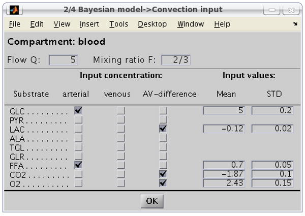
Convection input values. In this example, the user has specified some arterial and some arterio-venous differences in blood as input parameters.

Metabolica allows the user to reduce the model by assigning the values of some of the variables and to treat some of them as nuisance parameters or noise. In statistical terms, the former reduction corresponds to conditioning of the posterior density, the latter to marginalization. The model reduction is done via a dialog box like the one shown in Figure 6. The reduced components are selected by ticking on the buttons by the variables names, which in turns causes the opening of boxes where the mean and the standard deviation can be entered. If the used decides to fix a flux at a precise value, the STD is given as zero or N/A (default), otherwise, the variable is integrated out of the posterior density, and the mean and STD values are used as if the variable would be a fictitious measure corrupt by additive Gaussian noise with indicated standard deviation.

Figure 6.

Dialog box for model reduction. In the example, the user assumes a fictitious observed value for the decay flux of triacylglycerol to fatty acids and glycerol, with a given standard deviation, while the transport of fatty acyl-coenzyme A from cytosol to mitochondria is fixed.

Finally, the user is prompted to enter the prior information on the unknowns, namely the bounds to be obeyed by the unknowns and the parameters of the Gaussian portion of the prior, and measured values of the variables if available. An example of the dialog box used for this task is shown in Figure 7. Observe that the dialog box asks for upper and lower default bounds to avoid the distribution becoming indefinite, while for the Gaussian part, the default is N/A, indicating a missing piece of information.

Figure 7.

Dialog box for entering bounds, Gaussian priors and data. Observe that the three derivatives ticked by the user in the dialog box in Figure 4 are automatically added to the list of unknowns.

5.3 Exploration of the posterior and output analysis

The exploration of the posterior density requires the specification of the sample size and of the length of the burn-in period of the sample. If the sampling is initiated at a point of low posterior probability, it may require some time before the sampler arrives in the part of the parameter space with significant posterior probability. The initial part of the sample, referred to as the burn-in, is not representative for the posterior, and is usually discarded from the resulting sample. For more discussion, see, e.g., [20, 21, 27, 28]. The sample size and burn-in period are entered via the main dialog box shown in Figure 3.

Metabolica by default starts sampling from the midpoint of the interval defined by the bounds, but the user may specify a different starting point, obeying the bounds, which must be a variable in the Matlab workspace, whose name is entered in the Metabolica main dialog box.

The sampling algorithm used by Metabolica is the hybrid scheme described in Section 4. The test for the independence of sample is based on the normalized ACF and the IACT, in agreement with Section 4.3. Since the calculation of the ACF for large samples can be rather time consuming, the truncation index M_IMSE is estimated separately for each component. Moreover, the computation of the ACF is truncated at a value that lies within a user-specified interval, entered via the Metabolica main dialog box.

Having defined the specifics of the sampling, the user can point and click on the button Start sampling in the Metabolica main dialog box. The progress of the sampling can be monitored by a Matlab wait-bar that appears in a separate window.

After the sampling has been completed, a summary of the exploration of the posterior is presented as a list of the sample mean values, standard deviations and IACT values. The dialog box which displays the output in numerical form is shown in Figure 8. This window gives the user the option of a visual inspection of the sampling results.

Figure 8.

Output window for displaying the numerical results of the sampling. This window allows the user to select a graphical inspection of the results either as histograms or as pairwise scatter plots.

The histogram option plots sample histories, ACF, and histograms of selected individual components, as illustrated in Figure 9. In addition to inspecting the distributions of single components from the histogram plots, this window can also be used to judge whether the sample size is large enough and if the burn-in period was selected long enough. Sample histories of individual components which resemble “fuzzy worms” like those shown in Figure 9, together with ACF which decays to zero relatively fast are all indications that the sampler has explored well the posterior density.

Figure 9.

Visualization of the flux components as sample histories and histograms. The autocovariance function is plotted in the middle column.

The other graphical option available is the display of pairwise scatter plots of selected components. The output of this option is shown in Figure 10, with the histograms of individual components of the unknown vector on the diagonal. The user can select at maximum five unknowns at a time to be plotted pairwise in one window. Scatter plots can be very helpful at detecting functional dependencies between pairs of components of the vector of unknowns.

Figure 10.

Visualization of the sampling results using pairwise scatter plots of the components selected in the dialog window in Figure 8.

Finally, we point out that Metabolica offers the option of writing the full sample history in an ASCII file for further investigations.

6 Conclusion

The software package Metabolica comprises tools to construct and analyze complex metabolic network models within the Bayesian statistical framework. The current release of Metabolica contains the tools for building steady and stationary state models and performing Bayesian flux balance analysis, a Bayesian statistical analysis of the state of the system under steady or slowly changing conditions using MCMC sampling strategies. The current version of Metabolica is restricted to the use of Gaussian prior distributions with bounds. This limitation is not inherent to the methodology, but rather a choice of keeping the user interface as simple as possible. The sampling strategy of the package allows a modification to any parametric family of priors, although the SVD based coordinate transformation relies on the normality of the prior. Moreover, as the belief intervals themselves provided by the user may contain uncertainties, and additional layer based on hypermodels could be added to the analysis [21, 29]. These refinements add significantly to the complexity of the package and will be considered in later versions of the software.

Generally MCMC methods for large-scale problems are computationally burdensome. A common difficulty is slow convergence of the MCMC chain, even with sophisticated sampling algorithms. Slow convergence may be due to discrepancies in the model, conflicts between data and prior information or the presence of redundant variables. Numerous variations of the standard MCMC algorithms have been developed to improve the convergence of estimates and to reduce the burn-in, see, e.g., [30, 31]. The difficulty with the effective samplers is that they often require a good understanding how to tune the parameters if the sampler stalls, due, e.g., to bound constraints in high dimensions. The present MCMC algorithm in Metabolica requires no tuning by the user, and it is a compromise between user friendliness and efficiency. Model reduction may help in speeding up the convergence. Reductions of the model based on linear or affine constraints between the variables may be useful. These constraints may result by requiring some of the equations to be exactly satisfied from strong correlation between unknowns. The difficulty in including model reduction tools is that they should be compatible with the bound constraints, which may be difficult to check, see [5]. The implementation of model reduction via linear constraints will be included in a future release of Metabolica.

An extension of Metabolica suitable for dynamic studies within a statistical framework similar to that used for [1, 4, 7] is currently under development.

References

- 1.Calvetti D, Hageman R, Somersalo E. Large-scale Bayesian parameter estimation for a three compartment cardiac model during ischemia. Inverse Problems. 2006;22:1797–1817. [Google Scholar]
- 2.Calvetti D, Heino J, Somersalo E, Tunyan K. Bayesian stationary state flux balance analysis for a skeletal muscle metabolic model. Inverse Problems and Imaging. 2007;1:247–263. doi: 10.1016/j.jtbi.2007.04.002. [DOI] [PMC free article] [PubMed] [Google Scholar]
- 3.Calvetti D, Kuceyeski A, Somersalo E. Sampling-based analysis of a spatially distributed model for liver metabolism at steady state. Multiscale Modeling and Simulation. 2008;7:407–431. [Google Scholar]
- 4.Calvetti D, Somersalo E. Large-scale statistical parameter estimation in complex systems with an application to metabolic models. Multiscale Modeling and Simulation. 2006;5:1333–1366. [Google Scholar]
- 5.Heino J, Tunyan K, Calvetti D, Somersalo E. Bayesian flux balance analysis applied to skeletal muscle metabolic model. Journal of Theoretical Biology. 2007;248:91–110. doi: 10.1016/j.jtbi.2007.04.002. [DOI] [PMC free article] [PubMed] [Google Scholar]
- 6.Occhipinti R, Puchowicz M, LaManna JC, Somersalo E, Calvetti D. Statistical analysis of metabolic pathways of brain metabolism at steady state. Annals of Biomedical Engineering. 2007;6:886–902. doi: 10.1007/s10439-007-9270-5. [DOI] [PubMed] [Google Scholar]
- 7.Calvetti D, Somersalo E. Inverse problems and computational cell metabolic models: a statistical approach. Journal of Physics: Conference series. 2008;124:012003. [Google Scholar]
- 8.Hoops S, Sahle S, Gaues R, Lee C, Pahle J, Simus N, Singhal M, Xu L, Mendes P, Kummer U. COPASI – a COmplex PAthway SImulator. Bioinformatics. 2006;22:3067–3074. doi: 10.1093/bioinformatics/btl485. [DOI] [PubMed] [Google Scholar]
- 9.Klamt S, Saez-Rodrigues J, Gilles ED. Structural and functional analysis of celluer networks with CellNetAnalyzer. BMC Systems Biology. 2007;1(2) doi: 10.1186/1752-0509-1-2. [DOI] [PMC free article] [PubMed] [Google Scholar]
- 10.http://www.e-cell.org/
- 11.Becker SA, Feist AM, Mo ML, Hannum G, Palsson BO, Herrgard MJ. Quantitative prediction of cellular metabolism with constraint-based models: the COBRA Toolbox. Nature protocols. 2007;2:727–738. doi: 10.1038/nprot.2007.99. [DOI] [PubMed] [Google Scholar]
- 12.Schmidt H, Jirstrand M. Systems Biology Toolbox for MATLAB: a computational platform for research in systems biology. Bioinformatics. 2006;22:514–515. doi: 10.1093/bioinformatics/bti799. [DOI] [PubMed] [Google Scholar]
- 13.http://www.vcell.org/
- 14.Ramsey S, Orrell D, Bolouri H. Dizzy: stochastic simulation of large-scale genetic regulatory networks. J Bioinform Comput Biol. 2005;3:415–36. doi: 10.1142/s0219720005001132. [DOI] [PubMed] [Google Scholar]
- 15.Lunn DJ, Thomas A, Best N, Spiegelhalter D. WinBUGS – A Bayesian modelling framework: Concepts, structure, and extensibility. Statistics and Computing. 2000;10:325–337. [Google Scholar]
- 16.Bois FY. GNU MCSim: Bayesian statistical inference for SBML-coded systems biology models. Bioinformatics. 2009;25:1453–1454. doi: 10.1093/bioinformatics/btp162. [DOI] [PubMed] [Google Scholar]
- 17.Chalhoub E, Hanson R, Belovich J. A computer model of gluconeogenesis and lipid metabolism in the perfused liver. AJP - Endochrinol Metabolism. 2007;293:E1676–E1686. doi: 10.1152/ajpendo.00161.2007. [DOI] [PubMed] [Google Scholar]
- 18.Dash RK, Li Y, Kim J, Saidel GM, Cabrera ME. Modeling cellular metabolism and energetics in skeletal muscle: Large scale parameter estimation and sensitivity analysis. IEEE Tran Biomed Eng. 2008;55:1298–1318. doi: 10.1109/TBME.2007.913422. [DOI] [PubMed] [Google Scholar]
- 19.Zhou L, Stanley WC, Saidel GM, Yu X, Cabrera M. Regulation of lactate production at the onset of ischemia is independent of mitochondrial NADH/NAD+: insights from in silico studies. J Physiol. 2005 doi: 10.1113/jphysiol.2005.093146. 093146v1. [DOI] [PMC free article] [PubMed] [Google Scholar]
- 20.Kaipio J, Somersalo E. Statistical and Computational Inverse Problems. Springer; 2004. [Google Scholar]
- 21.Calvetti D, Somersalo E. Introduction to Bayesian Scientific Computing. Springer; 2007. [Google Scholar]
- 22.Schilling CH, Letcher D, Palsson BØ. Theory for the systemic definition of metabolic pathways and their use in interpreting metabolic function from a pathway-oriented perspective. J Teor Biol. 2000;203:229–248. doi: 10.1006/jtbi.2000.1073. [DOI] [PubMed] [Google Scholar]
- 23.Liu JS. Monte Carlo Strategies in Scientific Computing. Springer; 2003. [Google Scholar]
- 24.Geman S, Geman D. Stochastic relaxation, Gibbs distributions and Bayesian restoration of images. IEEE Trans Pattern Anal Mach Intell. 1984;6:721–741. doi: 10.1109/tpami.1984.4767596. [DOI] [PubMed] [Google Scholar]
- 25.Smith RL. Efficient Monte Carlo Procedures for generating points uniformly distributed over banded regions. Operations Res. 1984;32:1296–1308. [Google Scholar]
- 26.Geyer C. Practical Markov chain Monte Carlo. Statistical Science. 1992;7:473–511. [Google Scholar]
- 27.Gilks WR, Richardson S, Spiegelhalter D, editors. Markov Chain Monte Carlo in practice. Chapman & Hall/CRC; 1996. [Google Scholar]
- 28.Tan SM, Fox C, Nicholls GK. Lecture notes. Chapter 9 unpublished. http://www.math.auckland.ac.nz/
- 29.Bernardo JM, Smith AFM. Bayesian theory. J Wiley & Sons; 1993. [Google Scholar]
- 30.Tierney L, Mira A. Some adaptive Metropolis Hastings methods for Bayesian inference. Statistics in Medicine. 1999;18:2507–2515. doi: 10.1002/(sici)1097-0258(19990915/30)18:17/18<2507::aid-sim272>3.0.co;2-j. [DOI] [PubMed] [Google Scholar]
- 31.Haario H, Saksman E, Tamminen J. An adaptive Metropolis algorithm. Bernoulli. 1998;7:223–242. [Google Scholar]