A Comparison of Sample Size and Power in Case-Only Association Studies of Gene-Environment Interaction

Abstract

Assuming continuous, normally distributed environmental and categorical genotype variables, the authors compare 6 case-only designs for tests of association in gene-environment interaction. Novel tests modeling the environmental variable as either the response or the predictor and allowing a genetic variable with multiallelic variants are included. The authors show that tests imposing the same genotypic pattern of inheritance perform similarly regardless of whether genotype is the response variable or the predictor variable. The novel tests using the genetic variable as the response variable are advantageous because they are robust to non-normally distributed environmental exposures. Dominance deviance—deviation from additivity in the main or interaction effects—is key to test performance: When it is zero or modest, tests searching for a trend with increasing risk alleles are optimal; when it is large, tests for genotypic effects are optimal. However, the authors show that dominance deviance is attenuated when it is observed at a proxy locus, which is common in genome-wide association studies, so large dominance deviance is likely to be rare. The authors conclude that the trend test is the appropriate tool for large-scale association scans where the true gene-environment interaction model is unknown. The common practice of assuming a dominant pattern of inheritance can cause serious losses of power in the presence of any recessive, or modest dominant, effects.

Gene-environment (G-E) interaction refers to variation in the effect of genetic factors, measured in a suitable scale, as a function of variation in environmental exposure and vice versa. Case-only study designs have been shown to be more powerful than case-control study designs in the assessment of possible interactions between genetic factors and environmental exposures in the etiology of a disease (1, 2). The ability to test for G-E interaction using the case population only may be advantageous—for example, in studies that rely on public population control data for which information on environmental exposures of interest is not available. Assuming independence between environment and genotype in the population of controls, Begg and Zhang (3), Piegorsch et al. (2), Umbach and Weinberg (4), and Yang et al. (5) showed that efficient estimates of interaction for categorical environment and binary genotype variables can be obtained via logistic regression in a case-only analysis. Albert et al. (6), Armstrong (7), and Cheng (8) explored extensions to continuous environment and categorical genotype variables using both logistic and multinomial regression. Typically, the genetic factor is treated as the response variable, with the environmental exposure being used as the predictor variable; the converse, whereby the response variable is the environmental exposure and thus the effect of a genetic factor on the association between the environmental exposure and disease is studied, has received less attention. With the genetic factor used as the predictor variable rather than the response variable, there is greater freedom to categorize it appropriately. By definition, a successful finding in either situation represents a G-E interaction. Kraft et al. (9) compared the power and sample-size requirements of various case-control study designs for testing for G-E interaction to a single case-only design that assumed a dominant inheritance pattern at the genetic locus. Like other investigators (2, 5), Kraft et al. showed that in the presence of any interaction effect, the case-only design was most powerful.

Here we consider a categorical genetic variable G and a normally distributed environmental exposure variable E. We assume independence between G and E in the population under study and compare the power and sample-size requirements of 6 case-only tests for detecting G-E interaction. Three categorizations of G are considered: binary, ordinal, and nominal. The first 3 tests model E as the response variable using a linear regression with each category of G as the predictor. The remaining 3 tests use multinomial regression techniques to allow each categorization of G to be the response variable, with E as the predictor variable: A logistic regression (this test is the same as that examined by Kraft et al. (9)), a proportional odds regression, and a multinomial regression are performed for binary, ordinal, and nominal codings of G. Each test is considered under 3 different penetrance models that are based on logistic risk models.

MATERIALS AND METHODS

Models

Let D be an indicator of disease (D = 1 if affected and D = 0 otherwise), E a standard normally distributed environmental exposure variable, and g a genotype at a disease susceptibility locus G with alleles A and a. Let p_A denote the prevalence of the minor allele, A. Let G denote the minor allele count: G = 0 when g = a/a, G = 1 when g = a/A, and G = 2 when g = A/A. Let G_D equal 1 when g = a/A; otherwise, G_D = 0. G is then an additive genotype coding and G_D is its deviation from additivity.

We consider true penetrance models based on the log odds of disease:

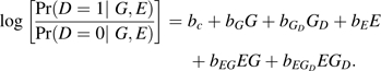(1)

b_G represents an additive genetic main effect with b_GD its deviation from additivity, hereafter referred to as dominance deviance; b_E represents an environmental main effect; and b_EG represents an additive G-E interaction effect with b_EGD its dominance deviance. In practical terms, b_E represents the log odds ratio for disease risk associated with a 1-unit increase in E among persons with no minor alleles; b_G + b_GD and 2b_G are the log odds ratios associated with an increase of 1 and 2 minor alleles, respectively, in persons with zero exposure, etc. We assume that G and E are independent in the population under study.

Cases are persons affected by the disease of interest (D = 1). Below we describe the 6 case-only tests considered. Each test is based on a model that generates a log likelihood, and tests of G-E interaction are based on standard likelihood ratio statistics. The specific likelihoods associated with each model and our approach to power and sample-size estimation are described in the Web Appendix, which is posted on the Journal’s Web site (http://aje.oxfordjournals.org/).

Linear regression additive (EG_T) model.

The relation between E and G is modeled as a simple linear regression assuming additive genetic effects at the genetic locus:

The likelihood ratio test constrains β_EG⁽¹⁾≡0 under the null hypothesis and has 1 df. This test assumes a trend in risk with an increasing number of risk alleles and is referred to as a trend test.

Linear regression dominant (EG_D) model.

The relation between E and G is modeled as a simple linear regression, assuming a dominant pattern of inheritance at the genetic locus: G_DOM = 1 for carriers of the minor allele and zero otherwise.

The likelihood ratio test constrains β_EGDOM⁽²⁾≡0 under the null hypothesis and has 1 df. This test is referred to as a dominant test.

Linear regression deviation additivity (EG_G) model.

The relation between E and G is modeled as a simple linear regression but with the introduction of a term to model any dominance deviance associated with the interaction:

The likelihood ratio test constrains β_EG⁽³⁾≡0 and β_EGD⁽³⁾≡0 under the null hypothesis and has 2 df. This test allows independent genotype effects and is referred to as a genotypic test.

Logistic regression dominant (G_DE) model.

The relation between carriers of the minor allele and E is modeled as a logistic regression:

If the genetic factor and the environmental exposure are independent among the cases, then β_EG⁽⁴⁾ is a consistent estimator of the interaction parameter measuring the departure of the joint effects of E and G_DOM from multiplicative risk ratios (8). If the disease is rare, then β_EG⁽⁴⁾ is also a good estimator of the interaction parameter measuring the departure of the joint effects of E and G_DOM from multiplicative odds ratios. The likelihood ratio test constrains β_EG⁽⁴⁾≡0 under the null hypothesis of no interaction and has 1 df. Like EG_D, this test assumes a dominant pattern of inheritance at the genetic locus and is referred to as a dominant test.

Proportional odds regression (G_TE) model.

We compare the probability of an equal or smaller number of high-risk alleles, G ≤ k, to the probability of a larger number, G > k, as a function of the continuous environmental exposure E:

If β_EG⁽⁵⁾ > 0, then increasing values of E are associated with increasing genetic risk in the case population. The likelihood ratio test constrainsβ_EG⁽⁵⁾≡0 under the null hypothesis of no interaction and has 1 df. Like EG_T, this test assumes a trend in risk with an increasing number of risk alleles and is referred to as a trend test.

Multinomial regression genetic response (G_GE) model.

The probability of observing 1 or 2 minor alleles is compared with the probability of observing none:

The likelihood ratio test constrainsβ_EG1⁽⁶⁾≡0 and β_EG2⁽⁶⁾≡0 under the null hypothesis and has 2 df. Like EG_G, this test allows independent genotype risks and is referred to as a genotypic test.

Power calculations

We calculated the number of cases required to achieve 80% statistical power, as well as the power for 1,000 case participants, to detect G-E interaction at the disease susceptibility locus G. We considered a range of minor allele frequencies (p_A = 0.1, 0.25), genetic main effects (b_G = 0, log(1.3)), environmental main effects (b_E = 0, log(1.3)), and G-E interaction effects (b_EG = 0, log(1.1), log(1.2), log(1.3)). To reduce the dimensionality of the model parameter space, we assumed a common value δ for the dominance deviance associated with main and interaction genetic effects: δ = b_GD = b_EGD. When δ = 0, the model is additive and when δ > 0 (respectively, δ < 0), dominant (respectively, recessive) main and interaction genetic effects are present in the underlying model. We considered a range of realistic disease models by allowing the dominance deviance to vary within the range ± min(b_G,b_EG) to ensure no heterozygote advantage: If δ > b_EG, for example, then the penetrance associated with the heterozygotic genotype may be greater than the homozygotic genotype giving a heterozygote advantage.

We also performed similar calculations assuming that the interaction was observed at a nearby noncausal locus H with minor allele frequency p_B = 0.2 and the maximum value of linkage disequilibrium r² between alleles at the disease susceptibility locus G. There are algebraic restrictions on the range of r² (10), and the maximum value of linkage disequilibrium between alleles at G and H when p_B = 0.2 depends on the value of p_A: When p_A = 0.1, maximum r² = 0.44; when p_A = 0.25, maximum r² = 0.75; and when p_A = 0.4, maximum r² = 0.37. All tests assumed a 2-sided alternative hypothesis and a significance level of 0.05.

One of the underlying assumptions of the tests of interaction with E as the response, EG_T, EG_D, and EG_G, is that E is normally distributed. In order to assess the effect of nonnormality of E, we calculated power when only cases with extreme values of E, |E| > 1, were included and when 10% of cases were allowed to have extreme values of E with 9 times the standard deviation of the remaining 90% of cases.

Example: study of G-E interaction for lung cancer

In a case-control study, Zhou et al. (11) found an interaction between polymorphisms in the excision repair cross-complementing group 2 (ERCC2) gene and cumulative cigarette smoking exposure in lung cancer. They studied 1,092 cases and 1,240 controls selected from the same Caucasian population. Using parameter values estimated from their analyses and a true penetrance model of the form given in equation 1, we calculated the number of samples that would be required to achieve 80% power in a standard case-control test of G-E interaction, as well as in our 6 case-only tests.

RESULTS

General design comparisons

The number of cases required to achieve 80% power in each of the dominant tests, G_DE and EG_D, hardly differs for any set of parameter values studied (Tables 1, 2, and 3). Similarly, approximately equivalent numbers of cases are also required to achieve the same power in the genotypic tests, EG_G and G_GE, with the largest differences being seen at the largest main interaction effect sizes. The trend tests EG_T and G_TE require similar numbers of cases to achieve the same power under a strictly additive model but show greater differences in the presence of any dominance deviance.

Table 1.

Sampling Units for Case-Only Tests of Gene-Environment Interaction at a Disease Susceptibility Locus G Under Zero Deviation from Additivity^a

pA	ebG	ebE	ebEG	Additive δ = 0
				EGT	EGD	EGG	GDE	GTE	GGE
0.1	1	1	1.1	4,793	1.1	1.2	1.1	1	1.2
0.1	1	1	1.2	1,292	1.1	1.2	1.1	1	1.2
0.1	1	1	1.3	611	1.1	1.2	1.1	1	1.2
0.1	1	1.3	1.1	4,699	1.1	1.2	1.1	1	1.2
0.1	1	1.3	1.2	1,244	1.1	1.2	1.1	1	1.2
0.1	1	1.3	1.3	579	1.1	1.2	1.1	1	1.2
0.1	1.3	1	1.1	3,912	1.1	1.2	1.1	1	1.2
0.1	1.3	1	1.2	1,054	1.1	1.2	1.1	1	1.2
0.1	1.3	1	1.3	499	1.1	1.2	1.1	1	1.2
0.1	1.3	1.3	1.1	3,841	1.1	1.2	1.1	1	1.2
0.1	1.3	1.3	1.2	1,018	1.1	1.2	1.1	1	1.2
0.1	1.3	1.3	1.3	474	1.1	1.2	1.1	1	1.2
0.25	1	1	1.1	2,301	1.2	1.2	1.2	1	1.2
0.25	1	1	1.2	621	1.2	1.2	1.2	1	1.2
0.25	1	1	1.3	294	1.2	1.2	1.2	1	1.2
0.25	1	1.3	1.1	2,273	1.2	1.2	1.2	1	1.2
0.25	1	1.3	1.2	606	1.2	1.2	1.2	1	1.2
0.25	1	1.3	1.3	285	1.2	1.2	1.2	1	1.2
0.25	1.3	1	1.1	2,046	1.2	1.2	1.2	1	1.2
0.25	1.3	1	1.2	553	1.2	1.2	1.2	1	1.2
0.25	1.3	1	1.3	262	1.2	1.2	1.2	1	1.2
0.25	1.3	1.3	1.1	2,027	1.2	1.2	1.2	1	1.2
0.25	1.3	1.3	1.2	543	1.2	1.2	1.2	1	1.2
0.25	1.3	1.3	1.3	256	1.3	1.2	1.3	1	1.2
0.4	1	1	1.1	1,800	1.3	1.2	1.3	1	1.2
0.4	1	1	1.2	487	1.3	1.2	1.4	1	1.2
0.4	1	1	1.3	232	1.4	1.2	1.4	1	1.2
0.4	1	1.3	1.1	1,792	1.3	1.2	1.3	1	1.2
0.4	1	1.3	1.2	483	1.4	1.2	1.4	1	1.2
0.4	1	1.3	1.3	230	1.4	1.2	1.4	1	1.2
0.4	1.3	1	1.1	1,739	1.4	1.2	1.4	1	1.2
0.4	1.3	1	1.2	472	1.5	1.2	1.5	1	1.2
0.4	1.3	1	1.3	226	1.5	1.2	1.5	1	1.2
0.4	1.3	1.3	1.1	1,737	1.4	1.2	1.4	1	1.2
0.4	1.3	1.3	1.2	471	1.5	1.2	1.5	1	1.2
0.4	1.3	1.3	1.3	226	1.5	1.2	1.5	1	1.2

^aNumber of sampling units required for case-only test of gene-environment interaction EG_T to achieve 80% power for a range of environmental and genetic main effects and gene-environment interaction effects under zero dominance deviance and the ratio of sampling units required in each of the other tests to achieve the same power in comparison with the number required in EG_T. Dominance deviance is defined as the deviation from additivity in the main or interaction effects: Here we assume that the dominance deviance in the main effect and the interaction effect are the same. A sampling unit is a case.

Table 2.

Sampling Units for Case-Only Tests of Gene-Environment Interaction at a Disease Susceptibility Locus G Under Positive Deviation from Additivity^a

pA	ebG	ebE	ebEG	Positive Deviation from Additivity (δ > 0 [δ = log(1.1)])
				EGT	EGD	EGG	GDE	GTE	GGE
0.1	1	1	1.1	1,390	0.9	1.2	0.9	1	1.2
0.1	1	1	1.2	607	1	1.2	1	1	1.2
0.1	1	1	1.3	348	1	1.2	1	1	1.2
0.1	1	1.3	1.1	1,351	0.9	1.2	0.9	1	1.2
0.1	1	1.3	1.2	582	1	1.2	1	1	1.2
0.1	1	1.3	1.3	330	1	1.2	1	1	1.2
0.1	1.3	1	1.1	1,217	0.9	1.2	0.9	0.9	1.1
0.1	1.3	1	1.2	522	1	1.2	1	1	1.2
0.1	1.3	1	1.3	298	1	1.2	1	1	1.2
0.1	1.3	1.3	1.1	1,189	0.9	1.2	0.9	0.9	1.1
0.1	1.3	1.3	1.2	505	1	1.2	1	1	1.2
0.1	1.3	1.3	1.3	284	1	1.2	1	1	1.2
0.25	1	1	1.1	1,019	0.9	1.1	0.9	0.9	1.1
0.25	1	1	1.2	396	1	1.2	1	0.9	1.2
0.25	1	1	1.3	217	1	1.2	1	1	1.2
0.25	1	1.3	1.1	1,019	0.9	1.1	0.9	0.9	1
0.25	1	1.3	1.2	395	1	1.1	1	0.9	1.2
0.25	1	1.3	1.3	215	1	1.2	1	1	1.2
0.25	1.3	1	1.1	1,065	0.8	1	0.8	0.9	1
0.25	1.3	1	1.2	393	0.9	1.1	1	0.9	1.1
0.25	1.3	1	1.3	211	1	1.2	1	1	1.2
0.25	1.3	1.3	1.1	1,076	0.8	1	0.8	0.9	1
0.25	1.3	1.3	1.2	396	0.9	1.1	1	0.9	1.1
0.25	1.3	1.3	1.3	212	1	1.2	1	1	1.2
0.4	1	1	1.1	1,305	0.7	0.9	0.7	0.9	0.9
0.4	1	1	1.2	425	0.9	1.1	0.9	1	1.1
0.4	1	1	1.3	218	1	1.2	1.1	1	1.2
0.4	1	1.3	1.1	1,338	0.7	0.9	0.7	0.9	0.9
0.4	1	1.3	1.2	437	0.9	1.1	0.9	1	1.1
0.4	1	1.3	1.3	224	1	1.2	1.1	1	1.2
0.4	1.3	1	1.1	1,607	0.7	0.8	0.7	1	0.8
0.4	1.3	1	1.2	473	0.9	1.1	0.9	1	1.1
0.4	1.3	1	1.3	234	1.1	1.2	1.1	1	1.2
0.4	1.3	1.3	1.1	1,665	0.7	0.8	0.7	1	0.8
0.4	1.3	1.3	1.2	491	0.9	1.1	0.9	1	1.1
0.4	1.3	1.3	1.3	244	1.1	1.1	1.1	1	1.2

^aNumber of sampling units required for case-only test of gene-environment interaction EG_T to achieve 80% power for a range of environmental and genetic main effects and gene-environment interaction effects under positive dominance deviance and the ratio of sampling units required in each of the other tests to achieve the same power in comparison with the number required in EG_T. Dominance deviance is defined as the deviation from additivity in the main or interaction effects: Here we assume that the dominance deviance in the main effect and the interaction effect are the same. A sampling unit is a case.

Table 3.

Sampling Units for Case-Only Tests of Gene-Environment Interaction at a Disease Susceptibility Locus G Under Negative Deviation from Additivity^a

pA	ebG	ebE	ebEG	Negative Deviation from Additivity (δ < 0 [δ = − log(1.1)])
				EGT	EGD	EGG	GDE	GTE	GGE
0.1	1	1	1.1	106,376	4.1	0.2	4.1	2.8	0.2
0.1	1	1	1.2	3,835	1.3	1.1	1.3	1.2	1.1
0.1	1	1	1.3	1,233	1.2	1.2	1.2	1.1	1.2
0.1	1	1.3	1.1	97,376	4.1	0.3	4	2.8	0.3
0.1	1	1.3	1.2	3,638	1.3	1.1	1.3	1.2	1.1
0.1	1	1.3	1.3	1,154	1.2	1.2	1.2	1.1	1.2
0.1	1.3	1	1.1	54,648	4.1	0.3	4.1	2.6	0.3
0.1	1.3	1	1.2	2,804	1.4	1.1	1.4	1.2	1.1
0.1	1.3	1	1.3	936	1.3	1.2	1.3	1.2	1.2
0.1	1.3	1.3	1.1	50,221	4.1	0.3	4.1	2.6	0.3
0.1	1.3	1.3	1.2	2,651	1.4	1.1	1.4	1.3	1
0.1	1.3	1.3	1.3	874	1.3	1.2	1.3	1.2	1.2
0.25	1	1	1.1	8,318	4.3	0.5	4.3	1.7	0.5
0.25	1	1	1.2	1,068	1.7	1	1.7	1.2	1
0.25	1	1	1.3	412	1.5	1.1	1.5	1.2	1.2
0.25	1	1.3	1.1	7,758	4.3	0.5	4.3	1.7	0.5
0.25	1	1.3	1.2	1,005	1.8	1	1.8	1.2	1
0.25	1	1.3	1.3	385	1.5	1.2	1.5	1.2	1.2
0.25	1.3	1	1.1	5,099	4.5	0.6	4.5	1.5	0.6
0.25	1.3	1	1.2	817	1.9	1.1	1.9	1.2	1
0.25	1.3	1	1.3	331	1.6	1.1	1.6	1.1	1.2
0.25	1.3	1.3	1.1	4,791	4.4	0.6	4.4	1.5	0.6
0.25	1.3	1.3	1.2	771	1.9	1.1	1.9	1.2	1.1
0.25	1.3	1.3	1.3	311	1.7	1.2	1.7	1.1	1.2
0.4	1	1	1.1	2,607	4.8	0.7	4.8	1.2	0.7
0.4	1	1	1.2	563	2.2	1.1	2.2	1.1	1.1
0.4	1	1	1.3	248	1.9	1.2	1.9	1.1	1.2
0.4	1	1.3	1.1	2,482	4.7	0.7	4.7	1.2	0.7
0.4	1	1.3	1.2	537	2.2	1.1	2.2	1.1	1.1
0.4	1	1.3	1.3	237	1.9	1.2	1.9	1.1	1.2
0.4	1.3	1	1.1	1,894	5.1	0.8	5.1	1	0.8
0.4	1.3	1	1.2	475	2.5	1.1	2.5	1	1.1
0.4	1.3	1	1.3	220	2.1	1.2	2.1	1	1.2
0.4	1.3	1.3	1.1	1,821	5	0.8	5	1	0.8
0.4	1.3	1.3	1.2	457	2.5	1.1	2.5	1	1.1
0.4	1.3	1.3	1.3	212	2.1	1.2	2.1	1	1.2

^aNumber of sampling units required for case-only test of gene-environment interaction EG_T to achieve 80% power for a range of environmental and genetic main effects and gene-environment interaction effects under negative dominance deviance and the ratio of sampling units required in each of the other tests to achieve the same power in comparison with the number required in EG_T. Dominance deviance is defined as the deviation from additivity in the main or interaction effects: Here we assume that the dominance deviance in the main effect and the interaction effect are the same. A sampling unit is a case.

Figure 1 shows the power of the tests to detect G-E interaction with 1,000 case participants as a function of the dominance deviance when observing genotypes at a disease susceptibility locus. Under the null hypothesis, when there is no G-E interaction present in the underlying model (b_EG = 0 and δ = 0), none of the tests show any increase in the false-positive rate; that is, they all have power equal to the type I error rate. In the presence of no dominance deviance or a slight dominance deviance, δ≈0, the trend tests are the most powerful. For example, Figure 1, part D, shows that the trend tests are most powerful for dominance deviance in the range −0.06 < δ < 0.05. While the strictly additive trend test EG_T appears to be marginally preferable compared with the proportional odds trend test G_TE, there is little information with which to choose between the 2 tests at low values of dominance deviance.

Figure 1.

Statistical power to detect gene-environment interaction for 1,000 case participants as a function of the dominance deviance δ for tests EG_T (solid lines), EG_D (dashed lines), EG_G (dotted lines), and G_TE (dashed-dotted lines) at a disease susceptibility locus G for various values of the high-risk allele frequency p_A and interaction effect size b_EG: A) p_A = 0.1, b_EG = log(1.1); B) p_A = 0.1, b_EG = log(1.2); C) p_A = 0.1, b_EG = log(1.3); D) p_A = 0.25, b_EG = log(1.1); E) p_A = 0.25, b_EG = log(1.2); F) p_A = 0.25, b_EG = log(1.3). Dominance deviance is defined as the deviation from additivity in the main or interaction effects: Here we assume that the dominance deviance in the main effect and the interaction effect are the same. Results are shown for the situation where there is no main environmental effect, b_E = 0, and the main genetic effect is b_G = log(1.3); variation in the sizes of main environmental or genetic effects resulted in only minor variations in power and not did not alter conclusions regarding the relative efficacies of the tests considered. The environmental exposure variable was normally distributed and standardized.

For larger positive dominance deviance, δ >> 0, indicating large dominant effects, the dominant tests are, as expected, most powerful. However, for any negative dominance deviance, δ < 0, suggesting a tendency towards recessive effects at the genetic locus, the dominant tests perform poorly in comparison with other tests. The genotypic tests are only optimal in the presence of large absolute values of δ: When large and dominant (δ >> 0), they equal the dominant tests, and when large and recessive (δ << 0), they outshine all of the other tests.

But how likely is a large dominance deviance? When testing at a noncausal locus with alleles that are not in complete linkage disequilibrium with alleles at the causal locus (r² < 1), common in genome-wide association studies, the observed effects are attenuated; in particular, the apparent dominance deviance at the noncausal locus is reduced in comparison with that observed at the causal locus (see Web Appendix (http://aje.oxfordjournals.org/) for discussion). Thus, the chance of a large dominance deviance is even less when testing at a noncausal locus, suggesting that use of genotypic tests must be carefully considered and that the comparison between tests in the presence of low dominance deviance is of the greatest practical importance. Figure 2 shows the power of the tests to detect G-E interaction with 1,000 case participants as a function of the dominance deviance when observing genotypes at a noncausal locus in linkage disequilibrium with the disease susceptibility locus described in Figure 1. While power, in general, is lower when testing at a noncausal locus, a comparison of Figures 1 and 2 indicates that the same pattern of test efficacy according to variation in δ holds when testing at a noncausal locus as when testing at the disease susceptibility locus, except that the range of values of δ for which the trend tests are optimal is wider.

Figure 2.

Statistical power to detect gene-environment interaction for 1,000 case participants as a function of the dominance deviance δ for tests EG_T (solid lines), EG_D (dashed lines), EG_G (dotted lines), and G_TE (dashed-dotted lines) at a noncausal locus H with minor allele frequency p_B = 0.2 for various values of the minor allele frequency p_A and interaction effect size b_EG at the disease susceptibility locus G: A) p_A = 0.1, b_EG = log(1.1); B) p_A = 0.1, b_EG = log(1.2); C) p_A = 0.1, b_EG = log(1.3); D) p_A = 0.25, b_EG = log(1.1); E) p_A = 0.25, b_EG = log(1.2); F) p_A = 0.25, b_EG = log(1.3). The alleles at H are in maximum linkage disequilibrium (r²) with the alleles at G: when p_A = 0.1, r² = 0.44; when p_A = 0.25, r² = 0.75; and when p_A = 0.4, r² = 0.37. Dominance deviance is defined as the deviation from additivity in the main or interaction effects: Here we assume that the dominance deviance in the main effect and the interaction effect are the same. Results are shown for the situation where there is no main environmental effect, b_E = 0, and the main genetic effect is b_G = log(1.3); variation in the sizes of main environmental or genetic effects resulted in only minor variations in power and not did not alter conclusions regarding the relative efficacies of the tests considered. The environmental exposure variable was normally distributed and standardized.

When cases were selectively sampled so that only those with extreme values of E, |E| > 1, were included, the power of all tests was increased, but there were no changes in conclusions regarding relative test efficacies (results not shown). This increase in power under selective sampling was previously observed by Boks et al. (12). Furthermore, under this modest nonnormality, there was no increase in the false-positive error rate in any of the tests when no G-E interaction was present in the underlying model. When more extreme departure from normality was allowed, so that 10% of cases were allowed to have environmental exposure values with standard deviations 9 times that of the remaining 90% of cases, the type I error rate for the tests with E as the response variable did increase, but only marginally—for example, from 0.05 to an average of 0.0507 in EG_T. Results suggest that the tests EG_T, EG_D, and EG_G, where E is assumed to be a normally distributed response, are robust to this type of nonnormality.

Example: study of G-E interaction for lung cancer

Zhou et al. (11) considered a standard case-control test of G-E interaction between the ERCC2 polymorphism Asp312Asn and the square root of pack-years of smoking which adjusted for age, sex, smoking status, time since smoking cessation (years), and the interaction between smoking status and the square root of pack-years. The frequency of the Asp allele (Asp312Asn) was 0.3, the square root of pack-years was approximately normally distributed with mean and standard deviation 3, and the adjusted odds ratios for lung cancer risk in persons with zero pack-years were 1.5 (95% confidence interval: 1.0, 2.3) for the Asp/Asn genotype and 3.4 (95% confidence interval: 1.9, 6.0) for the Asn/Asn genotype (when each was compared with the Asp/Asp genotype). These risks decreased by exp(−0.07√k) for the heterozygous Asp/Asn genotype and by exp(−0.17√k) for the homozygous Asn/Asn genotype for k pack-years. The decrease in risk was not significant for the homozygous genotype and was only significant up to approximately 30 pack-years for the heterozygous genotype. Further analysis of Zhou et al.’s results suggests that the unadjusted odds ratio for lung cancer risk in persons with the Asp/Asp genotype associated with k pack-years of smoking was in the approximate range exp(0.3√k) to exp(0.4√k).

Assuming these parameter values, Table 4 compares the numbers of samples required to achieve 80% power in a standard case-control test of G-E interaction, as well as in our 6 case-only tests. Our results are unadjusted for any other covariates. The case-only tests require substantially fewer sampling units than the case-control tests. The most powerful test is EG_T, closely followed by G_TE. These tests both search for a trend in the interaction with increasing number of risk alleles. The model virtually stipulates zero dominance deviance associated with the interaction effect (b_EGD = 0.01), indicating that the extra degree of freedom required by using EG_G and G_GE rather than EG_T or G_TE is not warranted. However, the estimated dominance deviance for the main genetic effect is negative (b_GD = − 0.22), suggesting a slight recessive effect and making it much more difficult for the tests imposing a dominant model on the genotype, EG_D and G_DE, to detect effects. Notice that the marginal effect size of pack-years on lung cancer risk does not alter conclusions regarding the relative test efficacies.

Table 4.

Numbers of Sampling Units Required to Achieve 80% Power to Detect a Gene-Environment Interaction Between the ERCC2 Asp312Asn Polymorphism and Pack-Years of Smoking^a

bE	Case-Control Test	Case-Only Tests
		EGT	EGD	EGG	GDE	GTE	GGE
0.25	1,059	238	325	291	329	252	295
0.30	1,151	244	331	298	335	259	303
0.35	1,271	252	340	308	344	268	312
0.40	1,424	264	354	321	358	281	326
0.45	1,614	282	380	343	384	303	348
0.60	1,847	314	428	381	432	340	387

Abbreviation: ERCC2, excision repair cross-complementing group 2.

^aThe true penetrance model is of the form given in equation 1 (see text), and effect sizes are b_G = 0.61, b_GD = − 0.22, b_EG = − 0.09, and b_EGD = 0.01, as estimated by Zhou et al. (11). Results are shown for values of b_E as indicated for a 2-df case-control test of G-E interaction and our 6 case-only tests of G-E interaction. A sampling unit is a pair for the case-control test and a case for the case-only tests.

DISCUSSION

We compared the power and sample-size requirements of 6 case-only tests for detecting interaction between a genetic factor and a continuous environmental exposure in association with disease. Under the null hypothesis of no G-E interaction, none of the tests showed any increase in the false-positive rate, while under the complementary hypothesis, all of the tests had power greater than the type I error rate. We conclude that these tests are valid tests of G-E interaction. More work will be required to interpret the estimated coefficients from these case-only regressions in terms of risk ratios and other measures of effect size.

In order to simplify analyses, a commonly used approach in case-only tests of G-E interaction is to assume either an autosomal dominant or recessive inheritance pattern at the genetic locus (8, 9, 13, 14). Such models are represented in the tests G_DE and EG_D. The novel tests based on multinomial and proportional odds models that we considered here allow for alternative patterns of genetic inheritance.

For normally distributed environmental exposures, we have shown that EG_D, a test using linear regression with the environmental variable as the response variable, requires similar numbers of cases as G_DE, a test using logistic regression with the genetic variable as the response variable, in order to achieve the same power. Similarly, EG_G and G_GE also require similar numbers of cases to achieve equivalent power. This is as expected, since these pairs of tests each model the genetic variable in the same manner; the genetic variant is modeled as dominant in G_DE and EG_D and as genotypic in EG_G and G_GE. Whereas EG_T imposes an additive model on the genetic variable, G_TE only imposes a trend in the form of its proportional odds assumption. As such, these 2 “trend” tests show greater differences between the numbers of cases required to achieve the same power in any given scenario.

EG_T, EG_D, and EG_G depend on an assumption that the environmental exposure is normally distributed, and while we have shown that departure from normality need not have a significant impact on power outcomes, G_DE, G_TE, and G_GE are clearly advantageous, since they do not require this assumption and are robust to non-normally distributed environmental exposures (15). Careful consideration of the scale of measurement is important, because changing the scale, such as transforming a quantitative environmental variable, can remove or add G-E interaction.

We have shown that the dominance deviance is key to determining the optimal test. For zero (suggesting strictly additive genetic effects) or modest (suggesting slight recessive or dominant genetic effects) dominance deviance, the trend tests, EG_T and G_TE, are optimal. For large positive dominance deviance (suggesting a large dominant genetic effect), the dominant tests EG_D and G_DE are strictly optimal, closely followed by the genotypic tests EG_G and G_GE. However, if the dominance deviance is actually negative (suggesting a recessive genetic effect), the choice of a dominant test can have severe implications for power, and in the presence of a large recessive genetic effect, only a genotypic test will be suitable. Hence, if the dominance deviance is large but of unknown direction, the genotypic test is the safest choice. However, we showed that when testing at a noncausal locus, the dominance deviance at the observed locus is attenuated. Thus, for the genotypic tests to outperform the trend tests, dominance deviance at the disease susceptibility locus must be very large when testing for G-E interaction at a noncausal locus with alleles in less-than-perfect linkage disequilibrium with alleles at the causal locus. We conclude that the trend test is the most robust choice for large-scale association scans where the true G-E interaction model is unknown. The common practice of assuming a dominant pattern of inheritance can cause serious losses of power in the presence of any recessive, or modest dominant, effects.

The exemplary data method used to calculate power relies on asymptotic distributions, and the results presented here are valid for the large sample sizes typically seen in current association studies. In critical applications, simulation studies would be required to determine precise power estimates (16).

The case-only tests presented here are only valid under the assumption of independence between gene and environmental variables; any dependence between these variables will be reflected in the case series even in the absence of G-E interaction and will lead to biased estimates of interaction. Independence is therefore required to protect against false-positive findings. Empirical studies have suggested that violation of gene-environment independence, when it occurs, is usually modest (17), but more work will be required to categorize the impact of departure from gene-environment independence on the relative efficacies of the tests considered here.

Glossary

Abbreviations

ERCC2

excision repair cross-complementing group 2

G-E

gene-environment

References

- 1.Khoury MJ, Flanders WD. Nontraditional epidemiologic approaches in the analysis of gene-environment interaction: case-control studies with no controls! Am J Epidemiol. 1996;144(3):207–213. doi: 10.1093/oxfordjournals.aje.a008915. [DOI] [PubMed] [Google Scholar]
- 2.Piegorsch WW, Weinberg CR, Taylor JA. Non-hierarchical logistic models and case-only designs for assessing susceptibility in population-based case-control studies. Stat Med. 1994;13(2):153–162. doi: 10.1002/sim.4780130206. [DOI] [PubMed] [Google Scholar]
- 3.Begg CB, Zhang ZF. Statistical analysis of molecular epidemiology studies employing case-series. Cancer Epidemiol Biomarkers Prev. 1994;3(2):173–175. [PubMed] [Google Scholar]
- 4.Umbach DM, Weinberg CR. Designing and analysing case-control studies to exploit independence of genotype and exposure. Stat Med. 1997;16(15):1731–1743. doi: 10.1002/(sici)1097-0258(19970815)16:15<1731::aid-sim595>3.0.co;2-s. [DOI] [PubMed] [Google Scholar]
- 5.Yang Q, Khoury MJ, Flanders WD. Sample size requirements in case-only designs to detect gene-environment interaction. Am J Epidemiol. 1997;146(9):713–720. doi: 10.1093/oxfordjournals.aje.a009346. [DOI] [PubMed] [Google Scholar]
- 6.Albert PS, Ratnasinghe D, Tangrea J, et al. Limitations of the case-only design for identifying gene-environment interactions. Am J Epidemiol. 2001;154(8):687–693. doi: 10.1093/aje/154.8.687. [DOI] [PubMed] [Google Scholar]
- 7.Armstrong BG. Fixed factors that modify the effects of time-varying factors: applying the case-only approach. Epidemiology. 2003;14(4):467–472. doi: 10.1097/01.ede.0000071408.39011.99. [DOI] [PubMed] [Google Scholar]
- 8.Cheng KF. A maximum likelihood method for studying gene-environment interactions under conditional independence of genotype and exposure. Stat Med. 2006;25(18):3093–3109. doi: 10.1002/sim.2506. [DOI] [PubMed] [Google Scholar]
- 9.Kraft P, Yen YC, Stram DO, et al. Exploiting gene-environment interaction to detect genetic associations. Hum Hered. 2007;63(2):111–119. doi: 10.1159/000099183. [DOI] [PubMed] [Google Scholar]
- 10.Weir BS. Inferences about linkage disequilibrium. Biometrics. 1979;35(1):235–254. [PubMed] [Google Scholar]
- 11.Zhou W, Liu G, Miller DP, et al. Gene-environment interaction for the ERCC2 polymorphisms and cumulative cigarette smoking exposure in lung cancer. Cancer Res. 2002;62(5):1377–1381. [PubMed] [Google Scholar]
- 12.Boks MP, Schipper M, Schubart CD, et al. Investigating gene environment interaction in complex diseases: increasing power by selective sampling for environmental exposure. Int J Epidemiol. 2007;36(6):1363–1369. doi: 10.1093/ije/dym215. [DOI] [PubMed] [Google Scholar]
- 13.Stern MC, Johnson LR, Bell DA, et al. XPD codon 751 polymorphism, metabolism genes, smoking, and bladder cancer risk. Cancer Epidemiol Biomarkers Prev. 2002;11(10):1004–1011. [PubMed] [Google Scholar]
- 14.Yang Q, Khoury MJ, Sun F, et al. Case-only design to measure gene-gene interaction. Epidemiology. 1999;10(2):167–170. [PubMed] [Google Scholar]
- 15.O'Brien PC. Comparing 2 samples: extensions of the t, rank-sum, and log-rank tests. J Am Stat Assoc. 1988;83(401):52–61. [Google Scholar]
- 16.Brown BW, Lovato J, Russell K. Asymptotic power calculations: description, examples, computer code. Stat Med. 1999;18(22):3137–3151. doi: 10.1002/(sici)1097-0258(19991130)18:22<3137::aid-sim239>3.0.co;2-o. [DOI] [PubMed] [Google Scholar]
- 17.Liu X, Fallin MD, Kao WH. Genetic dissection methods: designs used for tests of gene-environment interaction. Curr Opin Genet Dev. 2004;14(3):241–245. doi: 10.1016/j.gde.2004.04.011. [DOI] [PubMed] [Google Scholar]
Associated Data
This section collects any data citations, data availability statements, or supplementary materials included in this article.