A methodology to fit near-edge XAS data, with inclusion of the background in the fit model and the use of a Monte Carlo-based search for the starting point, is described.
Keywords: X-ray absorption spectroscopy, data analysis, ligand K-edge XAS, normalization and background subtraction for XAS data
Abstract
A new data analysis methodology for X-ray absorption near-edge spectroscopy (XANES) is introduced and tested using several examples. The methodology has been implemented within the context of a new Matlab-based program discussed in a companion related article [Delgado-Jaime et al. (2010 ▶), J. Synchrotron Rad. 17, 132–137]. The approach makes use of a Monte Carlo search method to seek appropriate starting points for a fit model, allowing for the generation of a large number of independent fits with minimal user-induced bias. The applicability of this methodology is tested using various data sets on the Cl K-edge XAS data for tetragonal CuCl4 2−, a common reference compound used for calibration and covalency estimation in M—Cl bonds. A new background model function that effectively blends together background profiles with spectral features is an important component of the discussed methodology. The development of a robust evaluation function to fit multiple-edge data is discussed and the implications regarding standard approaches to data analysis are discussed and explored within these examples.
1. Introduction
X-ray absorption spectroscopy (XAS) has made an ever-increasing scientific impact over the last decade owing to the increased availability and quality of synchrotron beam time and an ever-improving understanding of the information content of this technique. Even with these many advances, the issue of XAS data processing and analysis has not developed as quickly or as effectively. Common steps in the processing of near-edge spectra (i.e. XANES or NEXAFS) such as background subtraction, normalization and peak fitting are generally performed independently and uniquely without knowledge of the effect of one of these steps on the others. Furthermore, raw XAS data typically possess two or more regions where the experimentally obtained background can differ significantly. In the simplest cases (i.e. those where only a single edge is involved), traditional approaches subtract two different backgrounds: typically, a linear or Gaussian background before the edge, and a quadratic polynomial spline after it. Such procedures are notoriously challenging and are not applied or performed uniformly in the field. The fitting of XAS features such as pre-edge peaks and edges is generally performed after background subtraction and normalization and does not necessarily yield a unique solution (see below). Although approaches differ, it is generally considered appropriate to perform a series of ‘independent’ fits to the data to obtain a qualitative feel for the robustness of the fitting solution, thus providing some estimate of the reliability of the obtained fits. However, user bias in the fitting procedure is difficult if not impossible to remove using manual fitting procedures, which rely on the user to choose reasonable starting parameters. We suggest that such bias may, at least in some situations, have a significant impact on the conclusions drawn.
Recently, efforts have been directed at developing more systematic models for XAS data analysis. For example, an efficient new approach to background subtraction has been proposed (Weng et al., 2005 ▶). In the area of extended X-ray absorption fine structure (EXAFS) fitting, several statistical approaches to data analysis have been proposed, including Monte Carlo-based methods (Curis & Bénazeth, 2000 ▶, 2005 ▶; Curis et al., 2005 ▶). Herein, we describe a new methodology for the holistic analysis of near-edge spectra implemented in a Matlab-based graphical user interface entitled Blueprint XAS. In this methodology, we propose a Monte Carlo-based method to generate adequate starting points in the generation of multiple independent fits in order to reduce bias, test fit models and estimate errors associated with the evaluation of the associated fitting parameters. In the following sections, a description of this methodology is provided and several examples, analysed in Blueprint XAS, are discussed. A detailed description of the software used, as well as its basic tools, can be found in a companion manuscript (Delgado-Jaime et al., 2010 ▶).
2. New methodology for the fitting of XAS data
As with most current methods, the user must define an evaluation function, which is the physical model used to fit a particular data set. Each of the parameters required for the evaluation function is assigned appropriate upper and lower limits. Given that this methodology is intended to reduce user bias, limits should be broadly defined allowing for a maximal exploration of the solution space. As opposed to traditional methods, in order to minimize propagation of errors associated with a pre-fitting background removal, the background is included as part of the evaluation function (in addition to functions modelling peaks and edges). The switch-like background model (see Appendix A ), whose parameters can be linked to parameters in one or several edges, is most suitable as it helps to minimize the number of parameters required for the evaluation function.
In addition to the inclusion of the background to the fitting model, two main characteristics are unique to this methodology:
(i) A large number of fits are generated (defined by the user).
(ii) The start points that lead to these fits are not user-defined, but instead selected from a Monte Carlo-based search procedure. This procedure involves an array of 1000 randomly generated parameter combinations spanned through the entire solution space, which is delimited by the upper and lower bounds of every parameter. The sum of squared errors (SSE) is calculated for each of these combinations and the one with the smallest SSE value is selected as the starting point. This start point is then passed as part of the input to a non-linear least-squares curve-fitting procedure from which a fit is computed. Importantly, a new array of 1000 parameter combinations is generated prior to the selection of the start point used for the computation of the next fit (Fig. 1 ▶).
Figure 1.
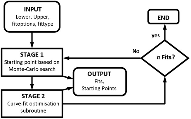
Computer algorithm for Blueprint XAS based on the methodology described herein (see text).
To allow for appropriate estimation of errors, the array of resulting fits, as well as the corresponding array of start points that lead to each fit, are saved to the output for further analysis. Included in this output is a set of goodness-of-fit parameters for each fit. The computed confidence intervals for every parameter in each fit are also included in the output. These confidence intervals, in principle, represent an estimation of the error associated with the computation of each fit. However, if a large number of fits is generated, the error associated with the fitting procedure is better represented by the standard deviation of the coefficients in the whole population of fits. (The error associated with each fit is systematically removed upon the creation of a large family of them.)
3. Descriptive example: the analysis of a linear pseudo data set
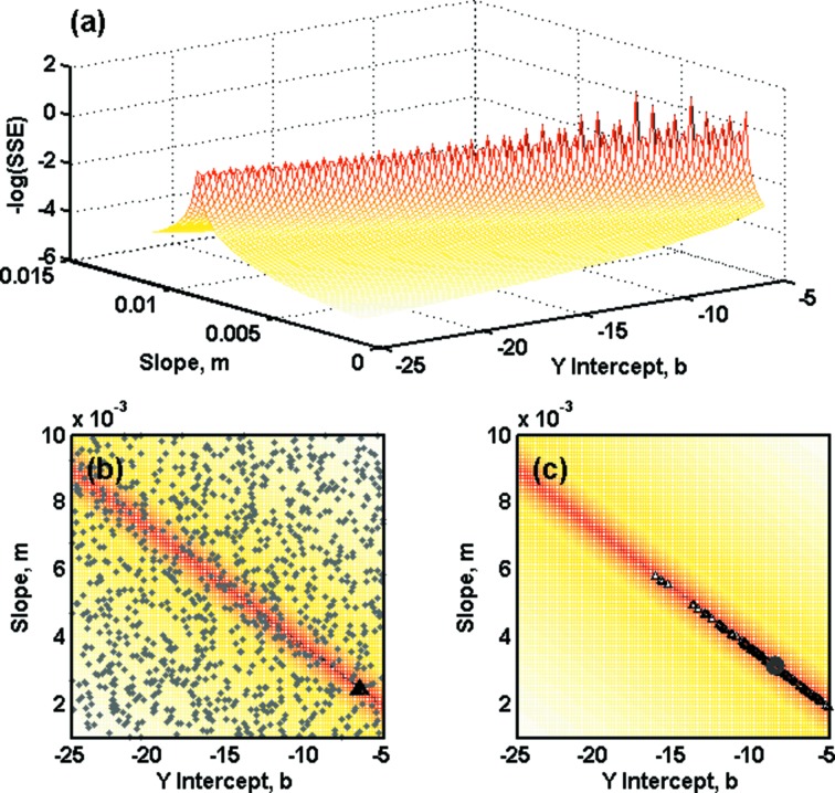
Fig. 2 ▶ illustrates the methodology with the use of a simple example. The example consists of the fitting of a pseudo data set using a linear evaluation function with parameters m (slope) and b (y intercept). The upper and lower bounds for m are set to 1 × 10⁻² and 1 × 10⁻³, respectively. The corresponding limits for b are set to −25 and −5. Since the example is simple enough, a surface can be created using a discrete but large number of combinations of m and b. The z-component of each point in the obtained mesh grid is defined as the corresponding −log(SSE) value and estimated upon the comparison of the evaluation function with the data using the values of m and b at each point of the grid. The solution to this particular problem sits on the maximum of the surface in Fig. 2(a) ▶. From this, it is also evident that there is a strong anti-correlation relationship between parameters m and b, as indicated by the belt of maxima sitting at high values of −log(SSE).
Figure 2.
Fitting of a straight line (with added random noise) using the methodology described in the text. (a) Solution via the evaluation of the fitting model using a discrete number of values of m and b. (b) Selection of the start point (black triangle) (out of a 1000 randomly generated points; grey dots) used in the computation of the first fit. (c) Selected start points used in the computation of 100 fits (grey triangles) and the final fit in all cases (black circle).
In a regular XAS evaluation function, the creation of an equivalent surface in order to find the solution (or solutions) is prohibitive, owing to the large number of fitting parameters. Figs. 2(b) and 2(c) ▶ illustrate the application of the methodology described above to the linear function of this example. The surface of Fig. 2(a) ▶ (seen from the top and projected into the xy plane) is embedded as a reference. A total of 100 fits are computed. The 1000 random combinations of values of m and b for one of the fits [grey dots in Fig. 2(b) ▶] clearly span the whole solution space. From these combinations, that with the lowest SSE [highest −log(SSE)] is selected as the starting point (represented by the black solid triangle) in the computation of that particular fit. In Fig. 2(c) ▶, the selected starting points for each of the computed fits are represented as hollow black triangles. The fact that practically all of these starting points lie on the anti-correlation belt region (with most of them near the solution) reflects the effectiveness of the Monte Carlo-based method, and confirms that the evaluation function is well behaved. Owing to the simplicity of this example, the solutions for the 100 fits are practically identical and are all represented by the dark grey solid circle in Fig. 2(c) ▶.
4. Analysis of experimental XAS data sets
The following examples show the applicability of the methodology described in the previous section, by using several real examples. Throughout these examples, the following issues are explored: (i) the number of fits required to ensure statistically meaningful solutions; (ii) the reproducibility and errors associated with the fitting procedure; (iii) the effects of concentration in solid samples and its implications; (iv) the possible propagation of errors upon background subtraction prior to the fitting procedure; and (v) the implementation of the methodology in multiple-edge XAS data.
The first four of these issues were investigated using the XAS data collected on several samples of tetragonal (NEt4)2CuCl4. The last issue was investigated using the Ru L-edge XAS spectrum of the chlorine-free compound 1 (Fig. 3 ▶), which has been used previously in our group as a reference for the development of the methodology used in the analysis of the Cl K- and Ru L 2,3-edges XAS data of ruthenium-based carbene catalysts (Delgado-Jaime et al., 2006 ▶).
Figure 3.
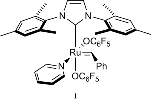
Structure of compound 1 (Conrad, Camm & Fogg, 2006 ▶; Conrad, Snelgrove et al., 2006 ▶).
4.1. Data collection and sample preparation
Tetragonal CuCl4 2− (i.e. with D 2d local symmetry) has become a commonly used compound to calibrate and extract covalency on chlorine-containing metal complexes. Copper chloride compounds have been subjected to several studies over the years (e.g. Glaser et al., 2000 ▶; Shadle et al., 1994 ▶) and therefore represents a good reference for the applicability of our methodology. We fitted and analyzed several data sets of solid (NEt4)2CuCl4 collected at different times over a five-year period. The first data set corresponds to two long-range scans, in the energy region from 2720 to 3150 eV, collected at beamline 6-2 of Stanford Synchrotron Radiation Lightsource (SSRL). The rest of the data, obtained from 14 different samples, correspond to shorter scans (two per sample) obtained more recently at beamline 4-3 of SSRL, in the energy range 2750–2900 eV. The data for compound 1 were also collected in the energy range from 2720 to 3150 eV at beamline 6-2. In all cases, fluorescence data were collected using a Lytle detector (filled with N2).
Samples were finely ground and diluted prior to data collection to reduce distortion effects. A common vehicle to dilute the solid samples to reduce self-absorption is boron nitride (BN), a highly dense material with little absorption in the relevant scanning region. In the case of (NEt4)2CuCl4, the sample used to collect the long-range scans was not diluted. However, the 14 samples used to collect the short-range scans were diluted using different approximate ratios BN:(NEt4)2CuCl4 (v:v), as indicated in Table 2. The sample used to scan the Ru L-edge XAS of compound 1 was finely ground but undiluted.
4.2. How many computed fits per job?
The possibility of having multiple good solutions to a particular fitting problem makes the generation of multiple independent fits a necessity. To investigate how many fits should be generally obtained when running a job in Blueprint XAS, the two long-range scans of (NEt4)2CuCl4 were averaged and the resulting data were fitted, using the evaluation function described in Fig. 1 of the supplementary information1. This evaluation function consisted of two pseudo-Voigt peaks to model the pre-edge and near-edge features, one cumulative pseudo-Voigt function to model the edge jump and a switch-like function to model the background. An internal normalization of the peaks was accomplished by defining the intensity of the pre-edge peak as a function of the edge jump intensity directly within the evaluation function (Delgado-Jaime et al., 2010 ▶).
A total of 10, 100, 1000 and 10000 fits were computed for the Cl K-edge XAS long-range data set on (NEt4)2CuCl4, in four separate jobs.
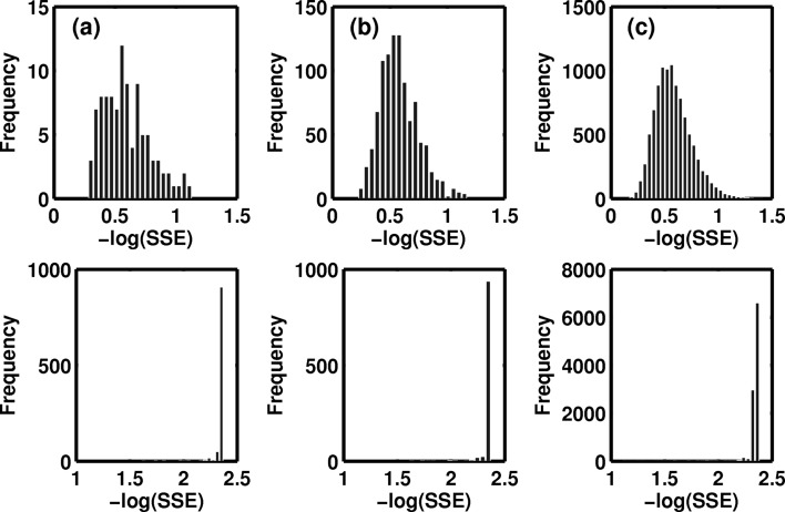
Table 1 ▶ lists the average and the standard deviation of relevant fitted parameters obtained from these fit jobs. Fig. 4 ▶ shows the distribution of the start points and the fits according to their −log(SSE) value for the last three fit jobs.
Table 1. Results for fit jobs involving (a) 10, (b) 100, (c) 1000 and (d) 10000 independent fits in the Cl K-edge XAS long-range data set of (NEt4)2CuCl4 .
| (a) 10 fits | (b) 100 fits | (c) 1000 fits | (d) 10000 fits | |||||
|---|---|---|---|---|---|---|---|---|
| Coefficient parameter† | Average | Std dev | Average | Std dev | Average | Std dev | Average | Std dev |
| Edge | ||||||||
| Intensity, I 1 | 0.246 | 0.001 | 0.245 | 0.001 | 0.245 | 0.001 | 0.245 | 0.001 |
| Energy position (eV), O 1 | 2824.90 | 0.74 | 2825.29 | 1.04 | 2825.24 | 1.00 | 2825.27 | 1.02 |
| Peak 1 | ||||||||
| Normalized intensity, I 2 | 0.577 | 0.004 | 0.578 | 0.008 | 0.579 | 0.008 | 0.579 | 0.009 |
| Energy position (eV), O 2 | 2820.16 | 0.01 | 2820.16 | 0.01 | 2820.16 | 0.01 | 2820.16 | 0.01 |
| Peak 2 | ||||||||
| Normalized intensity, I 3 | 2.57 | 0.83 | 3.02 | 1.16 | 2.96 | 1.12 | 2.99 | 1.14 |
| Energy position (eV), O 3 | 2826.40 | 0.13 | 2826.29 | 0.18 | 2826.30 | 0.18 | 2826.29 | 0.18 |
Parameter identifiers are as described in the corresponding evaluation function (Fig. S1).
Figure 4.
Distribution of start points (top) and fits (bottom) for fit jobs with (a) 100, (b) 1000 and (c) 10000 independent fits for the Cl K-edge XAS long-range data set of (NEt4)2CuCl4.
As is evident from Table 1 ▶, the average values for the parameters corresponding to more resolved features in the spectrum, such as the pre-edge intensity and the pre-edge energy position, are well defined when only ten fits are obtained. However, this sample size is not large enough to estimate errors in these parameters. The results in this table indicate that performing 100 fits gives rise to better defined average values in all the parameters as well as good estimates in their associated errors when compared with the more time- and resource-demanding jobs (c) and (d). Furthermore, Fig. 4 ▶ indicates that increasing the total number of fits improves the distribution profile of the start points when going from 100 to 10000 fits; yet it does little to change the statistical results in the actual fits. Therefore, the amount of time spent to compute 10000 fits in this case (8.5 days) is completely unnecessary. The results obtained from computing only 100 fits, which took only 2 h in this particular case, represent well the solution for this problem. We conclude from this that, in general, 100 fits should be sufficient in most relatively straightforward data sets to statistically explore the solution space of a fitting problem in XAS. However, we caution that more complex cases may require users to perform additional fits.
4.3. Reproducibility of fit jobs
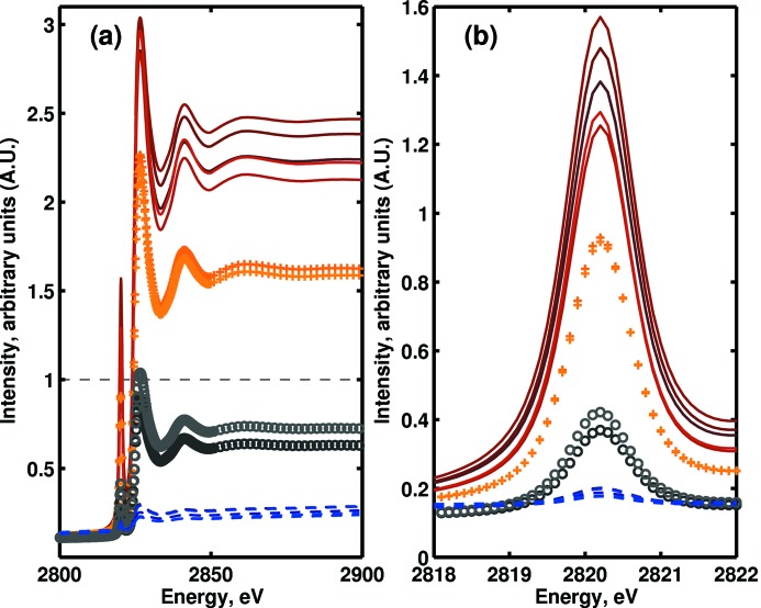
The two scans collected for each of the 14 (NEt4)2CuCl4 samples were averaged and the resulting data sets were calibrated by adjusting the maximum in the pre-edge peak to 2820.2 eV (Glaser et al., 2000 ▶; Shadle et al., 1994 ▶). The calibrated data sets are illustrated in Fig. 5 ▶. As indicated in Table 2 ▶, samples 1–5 were diluted with ∼50% of BN, samples 6–7 with ∼75% of BN, samples 8–9 with ∼90% and samples 10–14 with more than 90% of BN by volume. It is evident from this figure that the intensity of the spectral features correlates well with the concentration of chlorine in each sample.
Figure 5.
Calibrated data sets corresponding to the Cl K-edge XAS spectra for samples 1–14 of (NEt4)2CuCl4 in (a) the entire scanned region and (b) the pre-edge region. Data sets corresponding to samples with 50% of BN are displayed as solid lines in different shades of red (darker to lighter on going from 1 to 5 in Table 2 ▶); data sets corresponding to samples with 75% of BN are displayed in different shades of orange plus signs (darker to lighter on going from 6–7 in Table 2 ▶); data sets corresponding to samples with 90% of BN are displayed as hollow circles in different shades of grey (darker to lighter on going from 8–9 in Table 2 ▶); and data sets corresponding to samples with more than 90% of BN are displayed as dashed lines in different shades of blue (darker to lighter on going from 10–14 in Table 2 ▶).
Table 2. Results for pre-edge parameters from the fitting of Cl K-edge XAS data sets 114 of (NEt4)2CuCl4 .
| Normalized intensity | Energy position (eV) | Width (HWHM) (eV) | Shape (% Gaussian) | ||||
|---|---|---|---|---|---|---|---|
| Lower | Upper | Lower | Upper | Lower | Upper | Lower | Upper |
| 0.2 | 1.5 | 2820 | 2821 | 0.1 | 4 | 0 | 100 |
| Sample | Normalized intensity | Energy position (eV) | Width (HWHM) (eV) | Shape (% Gaussian) | |||||
|---|---|---|---|---|---|---|---|---|---|
| # | % BN | Average | Std dev | Average | Std dev | Average | Std dev | Average | Std dev |
| 1 | 50 | 0.846 | 0.007 | 2820.20 | 0.01 | 0.508 | 0.006 | 18.8 | 0.9 |
| 2 | 50 | 0.846 | 0.010 | 2820.20 | 0.01 | 0.512 | 0.006 | 19.2 | 1.7 |
| 3 | 50 | 0.918 | 0.018 | 2820.20 | 0.01 | 0.535 | 0.004 | 20.0 | 0.4 |
| 4 | 50 | 0.768 | 0.004 | 2820.20 | 0.01 | 0.497 | 0.001 | 22.9 | 0.3 |
| 5 | 50 | 0.762 | 0.007 | 2820.19 | 0.01 | 0.499 | 0.006 | 23.5 | 1.2 |
| 6 | 75 | 0.701 | 0.009 | 2820.20 | 0.01 | 0.499 | 0.001 | 27.1 | 0.1 |
| 7 | 75 | 0.715 | 0.045 | 2820.21 | 0.01 | 0.496 | 0.003 | 26.3 | 7.9 |
| 8 | 90 | 0.614 | 0.069 | 2820.20 | 0.01 | 0.485 | 0.017 | 32.2 | 11.7 |
| 9 | 90 | 0.630 | 0.058 | 2820.19 | 0.01 | 0.487 | 0.013 | 30.0 | 8.6 |
| 10 | >90 | 0.650 | 0.067 | 2820.21 | 0.07 | 0.512 | 0.224 | 30.9 | 12.1 |
| 11 | >90 | 0.596 | 0.074 | 2820.21 | 0.08 | 0.506 | 0.122 | 34.9 | 12.3 |
| 12 | >90 | 0.569 | 0.060 | 2820.22 | 0.11 | 0.557 | 0.495 | 46.7 | 13.0 |
| 13 | >90 | 0.702 | 0.030 | 2820.22 | 0.03 | 0.497 | 0.014 | 27.6 | 7.9 |
| 14 | >90 | 0.565 | 0.067 | 2820.22 | 0.08 | 0.525 | 0.222 | 47.9 | 14.4 |
The evaluation function used to fit these data sets was the same in all cases, but different to the one used to fit the long-range data set discussed in the previous section. The simplified model used in this case excludes the data around the tip of the second peak (2825–2828.5 eV; Fig. S3 of supplementary information) and removes the corresponding peak function from the evaluation function, f (Fig. S2 of supplementary information). Under these circumstances the results from the corresponding fit jobs are inadequate for estimating the edge position, as the removal of the second peak from the model has the effect of moving the edge to lower energies. Furthermore, the edge intensity is inherently more inaccurate for these data sets, given the fact that the data scans do not go beyond 2900 eV, which otherwise would allow a better definition of the overall structure of the edge jump. In other words, the results for the edge jump parameters, although consistent among all data sets, are unimportant and not the main focus in this section. Instead, the obtained results were used exclusively to compare the normalized intensity of the pre-edge feature between the different data sets.
For each data set, a fit job consisting of 100 fits was computed, using the same lower and upper bounds in all cases. The numerical results for the parameters of the pre-edge feature are listed in Table 2 ▶.
To check for reproducibility, four additional fit jobs (with 100 fits each) were obtained for samples 1 and 3 and the results for the parameters on the pre-edge feature are reported in Table S4 (of the supplementary information). The behaviour of the variability of these results among the different fit jobs is illustrated in Fig. S5 (of the supplementary information) indicating that the methodology described here is robust and reproducible.
4.4. Concentration effects
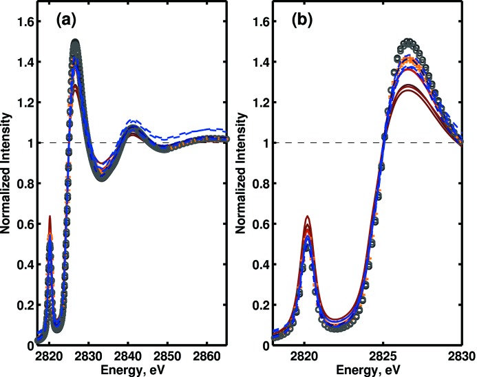
To graphically compare the results obtained from the 14 data sets on (NEt4)2CuCl4, the background subtraction and normalization of each data set is accomplished within Blueprint XAS by using the post-fitting toolbox (Delgado-Jaime et al., 2010 ▶). From Fig. 6 ▶, it is evident that by diluting the sample with BN the intensity of the pre-edge peak decreases while the near-edge peak feature increases.
Figure 6.
Background subtraction and normalization of data sets 1–14 in (a) the entire scanned region and (b) the pre-edge region. Colour and line style coding are as indicated in Fig. 5 ▶.
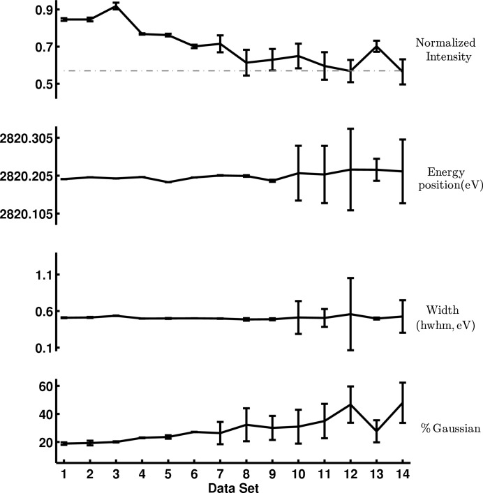
The numerical results directly obtained for the pre-edge normalized intensity indicate the same trend (Table 2 ▶). Along the series of data sets 1–14, a clear decrease in the normalized intensity of the pre-edge is observed (Fig. 7 ▶). Additionally, the width seems to remain constant with a small tendency to decrease, whereas the shape of the peak becomes slightly more Gaussian.
Figure 7.
Variation of pre-edge parameters according to the fit results on the Cl K-edge XAS data sets 1–14 of (NEt4)2CuCl4.
Interestingly, as the concentration of BN becomes higher, the uncertainty in the four coefficients increases. Specifically, in the most dilute samples (from 8 to 14), the uncertainty on the peak position is significantly increased. This is due to the fact that as the samples becomes more diluted the influence of the background becomes more important, as suggested also by Fig. S6 (of the supplementary information), particularly in the case of the most dilute samples 10–14, for which the pre-edge region of the background increases its steepness significantly. These results imply that background subtraction and normalization procedures prior to fitting, especially for spectra of dilute samples, may introduce important errors in the fit parameters.
The observed differences in the normalized intensity of the pre-edge through the series are attributed to self-absorption effects. In relatively concentrated samples, the edge jump is so intense that it becomes saturated in relation to the less-intense pre-edge feature. As observed, this effect becomes less important once the sample becomes significantly diluted. This has been discussed in detail previously for the case of S K-edge XAS of S8 (George et al., 2008 ▶). Samples with an inherently high concentration of the absorbing element [100% of sulfur in S8; and ∼30% of Cl in (NEt4)2CuCl4 by mass] are prone to important distortion effects when the data sets come from solid samples that are concentrated and whose particle size is relatively large. For the case of (NEt4)2CuCl4, the somewhat asymptotic behaviour of the plot for the normalized intensity at high proportions of BN (>90%) in Fig. 7 ▶ indicates that self-absorption effects are attenuated at this level of dilution.
Previous studies on the Cl K-edge XAS spectrum of tetragonal CuCl4 2− have provided an estimate on the covalency of Cu—Cl (Shadle et al., 1994 ▶; Glaser et al., 2000 ▶). In these studies, no sample dilution was performed, although a somewhat equivalent procedure was carried out to minimize possible self-absorption and anisotropic effects. This procedure was based on the analysis of the raw data obtained from several samples that were spread out over Mylar tape with increasingly thinner sample thickness. Furthermore, their fitting analysis was based on a few manually performed independent fits using traditional background subtraction and normalization procedures. An intensity of 0.57 was found for the pre-edge feature (dash-dotted grey line in Fig. 7 ▶), which generally agrees with our data from diluted samples within error. However, we note that the inherent uncertainty in the fitting procedure leads to a relatively large, and heretofore unaccounted for, error in the reference value. The importance of this factor requires further investigation.
5. Multi-edge fitting
The fitting of the Ru L 2,3 XAS data for compound 1 is used (i) to demonstrate the applicability and robustness of the switch-like background model (see Appendix A ) and (ii) to show the application of the methodology when fitting multiple-edge spectra with several shared parameters.
In recent years, the exploration of L-edge XAS in second-row transition metal complexes has grown significantly (e.g. Boysen & Szilagyi, 2008 ▶; Harris et al., 2009 ▶). While having a complicated background in these cases is generally perceived as a challenge, the double-edge spectrum under almost jj-coupling conditions can also be beneficial in the fitting of this and other similar data.
A previous study using a different function to model the background, and a traditional approach to analyse the data set of compound 1 (Delgado-Jaime et al., 2006 ▶), suggested that the branching ratio between the L 3 and L 2 edges differs markedly from the statistical 2:1 ratio.
As a starting procedure, Fig. 8 ▶ illustrates a rough graphical manipulation of the Ru L 2,3 XAS data of compound 1 used in these studies. The proportion between the two edge jumps and between the total intensity of the pre-edge and near edge features in the two edges obeys a branching ratio of ∼1.7. This is not exclusive of compound 1, but rather a more general observation for other second-row transition-metal complexes (Hu et al., 2000 ▶).
Figure 8.
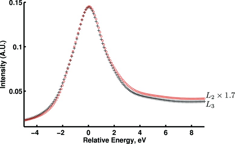
Rough graphical manipulation of the raw Ru L 2,3 XAS spectra for compound 1. The energy scale is relative to the maximum of the pre-edge feature in L 3 (black plus signs centred at ∼2842 eV) and to the maximum of the pre-edge feature in L 2 (red hollow circles centred at ∼2842 + 128.7 eV). The intensity of the L 2 edge is rescaled using a factor of 1.7.
The formulation of an evaluation function for the fitting of this and similar data becomes simpler when considering these observations. A unique parameter (B 1, Fig. 9 ▶) that relates the intensity of the two edge jump functions as well as the intensity of the two clusters of peaks in the two edges can be used. It is therefore extremely useful for the evaluation function to make use of global and shared parameters, which is straightforward in our implementation.
Figure 9.
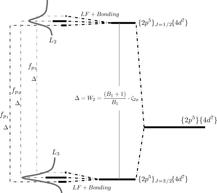
Energy correlation between the position of the edges and the peak features in L 2,3-edges XAS under almost jj-coupling conditions, for which the dominant interaction is the 2p spin–orbit coupling. The remaining interactions can be considered as perturbations of the same magnitude for each edge.
Based on these considerations, a relatively simple evaluation function (see Fig. S7 in the supplementary information for details) is constructed. In this case the sharing of parameters within the evaluation function imposes significant a priori constraints that simplify the overall fitting procedure even more than would generally be anticipated from simply decreasing the total number of parameters in the non-linear least-squares fitting procedure. To further simplify the evaluation function, the shape and width of the duplicate functions of the L 2 edge were set to be identical to those in the L 3 edge. This last simplification may not always be suitable in the fitting of such spectra, although it seems to be a generally reasonable starting point when first developing the fit model.
The evaluation function can also be further simplified by noting that the energy separation between the inflection points of the two edges should, in principle, be the same as the separation of equivalent peak features between the two edges, as shown in Fig. 9 ▶. In general, this is a very likely simplification of the problem under near jj-coupling conditions in which the atomic, the ligand field and the bonding interactions that occur in one edge, or the other, are of the same magnitude provided the interaction of the 2p core hole with the 4d shell is negligible. As suggested by Fig. 8 ▶, this should be the case for compound 1.
The final evaluation function used for the fitting of the Ru L 2,3-edges XAS spectrum of compound 1 thus resulted in a model with a total of 18 parameters (see Fig. S8 in the supplementary information). Equivalent features in each of the edges were linked using a global energy splitting (Δ = W 2 in Fig. 9 ▶). Using this evaluation function, three fit jobs (to check for reproducibility) with 100 fits each were computed. The results for relevant parameters are listed in Table 3 ▶.
Table 3. Relevant parameters in the fitting of the Ru L 2,3-edges XAS spectrum of compound 1 .
| Limits | Fit job #1 | Fit job #2 | Fit job #3 | |||||
|---|---|---|---|---|---|---|---|---|
| Coefficient parameter† | Lower | Upper | Average | Std dev | Average | Std dev | Average | Std dev |
| Branching ratio, B 1 | 1.3 | 2.5 | 1.73 | 0.01 | 1.73 | 0.02 | 1.73 | 0.05 |
| W 2 | 128 | 130 | 128.7 | 0.1 | 128.7 | 0.1 | 128.7 | 0.1 |
| L 3-edge | ||||||||
| Inflection point, O 1 | 2837 | 2843 | 2841.7 | 0.8 | 2841.7 | 0.6 | 2841.7 | 0.7 |
| Shape, G 1 | 0 | 100 | 33.0 | 20.4 | 34.7 | 21.0 | 30.8 | 17.4 |
| Width, W 1 | 0.1 | 3 | 1.79 | 0.61 | 1.70 | 0.73 | 1.78 | 0.67 |
| Peaks | ||||||||
| Shape, G 2 | 0 | 100 | 18.4 | 8.8 | 19.4 | 7.5 | 18.1 | 5.8 |
| Width, W 3 | 0.05 | 3 | 1.28 | 0.10 | 1.30 | 0.12 | 1.28 | 0.10 |
| f p1 | ||||||||
| Relative position, O 6 ‡ | 2.5 | 0.5 | 1.3 | 0.4 | 1.3 | 0.5 | 1.3 | 0.4 |
| Relative intensity, B 2 § | 0 | 1 | 0.236 | 0.206 | 0.209 | 0.169 | 0.224 | 0.166 |
| f p2 | ||||||||
| Position, O 4 | 2841 | 2843 | 2842.0 | 0.1 | 2842.0 | 0.1 | 2842.0 | 0.1 |
| Normalized intensity, I 2 | 2 | 20 | 12.7 | 1.9 | 13.2 | 1.7 | 13.1 | 1.6 |
| f p3 | ||||||||
| Relative position, O 7 ‡ | 0.5 | 3 | 1.6 | 0.5 | 1.6 | 0.5 | 1.6 | 0.4 |
| Relative intensity, B 3 ‡ | 0 | 1 | 0.185 | 0.196 | 0.165 | 0.171 | 0.151 | 0.132 |
Parameter identifiers are as described in the corresponding evaluation function (Fig. S8 of supplementary information).
Energy position relative to energy position of f p2(O 4).
Intensity relative and defined as a of of the normalized intensity of f p2 (I 2).
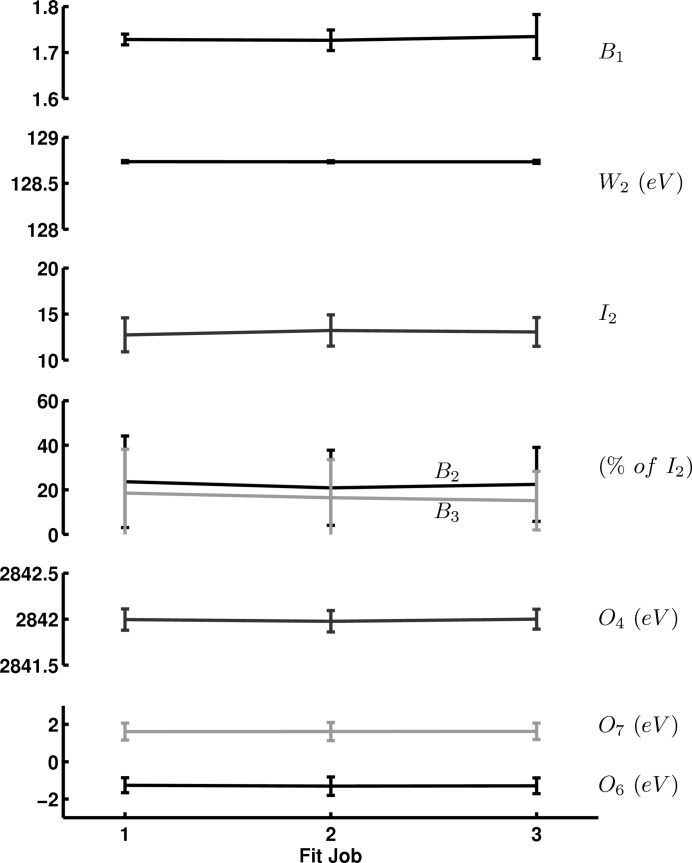
The variability of W 2 is minimal and practically the same as in ruthenium metal (∼129 eV) (Williams, 2001 ▶). This implies that possible interactions of the valence shell with the 2p core hole in the ruthenium metal, or in other words that of the spin–orbit coupling of the 2p shell of ruthenium (II) in compound 1, is essentially the same as for ruthenium metal. Conversely, a large variability is observed for the parameters of the three peak functions in the fits of the three jobs, particularly the intensity, as evidenced by the results in Table 3 ▶ and Fig. 10 ▶. In situations like this, in which a pre-edge or near-edge feature is not well resolved, the data set is not good enough to yield a simple solution based on a unique or even a few independent fits.
Figure 10.
Variability of relevant parameters in the fitting of Ru L 2,3-edges XAS data of compound 1, among the three fit jobs performed using the evaluation function of Fig. S7.
In a previous manuscript, we reported, based on a broad set of fits performed manually using a traditional fitting methodology, the branching ratio between the intensities of the two edges as Ru L 3/L 2 = 1.74 (Delgado-Jaime et al., 2006 ▶). Herein, the value for this parameter, which was also used to correlate the intensities of equivalent peak features in the two edges, is in close agreement with B 1 = 1.73 ± 0.05.
The same methodology discussed in this section can be easily employed to explore more complicated cases, allowing for a robust and methodical approach to identify whether meaningful chemical information may be effectively extracted from a specific data set. For example, we point to the overlap between Ru L 2,3-edges and Cl K-edges as a cause of concern for the investigation of ruthenium-based olefin metathesis catalysts (Delgado-Jaime et al., 2006 ▶; Getty et al., 2007 ▶) as well as in ruthenium-containing anti-cancer targets (Harris et al., 2009 ▶; Sriskandakumar et al., 2009 ▶). Furthermore, this model can be also used to check for possible distortions in the data, in the sense that if the evaluation function does not seem to fit a particular set properly it might very well be due to the presence of important distortions in one or more features, or else due to the presence of impurities.
6. Conclusions
A new methodology for the fitting of XAS data has been introduced and tested using several examples. The methodology differs from existing approaches in that it allows for simultaneous fitting of the background and spectroscopic features. To minimize parameters, we also propose a new edge-coupled background function that minimizes the number of fit parameters. Lastly, a Monte Carlo subroutine allows the XAS user to generate any number of independent fits with the introduction of minimal user bias. This methodology is used to explore a number of examples specifically addressing (i) the need to explore a broad solution space when evaluating a fit model (evaluation function); (ii) the potential effect of sequential background subtraction, normalization and peak fitting on the estimation of normalized intensities; (iii) the nature of the uncertainty in XAS near-edge data analysis; (iv) the exploration of possible distortions effects; and (v) the exploration of the reproducibility of fit jobs and robustness of the evaluation function. Our results suggest that fitting (rather than subtracting in a preliminary step) the background is necessary to avoid biased solutions and propagation of errors in the analysis of near-edge XAS data. Furthermore, in many cases, the information contained in XAS data may not be as easily deconvoluted as our own bias may suggest. In such cases, large uncertainties should be anticipated and can be addressed more explicitly. In our newly developed approach, uncertainties in the fitting of a data set are immediately apparent and provide the user with detailed information regarding the limitations of the fitting procedure.
Supplementary Material
Supporting information file. DOI: 10.1107/S090904950904655X/ot5602sup1.pdf
Acknowledgments
This research is funded by NSERC (the Natural Science and Engineering Research Council of Canada); infrastructure support provided by UBC. Special thanks from one of the authors (MUDJ) whose graduate fellowship is supported by funds from CONACYT (Consejo Nacional de Ciencia y Tecnología, México). Data analysis was performed on infrastructure funded by CFI and BCKDF through the Centre for Higher Order Structure Elucidation (CHORSE). Portions of this research were carried out at SSRL, a national user facility operated by Stanford University on behalf of the US DOE-BES. The SSRL Structural Molecular Biology Program is supported by DOE, Office of Biological and Environmental Research, and by the NIH, National Center for Research Resources, Biomedical Technology Program.
Appendix A. The switch-like background model
Previously, we reported a methodology to fit and/or subtract the background from multiple-edged XAS spectra (Delgado-Jaime et al., 2006 ▶). This method was based on an energy-weighting sum of parent functions, each fitting certain regions of the background model. Herein, we introduce an alternative model that uses fewer parameters and links some of these parameters to those of an edge.
The functional form of this new model (referred to here as the switch-like background model) is given by
Like in the case of the previously developed model, each term in this summation is constituted by the parent function (f i) corresponding to a particular quasi-linear region (with adjusted Y intercept) and by a factor, which in this case is a set of two unit step functions that act as switches. The first unit step function switches ‘on’ the parent function at a given value of energy b 1,i, whereas the second one switches ‘off’ the function above a second higher value of energy, b 2,i. Each of these switches uses an approximation to the Heaviside’s unit step function.
The Heaviside’s unit step function is defined by
 |
To provide a smoother change between background functions, the formal definition of the unit step function is not used in our model. Instead the Fermi–Dirac–Boltzmann cumulative distribution function is employed as a close approximation. The smoothness of the switch is provided by an additional width parameter (w). The functional form of this approximation to the unit step function is thus written as
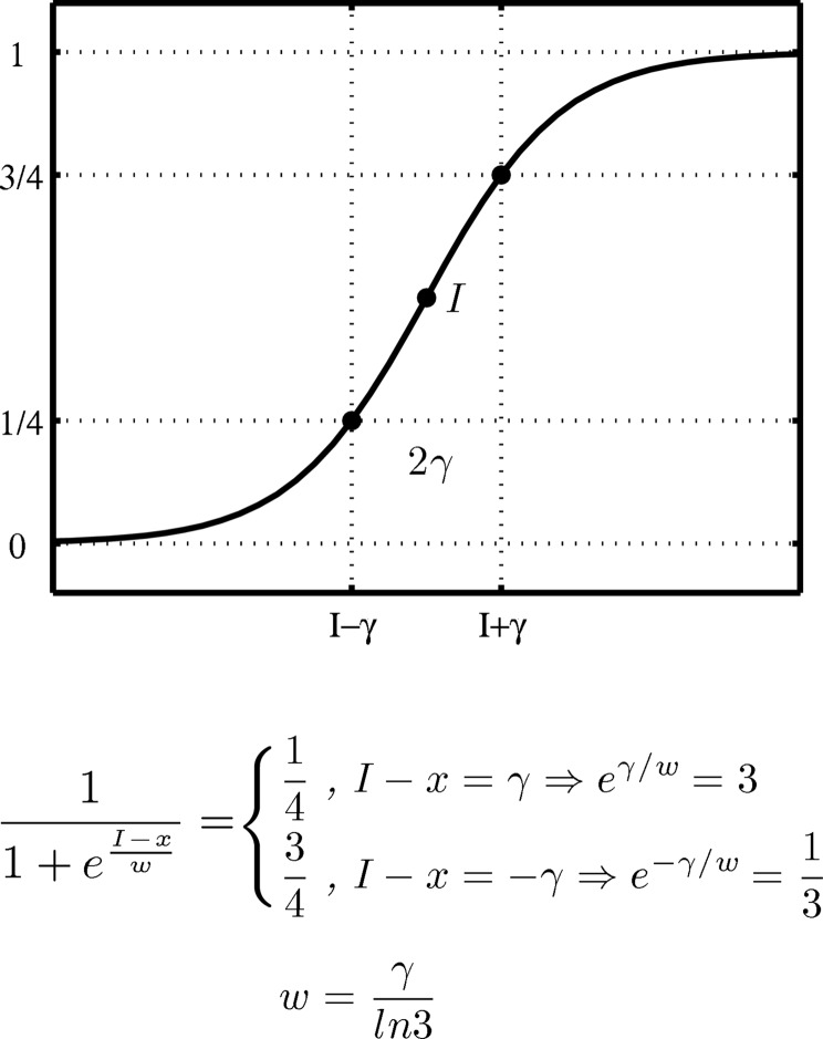
According to the demonstration given in Fig. 11 ▶, this approximation can be expressed in terms of the half width (γ) at half-maximum (HWHM), as follows,
Given that the functional form of the edge jump can also be modelled with a parameter related to the HWHM, using a single parameter to describe the smoothness of the transition between parent functions in the background and the width of an edge jump is extremely appealing. Moreover, and assuming that the change in the background in XAS is effected by an edge jump, the inflection point of an edge jump can be further linked to the transition energies between parent functions in the background, as shown in Fig. 12 ▶.
Figure 11.
Relationship between the generic width parameter (w) and γ (HWHM) in the approximation to the unit step function based on the Fermi–Dirac–Boltzmann profile.
Figure 12.
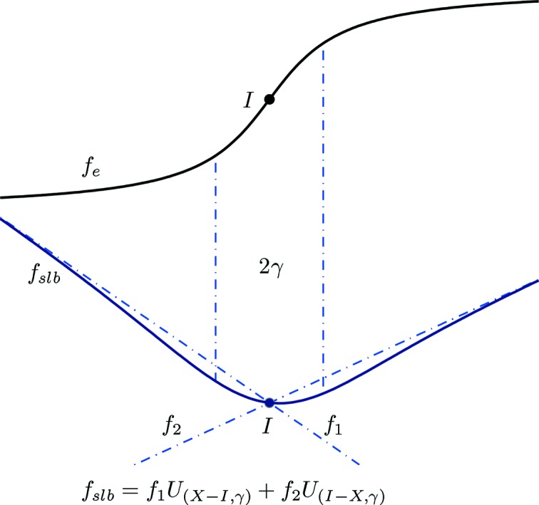
Half width at half-maximum (γ) and inflection point (I) of the edge function (f e, black solid line) and related properties in the associated background function (f b, grey solid line). The relative change in steepness of the features are accentuated for clarity.
Footnotes
Supplementary data for this paper are available from the IUCr electronic archives (Reference: OT5602). Services for accessing these data are described at the back of the journal.
References
- Boysen, R. B. & Szilagyi, R. K. (2008). Inorg. Chim. Acta, 361, 1047–1058.
- Conrad, J. C., Camm, K. D. & Fogg, D. E. (2006). Inorg. Chim. Acta, 359, 1967–1973.
- Conrad, J. C., Snelgrove, J. L., Eeelman, M. D., Hall, S. & Fogg, D. E. (2006). J. Mol. Catal. A, 254, 105–110.
- Curis, E. & Bénazeth, S. (2000). J. Synchrotron Rad. 7, 262–266. [DOI] [PubMed]
- Curis, E. & Bénazeth, S. (2005). J. Synchrotron Rad. 12, 361–373. [DOI] [PubMed]
- Curis, E., Osán, J., Falkenberg, G., Bénazeth, S. & Török, S. (2005). Spectrochim. Acta B, 60, 841–849.
- Delgado-Jaime, M. U., Conrad, J. C., Fogg, D. E. & Kennepohl, P. (2006). Inorg. Chim. Acta, 359, 3042–3047.
- Delgado-Jaime, M. U., Mewis, C. & Kennepohl, P. (2010). J. Synchrotron Rad. 17, 132–137. [DOI] [PubMed]
- George, G. N., Gnida, M., Bazylinski, D. A., Prince, R. C. & Pickering, I. J. (2008). J. Bacteriol. 190, 6376–6383. [DOI] [PMC free article] [PubMed]
- Getty, K., Delgado-Jaime, M. U. & Kennepohl, P. (2007). J. Am. Chem. Soc. 129, 15774–15776. [DOI] [PubMed]
- Glaser, T., Hedman, B., Hodgson, K. O. & Solomon, E. I. (2000). Acc. Chem. Res. 33, 859–868. [DOI] [PubMed]
- Harris, T. V., Szilagyi, R. K. & McFarlane-Holman, K. L. (2009). J. Biol. Inorg. Chem. 14, 891–898. [DOI] [PubMed]
- Hu, H., von Lips, H., Golden, M. S., Fink, J., Kaindl, G., de Groot, F. M. F., Ebbinghaus, S. & Reller, A. (2000). Phys. Rev. B, 61, 5262–5266.
- Shadle, S. E., Hedman, B., Hodgson, K. O. & Solomon, E. I. (1994). Inorg. Chem. 33, 4235–4244.
- Sriskandakumar, T., Petzold, H., Bruijnincx, P., Habtemariam, A., Sadler, P. J. & Kennepohl, P. (2009). J. Am. Chem. Soc. 131, 13355–13361. [DOI] [PubMed]
- Weng, T.-C., Waldo, G. S. & Penner-Hahn, J. E. (2005). J. Synchrotron Rad. 12, 506–510. [DOI] [PubMed]
- Williams, G. P. (2001). X-ray Properties of the Elements, X-ray Data Booklet, edited by A. C. Thompson and D. Vaughan, pp. 1.1–1.8. Berkeley: Lawrence Berkeley National Laboratory.
Associated Data
This section collects any data citations, data availability statements, or supplementary materials included in this article.
Supplementary Materials
Supporting information file. DOI: 10.1107/S090904950904655X/ot5602sup1.pdf


