Reproduction is adapted to survival characteristics across geographically isolated medfly populations

Abstract

We propose the hypothesis that individual longitudinal trajectories of fertility are closely coupled to varying survival schedules across geographically isolated populations of the same species, in such a way that peak reproduction takes place before substantial increases in mortality are observed. This reproductive adaptation hypothesis is investigated for medflies through a statistical analysis of biodemographic data that were obtained for female medflies from six geographically far apart regions. The following results support the hypothesis: (i) both survival and reproductive schedules differ substantially between these populations, where early peaks and subsequently fast declining reproduction are observed for short-lived and protracted reproductive schedules for long-lived flies; (ii) when statistically adjusting reproduction for the observed differences in survival, the differences in reproductive schedules largely vanish, and thus the observed differences in fertility across the populations can be explained by differences in population-specific longevity; and (iii) specific survival patterns of the medflies belonging to a specific population predict the individual reproductive schedule for the flies in this population. The analysis is based on innovative statistical tools from functional data analysis. Our findings are consistent with an adaptive mechanism whereby trajectories of fertility evolve in response to specific constraints inherent in the population survival schedules.

1. Introduction

Relating the biodemographic characteristics of survival and fertility for isolated populations of the same species that are found at various geographical locales allows the study of the forces that shape fertility. We study these relationships for Mediterranean fruitflies (Ceratitis capitata). Populations from geographically distant locales (referred to as biotypes) reflect local adaptations and genetic differences that are consequences of local characteristic features and of geographical separation. Patterns and changes in fertility may cause growth or decline of populations. Complex interactions have been found to exist between individual fertility and individual survival, and much research has been devoted to elucidate a ‘cost of reproduction’ in which intensive reproduction leads to reduced remaining lifespan, jeopardizing the longevity of highly fertile individuals (Partridge & Harvey 1985). A close association between the dynamics of decreases in egg-laying for individual medflies and their impending death was found in Müller et al. (2001), suggesting that individual egg supplies are typically depleted at the time of death.

Recent findings that optimal diet levels and compositions differ between optimizing survival and optimizing fertility (Carey et al. 2008) also point to complex interactions at the individual level. We study the question whether patterns of population survival influence fertility. Specifically, we investigate in which way individual reproductive trajectories are shaped by survival schedules that vary across populations. Such variations may reflect genetic drift or population-specific external influences or a combination of both. The reproductive adaptation hypothesis is a consequence of the premise that optimization of reproductive success necessitates that individual reproductive schedules are influenced by the population survival schedule. For example, repositioning periods of intensive reproductive activity and associated reproductive peaks earlier in life for flies in populations with frequent occurrence of early death is an adaptive strategy that will result in maximizing overall egg output. The alternative (formally corresponding to the statistical null hypothesis) is that individual reproductive schedules are not adapted to population survival schedules.

Six isolated populations (biotypes) of medflies were studied by assessing both survival at the population level and temporal fertility trajectories at the individual level, measured in terms of daily egg-laying, representing the following regions: Africa (Kenya), Pacific (Hawaii), Central America (Guatemala), South America (Brazil), Western Mediterranean (Portugal) and Eastern Mediterranean (Greece). These data have been analysed by traditional demographic methods in Diamantidis et al. (2009). For each biotype, 50 female medflies were randomly selected and raised in the laboratory under defined conditions (for details, see Diamantidis et al. 2009). Daily egg counts for each individual fly until death and its age-at-death were recorded. One fly was deleted from the sample as its egg-laying pattern was clearly outlying. Two groupings emerged, biotypes with short-lived females (Kenya, Hawaii and Guatemala; life expectancy at eclosion 48–58 days) and those with long-lived females (Greece, Portugal and Brazil; life expectancy 72–76 days). Inasmuch as the Brazilian biotypes were collected in the interior of the state of Bahia, which experiences nearly six months of extremely low rainfall, much like the climates in which Portuguese and Greek biotypes were collected, the short- and long-lived groups can also be cross-classified as belonging to tropical and Mediterranean-like climates, respectively.

Since individual medfly fertility is constrained by an individual's survival, and as population growth depends on population fertility, we postulate the reproductive adaptation hypothesis that the temporal patterns of individual fertility schedules are influenced by the population survival schedule. That is, at the individual level, reproduction (egg-laying) must take place before the individual's death, where the latter is governed by the population survival schedule, to ensure successful reproduction of the individual. It is therefore probable that at the population level, the ensemble of individual trajectories of fertility is affected by the survival schedule of the population. Adjusting reproductive trajectories in response to evolving survival schedules is expected to be especially relevant for invading species which evolve life-history traits regularly in adaptation to new environments or as a consequence of genetic drift (Lee 2002; Duyck et al. 2007).

We study these issues using data collected as described in Diamantidis et al. (2009) and demonstrate the usefulness of functional data analysis methods for quantitative studies of biological trajectories, expanding on the approaches of Kirkpatrick & Heckman (1989) and Gomulkiewicz & Kingsolver (2007). In particular, we will demonstrate the functional regression technique (Ramsay & Dalzell 1991; Ramsay & Silverman 2005; Yao et al. 2005) to investigate the reproductive adaptation hypothesis.

2. Reproductive trajectories for medfly populations, adjusted and unadjusted for survival

It proves useful to quantify the survival schedules through population hazard rates (force of mortality). To investigate whether survival shapes reproduction, two subsamples were created from the original cohorts: a survival-adjusted and an unadjusted sample. The survival-adjusted sample was obtained by constrained randomization such that all cohorts have the same number of deaths in every 5 day interval. This type of adjustment is inspired by weighted bootstrap alignment through distribution tilting (Hall et al. 2008). We obtained a survival-adjusted sample of size 54 (nine flies from each population). An unadjusted sample, including another 54 flies with nine flies from each population, was assembled by unconstrained randomization from the remaining flies that had not been selected for the survival-adjusted samples.

Large differences in reproductive schedules between the short-lived and the long-lived cohorts are evident when one compares the estimated mean functions of the unadjusted samples (figure 1a). These differences are substantially reduced in the survival-adjusted samples (figure 1b). To confirm these empirical observations, functional data analysis methodology was applied to the combined survival-adjusted and unadjusted samples. This analysis was based on the first two functional principal components, which were calculated for all individual reproductive trajectories in the combined sample and serve as summaries of their shapes, without requiring any model shape assumptions (see the electronic supplementary material for details).

Figure 1.

Estimated mean reproductive functions for (a) the selected survival-unadjusted and (b) survival-adjusted samples. In both (a,b), the thinner black lines represent the short-lived cohorts (solid line, Guatemala; dashed line, Kenya; dash-dot line, Hawaii) and the thicker grey lines represent the longer lived cohorts (solid line, Greece; dashed line, Portugal; dash-dot line, Brazil).

Effects of adjustment (comparing survival-adjusted and unadjusted groups) and additional effects of survival characteristics that are independent of the adjustment (comparing short-lived and long-lived groups) on the shape of reproductive trajectories were assessed by fitting a multivariate multiple linear regression model,

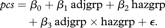2.1

The response pcs is the vector consisting of the first two functional principal components of the fertility trajectories, considered on a domain from 0 to 62 days. This domain was chosen for fertility trajectories throughout to avoid tail problems caused by differences in survival.

The functional principal components vary across individual flies and reflect the shape of individual egg-laying trajectories. They can be interpreted in conjunction with the shapes of the mean function and the first two eigenfunctions (for details, see the electronic supplementary material, equations (3) and (5), where K = 2 components are included). The eigenfunctions characterize the entire population and are visualized in figure 2b, while the overall mean function across all samples is in figure 2a. The predictor variables are indicators, where adjgrp is the indicator for survival adjustment and hazgrp is the indicator for the population characteristic of long or short lived. Here, adjgrp = 1 when the fly is in the unadjusted cohort (otherwise = 0) and hazgrp = 1 if the fly is from Greece, Portugal and Brazil (long-lived group), so that the survival-adjusted cohorts from Guatemala, Kenya and Hawaii (short-lived group) serve as baseline (adjgrp = 0, hazgrp = 0). The term at β₃ is an interaction term between adjgrp and hazgrp and only has an effect when both indicators are at level 1, i.e. for the unadjusted long-lived group.

Figure 2.

(a) Estimated mean function and (b) the first three eigenfunctions for the combined survival-adjusted and unadjusted samples of fertility trajectories. First (solid line), second (dashed line) and third (dash-dot line) eigenfunctions explain 44.87, 35.52 and 9.22% of the total variation, respectively.

The overall MANOVA for the regression has a p-value of p < 0.001, indicating significant predictor effects. Specifically, predictors adjgrp and hazgrp have a significant impact on the first functional principal component ζ₁ through the interaction term, but not on the second component ζ₂, as shown in table 1. For the second component, the effect of hazgrp comes close to significance, so that it is possible that there are residual differences in fertility that are not entirely accounted for by the adjustment for survival. These residual differences would manifest themselves in the negative direction (because the coefficient in the regression model is negative) of the second eigenfunction (see figure 2b). This eigenfunction reflects variation in the trajectories that is characterized by a broad peak in fertility around day 15, crossing the zero line and broadly negative effects on fertility thereafter. A negative version of this eigenfunction shape is more prominently represented in the fertility trajectories of the long-lived group, corresponding to less early reproduction and enhanced later reproduction in the manner of the inverse shape of the second eigenfunction in figure 2. We note that all these effects are relative to the overall mean function in figure 2a and also that the sign of the eigenfunctions is arbitrary; it was chosen so that eigenfunctions start to increase to the right of the origin of the time axis at 0.

Table 1.

Coefficient estimates of the multivariate multiple regression model (2.1) for the first and second functional principal components ζ₁ and ζ₂ of the fertility trajectories. (Indicators are adjgrp = 1 when the fly is in the unadjusted cohort (otherwise 0) and hazgrp = 1 when the fly is from the long-lived group (otherwise 0), so that the unadjusted short-lived group is the baseline.)

	estimate	s.e.	t-value	Pr(>|t|)
response component ζ1
intercept	2.81	8.42	0.33	0.739
adjgrp	18.05	11.90	1.52	0.132
hazgrp	5.71	11.90	0.48	0.633
adjgrp × hazgrp	−54.16	16.83	−3.22	0.002
response component ζ2
intercept	14.19	7.56	1.88	0.063	.
adjgrp	−1.47	10.69	−0.14	0.891
hazgrp	−18.46	10.69	−1.73	0.087	.
adjgrp × hazgrp	−7.39	15.12	−0.49	0.626

The significant effects of adjgrp and hazgrp on the first principal component ζ₁ occur solely through the interaction term, with a net effect of around −30 for the first principal component score for the unadjusted long-lived cohorts (when taking the main effects also into account). The shape of the first eigenfunction (figure 2b) features a more expressed and later peak (with the peak around day 23) followed by a decline into a shallow negative area after day 40. Associated with the long-lived unadjusted cohort is therefore primarily a reduction in fertility to day 40, followed by slightly increased fertility thereafter. The critical finding is that only this cohort differs from all others and that the difference vanishes when survival is adjusted (for adjgrp = 0). Thus the major fertility differences observed between long- and short-lived cohorts can almost entirely be attributed to differences in population survival schedules, leaving only minor differences unexplained.

This analysis demonstrates that the differences observed in reproductive trajectories can be largely explained by differences in survival. We therefore conclude that: (i) the observed differences in shapes and patterns of individual reproductive schedules are closely associated with differences in the survival schedules of the corresponding populations; and (ii) the differences in reproductive patterns observed across populations disappear after adjusting for the population-specific differences in survival and longevity. The consequences of these findings are: (i) there exists a universal reproduction scheme that captures the essential features of reproduction and varies only little across the six populations (visualized in figure 1b); and (ii) the close link of reproductive trajectories with survival provides support for the reproductive adaptation hypothesis.

3. Dependence of individual reproductive trajectories on population-specific hazard functions

To elucidate the nature of the relationship between population survival and reproductive schedules of individual female flies, we apply functional linear regression modelling (see the electronic supplementary material for methodological details). For this analysis, we use all available data (in their original unadjusted form). Since the time domains vary among the six populations, owing to the differences in survival, the close-to-boundary behaviour of the estimates of mean and covariance function is largely driven by the longer lived biotypes. Therefore, to avoid potential bias, in addition to the reproductive trajectories, the hazard functions were also confined to a common time domain from 0 to 62 days for the following analysis. In the functional regression, the responses are the individual reproductive trajectories Y(t) and the predictors are the hazard functions X(t) of the corresponding population. We note that there are six different populations and thus predictor levels, for each of which one observes about 50 response trajectories of fertility, leading to a sample size of n = 308 (corresponding to the number of available egg-laying trajectories).

Both predictors (hazard functions for the six populations) and responses (individual reproductive trajectories) are random functions, represented by their functional principal components. Based on the fraction of variance criterion (with a threshold of 80%, as explained in the electronic supplementary material), one principal component was chosen for the predictor hazard functions (first eigenvalue is 0.0132, explaining 98.42% of the total variance) and three components for the responses, the individual reproductive trajectories (the first three eigenvalues are 2913.52, 1772.03 and 652.08, explaining 89.5% of the total variance).

The estimated mean functions and eigenfunctions corresponding to the selected components for the predictors are displayed in figure 3; for those of the responses we refer to figure 2. (Note, however, that the actual mean and eigenfunctions that are pertinent for this section differ slightly from those portrayed in figure 2, owing to the differences in the sample selection criteria used in this and the previous section; the exact mean and eigenfunctions that apply to the analysis in this section are given in the electronic supplementary material, figure S1.) We find that the first eigenfunction of the hazard predictor (figure 3b) is roughly proportional to the mean function (figure 3a). This means that larger first principal components correspond to faster rising predictor hazard functions.

Figure 3.

(a) Estimated mean function and (b) the first eigenfunction (explaining 98.42% of the total variation) for the sample of biotype specific hazard functions.

The first eigenfunction of the reproductive trajectories (figure 2b, with further description in §2) mimics the peak in the mean function (figure 2a) until about 40 days when it flattens out. Large values of the first response principal component are thus related to a more intensive egg-laying profile compared with the baseline, which is defined by the mean egg-laying curve. Larger values for the second principal component are associated with reproductive trajectories that peak earlier and are followed by steep declines, as indicated by the shape of the second eigenfunction (figure 2b, with further description in §2). The third eigenfunction has a similar shape as the second eigenfunction for the first 20 days, but then is associated with less steep declines in fertility towards 30 days, although these declines are still faster than the average decline between 20 and 40 days, followed by more sustained reproduction after 40 days. These shape changes from the mean correspond to larger values of the third principal component.

The simple linear regressions of the selected three functional principal components of the responses, i.e. the individual reproductive trajectories, versus the first principal components of the predictor hazard functions are fitted without intercept (see the electronic supplementary material for details). The estimated slopes are 185.27, 37.56 and −89.60, corresponding to the first, second and third regression, respectively, visualized in figure 4. Besides the linear relationships, the figure illustrates the grouping of the populations in terms of their predictor components (survival shapes) into Greece, Portugal and Brazil on one hand (for which the predictor components are almost identical), and Guatemala, Hawaii and Kenya on the other (here the Kenya biotype differs somewhat from the other two populations in this group).

Figure 4.

Scatterplots of the functional principal components ((a) first component pc1, (b) second component pc2 and (c) third component pc3) of the responses (individual reproductive trajectories) versus the first principal component (hazard pc1) of the predictors (biotype specific hazard functions). Superimposed are the fitted simple linear regression lines that summarize the functional linear model (Bold dots, Guatemala; plus symbols, Greece; open circles, Portugal; open triangles, Brazil; crosses, Kenya; open squares, Hawaii).

Figure 4 also indicates positive linear relationships between the first and also the second response components ζ₁, ζ₂ and the first predictor component ξ₁, indicating that as the hazard functions are proportionally increasing in the direction of the first predictor eigenfunction, the shapes of the reproductive trajectories also increase in the direction of the first two response eigenfunctions. Taking into consideration the shapes of the mean functions and eigenfunctions for both response and predictor, this means that as the hazard functions for biotypes are proportionally increasing in the direction of their overall mean trajectory (because the first eigenfunction is overall quite similar to the mean function), the reproductive trajectories tend to have increasingly higher early peaks and faster vanishing right tails (because of the shapes of the first two eigenfunctions). Compared with the three biotypes in the long-lived cluster (Greece, Portugal and Brazil), the biotypes Guatemala, Kenya and Hawaii in the short-lived cluster have higher hazard rates overall and their reproductive patterns are characterized by more early-laid eggs, followed by fewer eggs after day 40.

An alternative interpretation of this functional linear relationship is through the shape of the estimated regression coefficient surface (see the electronic supplementary material, equations (10) and (12)), visualized in figure 5. Here is almost flat for the first 20 days along the time axis of predictors X (hazard functions), indicating that the hazard rates during the first 20 days have no effect on the reproduction schedules. This is expected, because the values of hazard functions at the beginning are always very close to zero, owing to the low mortality of young flies. Similarly, the flat part of for the first 10 days along the time axis of responses Y (reproduction) suggests that the average reproduction during the first 10 days is unrelated to the population hazard rate. Again this is expected since only a few eggs are laid during the first 10 days for all six populations. We observe that has a peak around day 20 and a valley between days 40 and 60 along the response time axis for Y, similar to the features of the first two eigenfunctions for individual reproductive trajectories. Hence, if the hazard rates in later life are high (as for Guatemala, Kenya and Hawaii), the egg-laying curve will have an early peak (around day 20) and decrease very fast after day 40; conversely, if the hazard rate in later life is low (as for Greece, Portugal and Brazil), the egg-laying curve will have a relatively lower peak, followed by a long right tail that signals slowly decreasing egg-laying activity.

Figure 5.

Estimated regression coefficient function (see the electronic supplementary material, equations (10) and (12)), with biotype-specific hazard functions as predictors X(t) and individual reproductive trajectories as responses Y(t).

The estimated functional coefficient of determination is R² = 0.11 (electronic supplementary material, equation (13)). This relatively small value reflects the fact that individual egg-laying trajectories contain a large amount of individual random variation that is not predictable from the survival schedule of the underlying population alone. If one carries out a similar analysis with the better determined average reproductive trajectory per population as response, one obtains a much larger functional R² of 0.75. The bootstrap p-value is p < 0.001, pointing towards a highly significant effect of the regression relation between individual reproductive trajectories and the population-specific survival schedules (see the electronic supplementary material for details).

4. Discussion

As medflies with a given genetic composition invade a new habitat, selective pressures of the novel environment (predators, spatial and temporal distribution of proper oviposition substrates, and especially external mortality factors) can be expected to shape female lifespan (Futuyma 2005). Population-specific survival schedules S(t) thus result from complex interactions between genetic and environmental factors. While stochastic modelling has been proposed to study life histories (Tuljapurkar 1982; Tuljapurkar et al. 2003), our analysis techniques, coupling lifetable and biodemographic tools with functional data analysis, allow us to construct a data-driven empirical model which is continuous in time and therefore free of artificial staging effects and associated discretization bias. Our analysis, being fully non-parametric, imposes only minimal assumptions on the underlying biodemographic quantities.

In a population subject to survival function S(t) and an average fertility function f(t), the overall fecundity F is well known to be

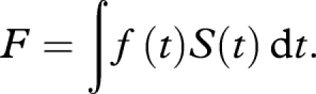This quantity is also known as net fecundity. A probable optimization target for fly populations evolving in new habitats is to maximize the total number of eggs produced, which corresponds to F; such optimization would target maximal population growth. It implies that age-specific reproductive schedules are evolving to track changes in the population survival schedule, thus optimizing reproductive fitness, while the survival schedule is influenced by the invaded habitat or is subject to genetic drift. Various forces which shape reproduction in wild insect populations have been identified in Rosenheim et al. (2008) and the references quoted there. Discussion of related optimization problems can be found in Vaupel et al. (2004) and Charnov et al. (2007).

Without further constraints, this optimization problem is ill-posed. Fast rising reproduction to deplete all eggs at a very young age, before rising hazard rates crimp any further reproduction owing to the death of the individual, would ensure maximum reproductive success. This is not observed in any of the cohorts, which means that either there are inherent physiological constraints to the speed in which reproduction can be ramped up, or that extended reproductive periods carry inherent benefits. Such benefits may derive from higher overall chances that the laid eggs lead to viable offspring when they are laid over an extended period of time, owing to stochasticity in the environment. Occasional negative environmental or seasonal influences of the habitat have only limited impact if egg-laying periods are extended, but can have serious negative effects if egg-laying occurs in a very brief period. If all egg-laying takes place in a very short interval and external conditions during that time are not conducive to the maturing of eggs and young flies, the entire batch of eggs laid by individual flies would be lost.

Environmental stochasticity coupled with short-term reproductive periods thus carries the risk of overall lower population net reproduction. Formally, assume the domain [0,T] of the lifespan of the flies can be divided into intervals I_j, j = 1, … , m, and the viability of the flies in the jth interval is described by an all-or-nothing random outcome characterized by a 0–1 random variable A_j, which we assume to be Bernoulli with probability p, for a value p with 0 < p < 1. Here, outcome A_j = 1 with probability p for a value 0 < p < 1 denotes viability of all eggs laid during the interval I_j, and outcome A_j = 0 with probability 1 − p denotes that none of the eggs laid in interval I_j is viable. We assume that the A_j are independently and identically distributed. In this situation, the fecundity F is a random outcome, depending on the periodic effects A_j that affect egg survival, and is given by

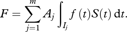Straightforward calculations then lead to

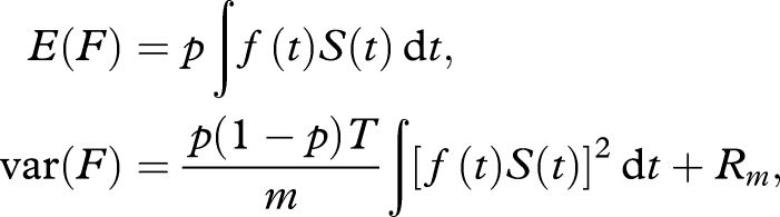where R_m denotes terms of smaller order o(1/m). For a given p, sharp increases in very early reproduction will therefore lead to larger values of var(F). Such increased volatility of egg-laying will lead to overall lower reproductive success in the face of stochastic environments. These conclusions are robust and also hold under alternative assumptions. The asymmetry of the risk makes it probable that evolutionary changes will trend towards optimizing fecundity F in concert with limiting var(F).

The tendency to minimize egg-laying volatility for the long-lived cohorts, for which survival only starts to decline strongly after 80 days, as evidenced by the hazard rate estimates given in Diamantidis et al. (2009), provides an additional explanation for the close association of reproduction and survival. Thus the reproductive adaptation hypothesis favours trends towards later and more drawn out reproductive schedules for the longer lived cohorts, in accordance with observations. Another noteworthy feature is that according to the data reported in Diamantidis et al. (2009), net fecundity F shows remarkably little variation across populations, while there is a tremendous variation in terms of population survival and individual reproductive trajectories. This is further evidence for the very effective co-regulation of survival and reproductive schedules across the populations considered in this study.

Many factors influence selection for shorter or longer lifespan, ranging from host availability and predation to seasonality and predictability. However, it is noteworthy that the three short-lived biotypes were all collected from tropical regions and the three longer lived biotypes were all collected from regions with Mediterranean-like climates. Inasmuch as lifespan evolutionary theory (Orzack 2003) supports the notion that selection favours longer lifespans in both uncertain environments or in environments with dearth periods of resource availability, the lifespans of the long-lived group of medfly biotypes may have evolved in response to host-free summer periods, owing to either chance or seasonal variation. Specific host plants and differences in their chemistry may play an important role in determining population longevity. For example, Coffea arabica serves as a host plant for the short-lived but not for the long-lived populations.

As our statistical analysis establishes association but not causality, various mechanisms could contribute to the observed close co-regulation between reproduction and longevity. For example, fertility trajectories themselves may have an effect on survival of individual flies (‘cost of reproduction’). It is possible that host plant availability leads to the evolution of early reproduction in a locally adapted population, with subsequent detrimental effects on lifespan (Kirkwood & Rose 1991). The observed survival schedules would then represent to some extent a consequence of the evolution of the shape of the reproductive schedules. However, the cost of reproduction effect, as far as it exists, is fairly weak, explaining at best a small fraction of the variance of age-at-death for individual flies, making this explanation of the observations less probable. The reproductive adaptation hypothesis, which states that different population survival schemes result in differences in reproductive trajectories, is supported by the fact that some degree of adaptation is a prerequisite for population survival, as well as the empirical observation that differences in population reproductive schedules nearly vanish when adjusting for different survival across populations. Our findings illustrate the usefulness of functional statistical methods and unequivocally demonstrate that the reproduction–survival relationship is tightly controlled across populations.

References

- Carey J. R., Harshman L. G., Liedo P., Müller H. G., Wang J. L., Zhang Z.2008Longevity–fertility trade-offs in the tephritid fruit fly, Anastrepha ludens, across dietary-restriction gradients. Aging Cell 7, 470–477 (doi:10.1111/j.1474-9726.2008.00389.x) [DOI] [PMC free article] [PubMed] [Google Scholar]
- Charnov E. L., Warne R., Moses M.2007Lifetime reproductive effort. Am. Nat. 170, E129–142 [DOI] [PubMed] [Google Scholar]
- Diamantidis A. D., Papadopoulos N., Nakas C. T., Wu S., Müller H. G., Carey J. R.2009Life history evolution in a globally-invading tephritid: patterns of survival and reproduction in medflies from six world regions. Biol. J. Linn. Soc. 97, 106–117 (doi:10.1111/j.1095-8312.2009.01178.x) [Google Scholar]
- Duyck P.-F., David P., Quilici S.2007Can more K-selected species be better invaders? A case study of fruit flies in La Reunion. Divers. Distrib. 13, 535–543 (doi:10.1111/j.1472-4642.2007.00360.x) [Google Scholar]
- Futuyma D. J.2005Evolution Sunderland, MA: Sinauer Associates, Inc [Google Scholar]
- Gomulkiewicz R., Kingsolver J.2007A fable of four functions. J. Evol. Biol. 20, 20–21 (doi:10.1111/j.1420-9101.2006.01231.x) [DOI] [PubMed] [Google Scholar]
- Hall P., Leng X., Müller H. G.2008Weighted-bootstrap alignment of explanatory variables. J. Stat. Plann. Inference 138, 1817–1827 (doi:10.1016/j.jspi.2007.06.032) [Google Scholar]
- Kirkpatrick M., Heckman N.1989A quantitative genetic model for growth, shape, reaction norms, and other infinite-dimensional characters. J. Math. Biol. 27, 429–450 (doi:10.1007/BF00290638) [DOI] [PubMed] [Google Scholar]
- Kirkwood T. B. L., Rose M. R.1991Evolution of senescence: late survival sacrificed for reproduction. Phil. Trans. R. Soc. Lond. B 332, 15–24 (doi:10.1098/rstb.1991.0028) [DOI] [PubMed] [Google Scholar]
- Lee C. E.2002Evolutionary genetics of invasive species. Trends Ecol. Evol. 17, 386–391 (doi:10.1016/S0169-5347(02)02554-5) [Google Scholar]
- Müller H. G., Carey J. R., Wu D., Liedo P., Vaupel J. W.2001Reproductive potential predicts longevity of female Mediterranean fruitflies. Proc. R. Soc. Lond. B 268, 445–450 (doi:10.1098/rspb.2000.1370) [DOI] [PMC free article] [PubMed] [Google Scholar]
- Orzack S. H.2003How and why do aging and lifespan evolve? Popul. Dev. Rev. (Suppl.) 29, 19–38 [Google Scholar]
- Partridge L., Harvey P. H.1985Evolutionary biology: cost of reproduction. Nature 316, 20 (doi:10.1038/316020a0) [Google Scholar]
- Ramsay J. O., Dalzell C. J.1991Some tools for functional data analysis (with discussions). J. R. Stat. Soc. Ser. B 53, 539–572 [Google Scholar]
- Ramsay J. O., Silverman B. W.2005Functional data analysis Springer Series in Statistics,2nd edn.New York, NY: Springer [Google Scholar]
- Rosenheim, Jay A., Jepsen S. J., Matthews C. B., Smith D. S., Rosenheim M. R.2008Time limitation, egg limitation, the cost of oviposition, and lifetime reproduction by an insect in nature. Am. Nat. 172, 486–496 [DOI] [PubMed] [Google Scholar]
- Tuljapurkar S.1982Population dynamics in variable environments. III. Evolutionary dynamics of r-selection. Theor. Popul. Biol. 21, 141–165 (doi:10.1016/0040-5809(82)90010-7) [Google Scholar]
- Tuljapurkar S., Horvitz C., Pascarella J.2003The many growth rates and elasticities of populations in random environments. Am. Nat. 162, 489–502 [DOI] [PubMed] [Google Scholar]
- Vaupel J. W., Baudisch A., Dölling M., Roach D. A., Gampe J.2004The case for negative senescence. Theor. Popul. Biol. 65, 339–351 [DOI] [PubMed] [Google Scholar]
- Yao F., Müller H. G., Wang J. L.2005Functional linear regression analysis for longitudinal data. Ann. Stat. 33, 2873–2903 (doi:10.1214/009053605000000660) [Google Scholar]