Spread of infectious disease through clustered populations

Abstract

Networks of person-to-person contacts form the substrate along which infectious diseases spread. Most network-based studies of this spread focus on the impact of variations in degree (the number of contacts an individual has). However, other effects such as clustering, variations in infectiousness or susceptibility, or variations in closeness of contacts may play a significant role. We develop analytic techniques to predict how these effects alter the growth rate, probability and size of epidemics, and validate the predictions with a realistic social network. We find that (for a given degree distribution and average transmissibility) clustering is the dominant factor controlling the growth rate, heterogeneity in infectiousness is the dominant factor controlling the probability of an epidemic and heterogeneity in susceptibility is the dominant factor controlling the size of an epidemic. Edge weights (measuring closeness or duration of contacts) have impact only if correlations exist between different edges. Combined, these effects can play a minor role in reinforcing one another, with the impact of clustering the largest when the population is maximally heterogeneous or if the closer contacts are also strongly clustered. Our most significant contribution is a systematic way to address clustering in infectious disease models, and our results have a number of implications for the design of interventions.

1. Introduction

Recently, H5N1 avian influenza and SARS have raised the profile of emerging infectious diseases. Both can infect humans, but have a primary animal host. Typically, such zoonotic diseases emerge periodically into the human population and disappear (e.g. Ebola, hantavirus, rabies), but sometimes (e.g. HIV) the disease achieves sustained person-to-person spread. With the advent of modern transportation networks, diseases that formerly emerged in isolated villages and died out without further spread may now spread worldwide.

A number of interventions are available to control emerging diseases, each with distinct costs and benefits. To design optimal policies, we must address several related, but nevertheless distinct, questions. How fast would an epidemic spread? How likely is a single introduced infection to result in an epidemic? How many people would an epidemic infect? We quantify these using ₀, the basic reproductive ratio, which measures the average number of new cases each infection causes early in the outbreak; , the probability that a single infection sparks an epidemic; and , the attack rate or fraction of the population infected in an epidemic. Understanding these different quantities and what affects them helps us to select policies with maximal impact for given cost.

Many different models are used to study disease spread. Perhaps the most important decision in developing a model is how the interactions of the population are represented. Owing to the complexity of the population, it is invariably necessary to make simplifying assumptions. The errors (and therefore the conclusions) resulting from many of these approximations are not well quantified. In this paper, we will focus on quantifying the impact of clustering (the tendency to interact in small groups) and individual-scale heterogeneity on the spread of an epidemic.

Based on how they handle clustering, models for population structure fit into a hierarchy of three classes (which in turn may be subdivided). At the simplest level, the population is assumed to mix without any clustering. Most existing models fall into this category. At the most complex level, agent-based models are used: the movements of each individual are tracked and people who are in the same location are able to infect one another. These models typically require significant resources to develop, and the clustering is explicitly included. An intermediate level of complexity attempts to introduce the clustering as a parameter (or several parameters). Usually these models consider clustering only in terms of the number of triangles in a network, but as we shall see, other structures may play a role.

Before introducing the details of our model, we review some previous work. All the models we consider are susceptible–infected–recovered (SIR) epidemic models (Anderson & May 1991), in which individuals begin susceptible, become infected by contacting infected individuals and finally recover with immunity.

For unclustered populations, ordinary differential equation (ODE) models were among the earliest models used (Kermack & McKendrick 1927) and remain the most common. They are deterministic, and so cannot directly calculate , but they give insights into the factors controlling ₀ and . Because they assume mass-action mixing, it is difficult to incorporate individual heterogeneity in the number of contacts. More recently, some network-based models have been introduced for unclustered populations (Andersson 1998; Newman 2002; Meyers et al. 2005, 2006; Kenah & Robins 2007; Miller 2007; Meyers 2007). These models represent the population as nodes with edges between nodes representing contacts, along which disease spreads stochastically. Heterogeneity in the number of contacts is introduced by modifying the degree (number of edges) of each node. By neglecting clustering, these studies are able to make analytic predictions through branching process arguments. A recent sociological study (Mossong et al. 2008) has used surveys with participants recording the length and nature of their contacts. These data are valuable for providing the contact distribution needed for the above network models, and allow us to apply network results to real populations. However, these data do not directly tell us anything about the clustering of the population resulting from family/work/other groups. Other recent work by Kenah & Robins (2007) and Miller (2007) analytically addresses the impact of heterogeneity in infectiousness and susceptibility in unclustered networks.

Using agent-based simulations (Eubank et al. 2004; Barrett et al. 2005; Ferguson et al. 2005; Del Valle et al. 2006; Germann et al. 2006; Ajelli & Merler 2008) allows us to directly incorporate clustering. In these simulations, the population is a collection of individuals who move and contact one another. The modeller has complete control over the parameters governing interactions and how the disease spreads. This allows us to study many effects, but introduces many parameters. It is difficult to test the accuracy of the assumptions used to generate these models and to extract which parameters are essential to the disease dynamics. The expense of developing these simulations is frequently prohibitive.

In this paper, we introduce a systematic approach for calculating the impact of clustering and quantifying the error. Because our model investigates disease spread in clustered networks, we provide a more detailed review of previous work on clustering and disease. A few investigations have been made into the interaction of clustering with disease spread using network models. The attempts that have been made (Keeling 1999; Newman 2003a; Serrano & Boguñá 2006a,b; Britton et al. 2007; Eames 2008) typically use approximations whose errors are not quantified, resulting in apparently contradictory results. A few papers (Kuulasmaa 1982; Trapman 2007; Miller 2008) have considered clustering and heterogeneities, rigorously showing that increased heterogeneity tends to decrease and , but without quantitative predictions. Recently, Eames (2008) has considered the spread of epidemics in a class of random networks for which the number of triangles could be controlled. It may be inferred from his fig. 3 that clustering decreases the growth rate and that sufficient clustering can increase the epidemic threshold. However, at small and moderate levels, clustering appears not to alter the final size of epidemics significantly. Similar observations have been made by Bansal (2008). At first glance, this contradicts the observations of Serrano & Boguñá (2006a,b) that clustering significantly reduces the size of epidemics, but that sufficiently strong clustering reduces the epidemic threshold (see also Newman 2003a), allowing epidemics at lower transmissibility. The discrepancy in epidemic size may be resolved by noting that the networks in Serrano & Boguñá (2006a,b) have low average degree. We will see that clustering affects the size only if the typical degree is small or clustering is very high. The apparent discrepancy in epidemic threshold with strong clustering may be resolved by noting that the form of strong clustering considered by Serrano & Boguñá (2006a,b) forces preferential contacts between high-degree nodes. The reduction in epidemic threshold is perhaps better understood in terms of degree–degree correlations than in terms of clustering.

Figure 3.

Different options for paths of length 2 between nodes u and v: (a) n_uv=4, x_uv=1; (b) n_uv=4, x_uv=0.

In this paper, we develop techniques to incorporate general small-scale structure (beyond triangles) into the calculations of ₀, and . To calculate ₀, we develop a systematic series expansion that allows us to interpolate between unclustered and clustered results by including more terms. To calculate and , we use a similar approach, but give only the estimates on the size of correction terms. Our methods give us a rigorous means to understand how the unclustered results relate to more realistic populations, and our results resolve the apparent discrepancies mentioned above. Our theory accurately predicts epidemic behaviour in a more realistic contact network derived from an agent-based simulation of Portland, Oregon, by EpiSimS (Del Valle et al. 2006). We expand this to investigate the interplay of clustering, heterogeneities in individual infectiousness or susceptibility, and variations in edge weights in their effects on ₀, and .

The paper is organized as follows: §2 describes our model and networks and summarizes earlier work on unclustered networks. These results will be the leading-order terms for our expansions for clustered networks in the remainder of the paper. Section 3 considers how epidemics spread in a clustered network assuming homogeneous transmission. We derive the corrections to ₀ and show that the corrections to and are insignificant unless the typical degree is small or clustering very high. Section 4 considers epidemics in clustered networks with heterogeneous infectiousness or susceptibility, building on §3. Section 5 extends this further to consider epidemics spreading on clustered networks with weighted edges. Edges with large weights tend to occur in family or work groups, which magnifies the impact of clustering. Finally, §6 discusses the implications of our results, particularly for designing interventions. We conclude that, in general, heterogeneity significantly impacts and , but not ₀, while clustering impacts ₀ significantly, but not and . Heterogeneity or edge weights may enhance the impact of clustering.

2. Formulation

2.1. The disease model

We consider the spread of a disease using a discrete SIR model on a static network G. Nodes of G represent individuals and edges represent (potentially infectious) contacts. The contact structure of the network is fixed during the course of the outbreak. The degree k of a node u is the number of edges containing u. Figure 1 shows a sample outbreak. For a single infection, the index case is chosen uniformly from the population to begin an outbreak. Infection spreads along an edge from an infected node u to a susceptible node v with probability T_uv, the transmissibility. The time it takes for infection and recovery to occur may vary but does not affect our results. Once u recovers it cannot be reinfected. Typically, for a large random network with a population of N=|G| nodes, the final size of outbreaks is either large, with (N) cumulative infections, or small, with (log N) infections (Bollobás 2001). Large outbreaks are epidemics and small outbreaks are non-epidemics.

Figure 1.

A sample network and several stages of an outbreak. Nodes begin susceptible (small circles), become infected (large open circles), possibly infecting others along edges, and then recover (large filled circles). The outbreak finishes when no infected nodes remain.

2.1.1. Transmissibility

A number of factors influence the transmissibility from u to v such as the viral load and duration of infection of u, the vaccination history and general health of v, the duration and nature of the contact between u and v and characteristics of the disease.

For each node u, we denote its ability to infect others by _u and its ability to be infected by _u. Each edge has a weight w_uv. The parameter α measures disease-specific quantities. In most of our calculations, we assume that these are scalars and follow Del Valle et al. (2007) and Miller (2007), setting

2.1

If all contacts are identical, w_uv may be absorbed into α

2.2

Note that T_uv is a number assigned to an edge, while is a function that states what the transmissibility between two nodes would be if they shared an edge.

With mild abuse of notation, we denote the probability density functions (pdfs) of , and w by P(), P() and P(w), respectively. We assign and independently, but allow w to be assigned either independently or based on observed contacts (i.e. by observing contacts in a population, we may create a static network with edge weights assigned based on the observed contact). If w is assigned independently, then it is possible to eliminate edge weights from the analysis by marginalizing over the distribution of weights. However, if weights are not independent (for example work or family contacts tend to have correlated weights), then the details of the distribution and the correlations are important.

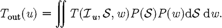
Given the infectiousness _u of node u, we follow Miller (2007, 2008) and define its out-transmissibility

2.3

This is the marginalized probability that u infects a randomly chosen neighbour given _u. From the definition of T_out and the pdf P(), we can calculate the pdf Q_out(T_out). We symmetrically define the in-transmissibility T_in and its pdf Q_in(T_in).

We denote the average of a quantity by 〈.〉. The average transmissibility 〈T〉 is

2.4

2.1.2. Epidemic percolation networks

Rather than studying outbreaks as dynamic processes on networks, we may consider them in the context of epidemic percolation networks (EPNs; Kenah & Robins 2007a,b; Miller 2008). The EPN framework allows us to study epidemics as static objects and is useful for quickly estimating ₀, and . In this section, we summarize properties of EPNs; more details are provided in Kenah & Robins (2007), Miller (2007, 2008) and in §A of the electronic supplementary material.

Once the properties of the nodes and edges are assigned, an EPN is created as follows: we place each node of G into . For each edge {u,v} in G, we place directed edges (u,v) and (v,u) into independently with probability T_uv and T_vu, respectively. The nodes infected in an outbreak correspond exactly to those nodes that may be reached from the index case following the edges of . More specifically, the distribution of out-components of a node u in different EPN realizations matches the distribution of outbreaks resulting from different epidemic realizations in the original model with u as the index case. It may be shown that the distributions of out- and in-component sizes give us information about the probability of nodes to start an epidemic or become infected in an epidemic. We will see that in a large population the structure of a single EPN can be used to accurately estimate ₀, and .

Once we create an EPN and choose the index case, we define the rank of node v as the length of the shortest directed path from the index case to v.1 If no such path exists, v is never infected.

Interchanging all arrow directions interchanges and . This means that if we can calculate , then may be calculated by the same technique, but with the direction of infection reversed. Owing to this, we focus our attention on calculating and apply the same methodology to calculate . An important consequence is that if T is constant, then = (Newman 2002; Miller 2007).

2.1.3. The basic reproductive ratio

We expect that epidemics are possible if and only if the basic reproductive ratio ₀ is greater than 1. That is, if an average infection causes more than one new case, an epidemic may occur, but otherwise the outbreak dies out quickly. However, this use of ₀ is not consistent with the typical definition: the average number of new infections caused by a single infected individual introduced into a fully susceptible population, which gives . A more appropriate definition is the average number of new infections caused by infected individuals early in outbreaks. The distinction is subtle, but results from the fact that whether an outbreak can grow depends on whether the people of low rank infect more than one person each (Diekmann et al. 1990). Low-rank individuals may be different from the average individual. Most obviously, they have more contacts (Feld 1991; Newman 2002); but with clustering, they also have a disproportionately large fraction of neighbours infected or recovered.

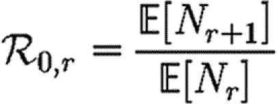
In order to quantify ₀ more rigorously, we first define N_r to be the number of people of rank r for a given outbreak simulation. We then define the rank reproductive ratio

2.5

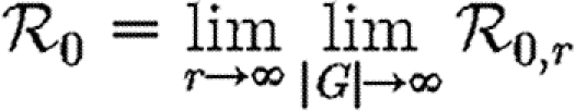
to be the expected number of new cases caused by a rank r node (averaged over all possible outbreak realizations). corresponds to the usual definition of ₀. In practice, we find that _0,r reaches a plateau quickly as r increases before eventually decreasing as the finite size of the population becomes important. Consequently, an improved definition of ₀ is the limit of _0,r as r grows, subject to the assumption that _0,r is unaffected by the finite size of G. This gives (cf. Trapman 2007)

2.6

and generalizes the definition given by Diekmann et al. (1990) for ODE models. Under this definition, epidemics are possible if ₀>1, but not if ₀<1. We discuss this further in §B of the electronic supplementary material. In a large population, considering multiple index cases with a single EPN gives a good estimate of and hence _0,r.

2.2. Configuration model networks

We consider two different types of networks. The first is a class of (unclustered) random networks for which we can derive analytic results based only on the degree distribution. These analytic results will form the leading-order term of our perturbation expansions. The second is a more complicated network resulting from an agent-based simulation, which we will use to demonstrate the accuracy of our perturbation expansions.

Our random networks are created by an algorithm that has been discovered independently a number of times (e.g. Molloy & Reed 1995). These have come to be called configuration model (CM; Newman 2003b) networks. These networks are maximally random given the degree distribution. As the number of nodes in a CM network grows, the frequency of short cycles becomes negligible. The resulting lack of clustering allows us to calculate analytic results for epidemics. We briefly discuss these results assuming T is constant. More details are in Andersson (1998), Newman (2002), Meyers et al. (2006), Kenah & Robins (2007), Marder (2007), Miller (2007) and Noël et al. (2009) and §C of the electronic supplementary material (which also addresses edge weights).

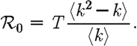
In the early stages of an outbreak in a CM network, the probability that a newly infected (non-index case) node has degree k is kP(k)/〈k〉. Clustering is unimportant and so the node will have k−1 susceptible neighbours, regardless of its rank. Thus, the expected number of infections caused by a newly infected node is

2.7

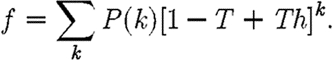
To calculate the probability that infection of a randomly chosen index case results in an epidemic, we instead calculate the probability f=1− that it does not. Then f is the probability that each neighbour of the index case is either not infected, or infected but does not start an epidemic. Defining h to be the probability that a secondary case does not start an epidemic,

2.8

We find a similar relationship for h, except that the probability for a secondary case to have degree k is kP(k)/〈k〉 and only k−1 neighbours are susceptible

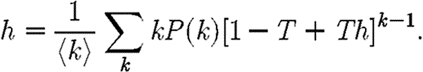2.9

We solve this recurrence relationship for h numerically, and use the result to find f. follows immediately. Because T is constant, this also gives (Newman 2002; Miller 2007).

If T is not constant, the calculation becomes more difficult, and is discussed further in §C of the electronic supplementary material and Kenah & Robins (2007) and Miller (2007). In general, if T can vary for CM networks, 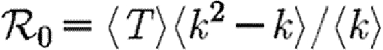, while the values calculated assuming constant T give upper bounds for and .

2.3. The EpiSimS network

We are interested in understanding the impact of clustering on disease spread. The term clustering is rather vague, and is usually measured by the number of triangles in a network (Watts & Strogatz 1998). However, any sufficiently short cycles impact the spread of an infectious disease. For our purposes, we think of a clustered network as a network with enough short cycles to impact disease dynamics.

It is relatively simple to measure the degree distribution of a population using survey methods. We can easily calculate ₀, and for a CM network with the same degree distribution, but the errors between these values and the values for the original clustered network are unknown. Our goal in this paper is to develop analytical techniques to quantify these errors.

To test our predictions, we turn to an agent-based network derived from a single EpiSimS (Eubank et al. 2004; Barrett et al. 2005; Del Valle et al. 2006) simulation of Portland, Oregon. The simulation includes roads, buildings and a statistically accurate (based on census data) population of approximately 1.6 million people who perform daily tasks based on population surveys. This gives a highly detailed knowledge of the interactions in the synthetic population. The degree distribution and contact structure emerge from the simulation. The resulting network has significant clustering and average degree of approximately 16. More details are in §D of the electronic supplementary material.

3. Clustered networks with homogeneous nodes

In this section, we assume that the population is homogeneous and all contacts are equally weighted. Consequently, transmissibility is constant: for all edges. It follows that = (Newman 2002; Miller 2007). We develop a predictive theory for ₀, and and test the theory with simulations on the EpiSimS network. We begin with ₀.

3.1. The basic reproductive ratio

The simulated rank reproductive ratio _0,r is shown in figure 2 for 0≤r≤4. At all values of T, 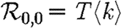is clearly distinct from _0,r, r>0 (which are close together). For r>0, _0,r is asymptotic to the unclustered approximation T〈k²−k〉/〈k〉 as T→0. This is because at small T the disease only rarely follows all edges of short cycles and so clustering has no impact. As T increases, these curves lie significantly below the unclustered approximation, because clustering reduces the number of available susceptibles. _0,4 peels away from _0,1, _0,2 and _0,3 for larger T because the population is finite, and so the number of susceptibles available to infect after rank 4 is reduced. In larger populations, _0,4 would not deviate.

Figure 2.

(a,b) Simulated values of the rank reproductive ratio 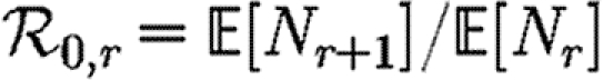for r=0, …, 4 using an EPN from the (fixed) EpiSimS network with a homogeneous population, compared with the unclustered prediction. (b) At small T, _0,1–_0,4 match the unclustered prediction (black solid curve, unclustered ₀ prediction; black dashed curve, _0,0; grey solid curve, _0,1; dotted curve, _0,2; dot-dashed curve, _0,3; grey dashed curve, _0,4). Each data point for 〈T〉≤0.5 is for 10⁵ index cases in a single EPN, while each data point for T>0.5 is for 10³ index cases. Noise becomes less significant at larger r.

We conclude that _0,r converges quickly, and that _0,1 is a good approximation to ₀, but _0,0 is not. This implies that the network has an important structure contained in the paths of length 2, but not in the paths of length 3. This fortunate observation allows us to approximate ₀ by _0,1, which we may analytically calculate with relative ease (_0,r becomes combinatorially hard as r grows). To find , we first note that . 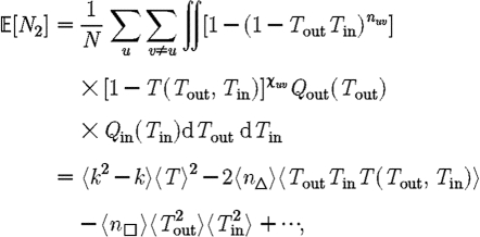Calculating is more difficult: consider all pairs of nodes u and v with at least one path of length 2 between them. Let n_uv be the number of paths of length 2 between u and v and Χ_uv be an indicator function: Χ_uv=1 if {u,v} is an edge and Χ_uv=0 if it is not (figure 3). The probability that an infection of u results in infection of v in exactly two steps is 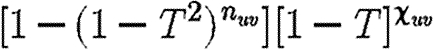. Summing this over all pairs yields (where N is the size of the population and each pair u and v appears twice)

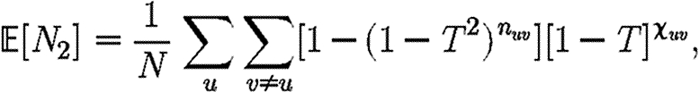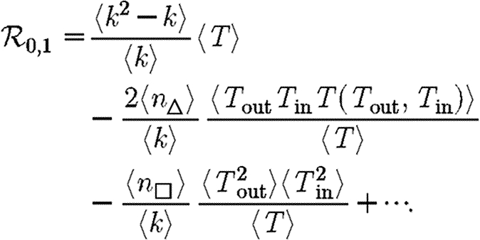
which allows us to calculate _0,1 exactly. This sum is straightforward to calculate, but we can increase our understanding with a small T expansion. We approximate for T≪1 by

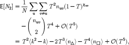where is the average number of triangles each node is in, and 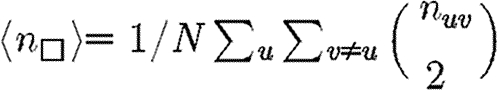is the average number of squares each node is in (cf. Hastings 2006). Higher order terms involve more complicated shapes. This gives

3.1

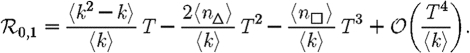
At the leading order, we recover the unclustered prediction for ₀, reflecting the fact that at small T the probability the outbreak follows all edges of a cycle is negligible. As T increases, the first corrections are due to triangles, then squares, then pairs of triangles sharing an edge and sequentially larger and larger structures made up of paths of length 2. A comparison of these approximations with the exact value is shown in figure 4.

Figure 4.

(a,b) Comparison of first three asymptotic approximations for _0,1 from equation (3.1) with the exact value for the EpiSimS network. (b) The comparison at small T is shown (solid curve, exact _0,1; dotted curve, first approximation; dot-dashed curve, second approximation; dashed curve, third approximation).

Although we have defined ₀ for an ensemble of realizations, figure 5 shows that _0,1 accurately predicts the observed ratio N_r+1/N_r for individual simulations once the outbreaks are well established. Early in outbreaks, the behaviour is dominated by stochastic effects, and so the ratio of successive rank sizes is noisy. Once the outbreak has grown large enough, random events become unimportant and the ratio settles at _0,1.2

Figure 5.

The progression of 10 simulated epidemics for (a) T=0.1 and (b) T=0.2 in the EpiSimS network. (a) N_r+1/N_r against rank and (b) the cumulative fraction of the population infected are shown (dotted curve, unclustered ₀ prediction; dashed curve, _0,1).

3.2. Epidemic probability and size

In order to assess the effect of clustering on and , we compare epidemics on the EpiSimS network with the analytic predictions derived assuming a CM network of the same degree distribution in figure 6. The epidemic threshold is not notably altered, and the values of and are almost indistinguishable from the predictions made assuming no clustering, despite the large amount of clustering in the network.

Figure 6.

Probability and attack rate of epidemics for the (clustered) EpiSimS network (pluses) versus T, compared with the prediction derived from the degree distribution assuming no clustering. Each data point is from a single EPN (the variation in resulting from different EPNs is negligible).

Although initially surprising, these results may be understood intuitively as follows: if T is large enough that the disease follows all edges of a short cycle, then some other edge from a node of that cycle is likely to start an epidemic and the cycle does not prevent an epidemic. On the other hand, if T is smaller so that it does not follow all edges of a cycle, then the disease never sees the existence of the cycle, and the outbreak progresses as if there were no cycle.

To make this more rigorous, we first look at the epidemic threshold. We assume that ₀ is well approximated by _0,1. Let T₀=〈k〉/〈k²−k〉 be the threshold without clustering and T₀+δT be the threshold found by including the correction due to triangles. From equation (3.1), it follows that

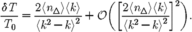3.2

Because a given node of degree k is contained in at most (k²−k)/2 triangles, we conclude 2〈n_△〉/〈k²−k〉≤1. So if 〈k〉/〈k²−k〉 is small, then the leading-order term of equation (3.2) is small and triangles do not significantly alter the epidemic threshold regardless of the density of triangles. For the EpiSimS network, 〈k〉/〈k²−k〉 takes the value 0.046, and so we do not anticipate clustering to play an important role in determining the threshold.

Above threshold, we assume that may be expanded much as (3.1)

3.3

where ₀ is the epidemic probability in a CM network of the same degree distribution. Although calculating _0,1 only requires information about the nodes of distance at most two from the index case, may depend on the effects occurring at larger distance, and so the expansion has many additional terms. In general, we expect that if the average degree is large, then the various coefficients of the correction terms are all small. The larger a structure is, the smaller we expect its corresponding coefficient to be. The coefficient for triangles ₁ may be found by

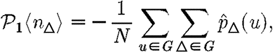where is the probability that a given triangle prevents an epidemic if u is the index case (regardless of whether u is part of the triangle). Reversing the order of summation, we get

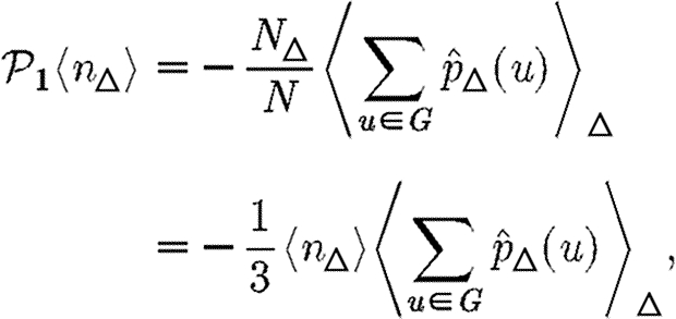where N_△ is the number of triangles in G and 〈.〉_△ is the average of the given quantity taken over all triangles. Thus

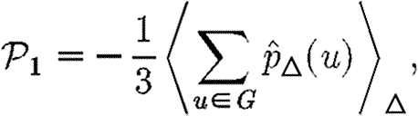and we can find ₁ by considering the average effect of a single triangle in an unclustered network.

To calculate the impact of a triangle with nodes u, v and w on for a given network, we consider that triangle and a randomly chosen edge {x,y} elsewhere in the network. If we replace the edges {v,w} and {x,y} with {v,x} and {w,y}, then we have a new network without the triangle, but with the same degree distribution. We must estimate the expected change in caused by switching the edges.

We begin by assuming that u is the index case. The triangle can affect only if the infection tries to cross all three edges, that is if the infection process ‘loses’ an edge because of clustering. This may happen in three distinct ways. In the first, node u infects both v and w, and then v and/or w tries to infect the other. In the second, u infects v but not w, then v infects w and finally w tries to infect u. The third is symmetric to the second (with u infecting w).

To leading order we can ignore other short cycles, so the probability that an edge leading out of u (not to v or w) will not cause an epidemic is g=1−T+Th, where h (as before) is the probability that a randomly chosen secondary case does not cause an epidemic in an unclustered network and can be calculated using equation (2.9).

We perform a sample calculation with the first case: u infects both v and w. Assume that u has degree k_u, v has degree k_v and w has degree k_w. The probability that u infects both v and w without some other edge leading from u, v or w starting an epidemic is . If the {v,w} edge were broken and v and w were joined to x and y, respectively (figure 7), then the new probability of u to infect both v and w without an epidemic becomes . The difference is , which is the product of three terms, all at most 1. If the sum k_u+k_v+k_w is moderately large, then either or (if g is not close to 1 then the first term is small, otherwise the second term is small). Thus, the triangle has little impact on the epidemic probability in this case.3 Similar analysis applies to the other two cases where the w to u or v to u infections are lost. Provided the typical sum of degrees of nodes in a triangle is relatively large, the probability of an epidemic when the index case is in the triangle is not impacted significantly.

Figure 7.

Replacing the edges {v,w} and {x,y} with {v,x} and {w,y} breaks the triangle and allows more infections, without affecting the degree distribution.

If the index case is not part of the triangle, then the above analysis is modified because we must also consider each node in the path from the index case to the triangle. We must first calculate the probability that infection reaches a node in the triangle while simultaneously no intermediate node sparks an epidemic, and then we calculate the probability as above that the triangle prevents an epidemic. If the index case is u₁ and the path from u₁ to the triangle goes through u₂, …, u_n and then reaches u, then the probability that the triangle prevents an epidemic is given by 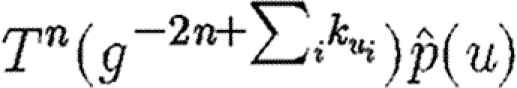. This falls off very quickly, and so nodes not in the triangle are unimportant, unless typical degrees are small.

By contrast, in a network with small average degree and a significant number of triangles, this becomes significant. This explains the observations of Serrano & Boguñá (2006a,b) who use networks with average degree less than 3 and find that clustering significantly alters .

It is tempting to generalize our conclusion and state that if the average degree is large, clustering has no impact on or . However, there are a number of counter-examples: consider a network made up of isolated cliques with N_c nodes, then in expansion (3.3), the coefficient for cliques of N_c nodes will not be small. Consequently, care must be taken when using such an expansion to ensure that neglected terms resulting from larger scale structures are in fact negligible. For social networks, we generally anticipate this highly segregated situation to be unimportant.

We conclude that for most reasonable networks, clustering is only important for and if the typical degrees of nodes are low in which case ₀ is small. A consequence of these results is that if ₀ is moderately large, then and are effectively unaltered by clustering. If ₀ is small, however, clustering may or may not play a role in determining and , depending on whether ₀ is small because the degrees are small or T is small.

4. Clustered networks with heterogeneous nodes

When we drop the assumption of constant transmissibility, disease spread becomes more complicated. If is heterogeneous and u infects a neighbour, then the a posteriori expectation for T_out(u) becomes higher: it is likely to infect more neighbours. This accentuates the effect of short cycles, enhancing the impact of clustering on ₀, and . A similar argument applies with heterogeneity in : if v is not infected by one of its neighbours, then the a posteriori expectation for T_in(v) becomes lower: it is less likely to be infected by other neighbours, and so has multiple opportunities to prevent an epidemic. Again this accentuates the effect of short cycles.

In this section, we investigate how varying the infectiousness and susceptibility of nodes in the EpiSimS network enables clustering to alter the values of ₀, and . We will make use of the ordering assumption and its consequences from Miller (2008): if u₁ is ‘more infectious’ than u₂ in a given instance (or v₁ ‘more susceptible’ than v₂), then u₁ is always more infectious than u₂ (or v₁ always more susceptible than v₂). More specifically, the ordering assumption states that T_out(u₁)>T_out(u₂) if and only if 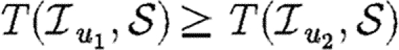for all , with inequality for some , and the corresponding statement for T_in. The results of Miller (2008) show that if the ordering assumption holds, heterogeneity tends to reduce and , and the upper bounds on and correspond to homogeneous populations (constant T).

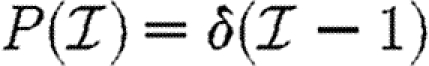
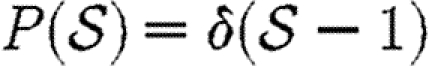
For simulations in this section, we consider five different illustrative cases, which will be denoted throughout by the symbols given in table 1. In the first four cases, we use equation (2.2), so that 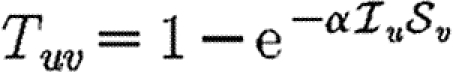with the distribution of and varying for each. We vary α to change the average transmissibility. In the fifth case, the out-transmissibility is maximally heterogeneous: a fraction 〈T〉 of the population infect all neighbours, while the remaining 1−〈T〉 infect no neighbours.

Table 1.

For the calculations of §§4 and 5, we determine T_uv using equations (2.1) and (2.2) with the distributions of and given in the first four rows, or by considering a maximally heterogeneous population for which 〈T〉 of the population infects all neighbours and 1−〈T〉 infects no neighbours. (The function δ is the Dirac delta function.)

symbol	infectiousness	susceptibility
	maximally heterogeneous	homogeneous Tin=〈T〉

The fifth case gives a lower bound on for a homogeneously susceptible population (Trapman 2007). It is hypothesized to remain a lower bound on if susceptibility is allowed to vary (Miller 2008). We could also consider maximal heterogeneity in susceptibility, but the results for and merely correspond to interchanging their values for maximal heterogeneity in infectiousness, and so we do not need to consider it explicitly.

4.1. The basic reproductive ratio

We use simulations to calculate the rank reproductive ratio _0,r for the cases of table 1 and plot the result for 0≤r≤4 in figure 8. Note that _0,1 remains a good approximation to ₀. In the first four cases, ₀ is again asymptotic to the unclustered approximation as 〈T〉→0. There are small kinks for and at 〈T〉=0.5 and 〈T〉=0.7, respectively, resulting from the nature of those distributions. The heterogeneities act to enhance the effect of clustering on ₀, but the effect is relatively small.

Figure 8.

(a–e) calculated from EPNs for the heterogeneous examples of table 1 (black solid curve, unclustered ₀; black dashed curve, _0,0; grey solid curve, _0,1; dotted curve, _0,2; dot-dashed curve, _0,3; grey dashed curve, _0,4). (f) _0,1 values for all of the different cases, including both unclustered ₀ (solid curve) and homogeneous _0,1 (dotted curve) are compared.

In the final, maximally heterogeneous case , _0,1 remains a good approximation to ₀. At small values of 〈T〉, the heterogeneity causes clustering to have a larger impact than in a homogeneous population as seen in figure 8f, and so this is not asymptotic to the unclustered approximation. At larger values of 〈T〉, the heterogeneous and homogeneous growth rates are similar.

As before, we can calculate _0,1 analytically, which helps to explain our observations. If the ordering assumption holds, we may use a simplified notation T(T_out,T_in) to denote the transmissibility from a node with out-transmissibility T_out to a node with in-transmissibility T_in.4 We have 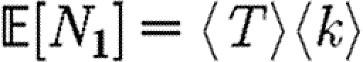and

and so we may express the growth rate as a perturbation about the unclustered case giving

4.1

For the second term, it may be shown that 〈T〉³≤〈T_outT_inT(T_out,T_in)〉≤〈T〉². The minimum occurs when T is constant, suggesting that the maximum growth rate occurs in a homogeneous population. The maximum 〈T〉² occurs either for

4.2

i.e. when the out-transmissibility is maximally heterogeneous, or when the in-transmissibility is maximally heterogeneous

4.3

Consequently, we expect that for given 〈T〉, the minimum growth rate occurs with maximally heterogeneous infectiousness or susceptibility. These two minima for _0,1 have previously been hypothesized to give lower bounds on and , respectively (Miller 2008).

We note that in the maximally heterogeneous case, the correction term in (4.1) is significant at the leading order in T. Consequently, if 〈n_△〉 is comparable with 〈k²−k〉/2 (i.e. the clustering coefficient (Watts & Strogatz 1998) is comparable with 1), then the threshold value of 〈T〉 may be increased by clustering, and ₀ is not asymptotic to the unclustered prediction as 〈T〉→0.

4.2. Probability and size

Figure 9 shows that the unclustered predictions provide a good estimate of and in the clustered EpiSimS network. We expect that in a network with sufficiently large average degree, the impact of clustering should once again be small.

Figure 9.

Comparison of (a) and (b) observed from EPNs in the clustered EpiSimS network with heterogeneities (symbols) with that predicted by the unclustered theory (curves) using table 1. Each data point is based on a single EPN. For both and , T_in(v)=〈T〉 for all nodes, and so the unclustered prediction for is the same.

We use arguments similar to that before, taking a triangle with nodes u, v and w. The reasoning becomes more difficult because knowledge that u infects v increases the expectation that u infects w. Consequently, the lost edges in triangles are more frequently encountered by the outbreak. However, the knowledge that u infects v also increases the expectation that u infects its other neighbours. For a triangle to prevent an epidemic, we need both that no edge outside the triangle leads to an epidemic and that the lost edge would otherwise have caused an epidemic. If the typical degree of the network is not small, then the fact that the lost edge is encountered more frequently may be offset by the fact that when it is encountered, other edges are more likely to spark an epidemic.

For where nodes infect all or none of their neighbours, the effect of different triangles that share the index case cannot be separated easily. The probability that the index case directly infects a set of m nodes of interest is 〈T〉, rather than T^m. Thus, expansions as in (3.3) do not work as well: terms that were previously higher order become significant. Close to the epidemic threshold, this can play an important role. However, well above the epidemic threshold, if the index case infects all of its neighbours, then an epidemic is almost guaranteed and so regardless of whether the network is clustered. Thus for , clustering affects only close to the epidemic threshold.

In the opposite case where nodes would be infected by any neighbour or else no neighbour, the values of and are interchanged. Thus, for maximally heterogeneous susceptibility, could be significantly altered close to the threshold. The reason for this is as follows: for the first step, the spread is indistinguishable from that of an outbreak with constant T. However, when infections of rank 1 attempt to infect their neighbours, they cannot infect any of the neighbours of the index case. By contrast, in the constant T case, any neighbour not infected by the index case would be susceptible at later steps. Consequently, the impact of triangles becomes much more important (by a factor of 1/〈T〉) and our earlier argument for neglecting them fails. The interaction of maximal heterogeneity with clustering in this case is larger, but it nevertheless becomes unimportant far from the threshold.

Our prediction that heterogeneity allows clustering to be more significant close to the threshold is borne out for where there is relatively strong heterogeneity in susceptibility just above the epidemic threshold. The epidemic threshold for is increased compared with the other cases. By contrast, there is much stronger heterogeneity in susceptibility for at 〈T〉=0.5 and in infectiousness for at 〈T〉=0.7. This results in a reduction in and , respectively, but because it is far from threshold, there is little deviation from the unclustered predictions.

5. Clustered networks with weighted edges

When we allow edges to be weighted, new complications arise. The weights we use in our simulations are the durations of contacts from the EpiSimS simulation and are discussed in more detail in §D of the electronic supplementary material. If a contact in the original EpiSimS simulation is longer, then a higher weight is assigned. If the weights of different edges were independent, then we could simply take . However, edge weights are not independent: clustered connections tend to have larger weights. If brief contacts are negligible, then the disease spreads on a subnetwork of the original network. The new network has a comparable number of short cycles to the original, but lower typical degree. This should enhance the impact of clustering.

For our calculations in this section, we first isolate the impact of weighted edges by taking a homogeneous population (==1) and using . We vary α in order to set 〈T〉. We then investigate a heterogeneous population using equation (2.1) with the first four distributions of table 1.

Results for a homogeneous population are shown in figure 10. Because T_uv=T_vu for all pairs, it follows that =. If different edge weights were uncorrelated, then the value of ₀ would match with figure 2 and and would match with figure 6. We see, however, that ₀ is significantly reduced from the homogeneous unweighted population (but _0,1 remains a good approximation). and are mildly reduced close to the threshold. These observations are consistent with our expectation that clustering should be accentuated by incorporating edge weights. Although the predictions for and are not far off, we expect that they would improve if we adjusted the degree distribution to match that of the effective network on which the disease spreads.

Figure 10.

(a) _0,r (black solid curve, unclustered ₀; black dashed curve, _0,0; grey solid curve, _0,1; dotted curve, _0,2; dot-dashed curve, _0,3; grey dashed curve, _0,4) and (b) and for the weighted EpiSimS network with a homogeneous population.

When the population is moderately heterogeneous (figure 11), we still find that _0,1 is a reasonable approximation to the true value of ₀; however, it slightly underestimates ₀ as 〈T〉 grows. Unfortunately, the analytic calculation of _0,1 is much more difficult, and so it is more appropriate to use simulations to estimate its value. If there were no correlation between weights of different edges, then the calculation would reduce to that of §4.

Figure 11.

(a–d) _0,r with heterogeneous transmissibility and weighted edges on the EpiSimS network (black solid curve, unclustered ₀; black dashed curve, _0,0; grey solid curve, _0,1; dotted curve, _0,2; dot-dashed curve, _0,3; grey dashed curve, _0,4).

We consider and in figure 12. The unclustered predictions are reasonable approximations of the actual values. The error is larger than before because we have combined two effects (edge weights and heterogeneity) that both accentuate the impact of clustering. In spite of this, the predicted values of and are not far off, and the direction of the error is consistent: the unclustered prediction is always an overestimate.

Figure 12.

Simulated (a) and (b) (symbols) for the weighted EpiSimS network compared with predictions in unclustered networks with the same edge weight distribution (curves).

6. Discussion

We have investigated the interplay of clustering, node heterogeneity and edge weights on the growth rate ₀, probability and size of epidemics in social networks. For unclustered networks with independently distributed edge weights, it is possible to predict all these quantities analytically. Under weak assumptions, we can accurately estimate ₀, and for clustered networks.

If the typical degrees are not small, then for a given average transmissibility and degree distribution, the following can be stated.

• — The dominant effect controlling the growth rate of epidemics is clustering. Increased clustering reduces ₀.

• — The dominant effect controlling the probability of epidemics is heterogeneity in infectiousness. Increased heterogeneity reduces .

• — The dominant effect controlling the size of epidemics is heterogeneity in susceptibility. Increased heterogeneity reduces .

We are thus able to neglect clustering and still closely estimate based only on the degree distribution and the out-transmissibility pdf Q_out. The estimate for depends only on the degree distribution and the in-transmissibility pdf Q_in. The impact of clustering is significant in altering ₀, and its impact is mildly enhanced by heterogeneities. This enhancement occurs because the probability of following all edges of a cycle is increased if some of the edges are correlated owing to the heterogeneity. If heterogeneity is large, clustering may play a small role in moving the epidemic threshold, but otherwise its effect on the threshold is negligible. In networks with small typical degree, it has been observed that clustering can modify or (Serrano & Boguñá 2006a,b), which is consistent with our estimates.

If edge weights are included, but are independently distributed, then their impact is in modifying Q_in(T_in) and Q_out(T_out). The resulting modification may be calculated explicitly, and edge weights have no further effect. If edge weights are correlated, then they have a more important role in governing the behaviour of epidemics, particularly if higher weight edges tend to be the clustered edges (as frequently occurs in social networks). If this happens, then the impact of clustering is enhanced and the growth rate of epidemics is further reduced.

When we move from predicting and to predicting ₀, we find that the growth rate is well approximated by . This may be calculated analytically in the homogeneous case (constant T). When heterogeneities are included, the calculation becomes harder, and when edge weights are included it becomes largely intractable. However, these are easily estimated through simulation.

These observations show that using ₀ to predict will generally be inadequate. In a homogeneous but clustered population, ₀ is reduced but is unaffected, and so predictions of based on ₀ will be too small. In networks that are not clustered but have heterogeneities in susceptibility, ₀ is unaffected but is substantially reduced. Consequently, the value of predicted from ₀ will be too large.

Perhaps our most important conclusion about clustering is that it plays an important role in altering the growth of an epidemic, but it plays only a small role in determining whether an epidemic may occur or how big it would be. If the relevant questions are, ‘how likely is an epidemic and how large would it be?’, then the modeller may proceed ignoring clustering. If however, the question is ‘how fast will an epidemic grow initially?’, then clustering must be considered, but only enough to calculate _0,1.

Our results have implications for designing intervention strategies. A number of strategies are available to control epidemic spread, including travel restrictions, quarantines and vaccination. Most of the mathematical theory predicting the effects of these strategies has been developed under the assumption of no clustering. Most immediately, if we measure ₀=2 at the early stages of an epidemic, traditional approaches will suggest that vaccinating just over half of the population will bring the epidemic below threshold. However, if the population is clustered, then the observed ₀ was already affected by the fact that some transmission chains were redundant. Following vaccination, some of these chains will no longer be redundant and the disease may still spread with ₀>1.

Achieving a better understanding of the effect of clustering further helps to guide our intuition when choosing between strategies. For example, let us assume that we have the choice between two strategies: in the first, we stagger work schedules in such a way that a typical person's contacts are reduced by one-third; in the second, we implement population-wide behaviour changes so that the same reduction in number of contacts is achieved, but the work contacts are unaltered. The first reduces clustering while the second increases the relative frequency of clustering. The value of ₀ is smaller in the second case than in the first because of the larger clustering, but and are reduced by a comparable amount in both cases. Which strategy is best depends on our goals and relative costs.

Strategies that enhance heterogeneity in infectiousness or susceptibility can be important to help reduce or , even when there is little impact on ₀. Depending on which quantity we want to minimize, different choices will be optimal. Consider a choice between vaccinating all individuals with a vaccine that reduces T_uv by a factor of 1/2 for all pairs u and v or a contact tracing strategy that will remove half of all new infections before they have a chance to infect anyone. Both strategies reduce 〈T〉 by a half. However, the first reduces T_out uniformly, while the second increases heterogeneity in T_out. Thus, if we have the choice of the two strategies, then contact tracing is more likely to eliminate the disease before an epidemic can happen. If our choice is instead between a global vaccine reducing T_in by a factor of 1/2 for all individuals and a completely effective vaccine that is only available for half of the population, the latter choice will be more effective for reducing .

References

- Ajelli M., Merler S. 2008. The impact of the unstructured contacts component in influenza pandemic modeling. PLoS ONE. 3, e1519 ( 10.1371/journal.pone.0001519) [DOI] [PMC free article] [PubMed] [Google Scholar]
- Anderson R.M., May R.M. 1991. Infectious diseases of humans. Oxford, UK:Oxford University Press [Google Scholar]
- Andersson H. 1998. Limit theorems for a random graph epidemic model. Ann. Appl. Probab. 8, 1331–1349. ( 10.1214/aoap/1028903384) [DOI] [Google Scholar]
- Bansal S. 2008. Ecology of infectious diseases with contact networks and percolation theory. PhD thesis, University of Texas at Austin. [Google Scholar]
- Barrett C.L., Eubank S.G., Smith J.P. 2005. If smallpox strikes Portland…. Sci. Am. 292, 42–49. [PubMed] [Google Scholar]
- Bollobás B. 2001. Random graphs. Cambridge, UK:Cambridge University Press [Google Scholar]
- Britton T., Deijfen M., Lagerås A. N., Lindholm M. 2007. Epidemics on random graphs with tunable clustering. ((http://arXiv:0708.3939) [Google Scholar]
- Del Valle S. Y., Stroud P. D., Smith J. P., Mniszewski S. M., Riese J. M., Sydoriak S. J., Kubicek D. A. 2006. EpiSimS: epidemic simulation system. Technical report LAUR-06-6714, Los Alamos National Laboratory. [Google Scholar]
- Del Valle S.Y., Hyman J.M., Hethcote H.W., Eubank S.G. 2007. Mixing patterns between age groups in social networks. Soc. Netw. 29, 539–554. ( 10.1016/j.socnet.2007.04.005) [DOI] [Google Scholar]
-
Diekmann O., Heesterbeek J.A.P., Metz J.A.J.
1990.
On the definition and the computation of the basic reproduction ratio
0 in models for infectious diseases in heterogeneous populations. J. Math. Biol. 28, 365–382. ( 10.1007/BF00178324) [DOI] [PubMed] [Google Scholar]
- Eames K.T.D. 2008. Modelling disease spread through random and regular contacts in clustered populations. Theor. Popul. Biol. 73, 104–111. ( 10.1016/j.tpb.2007.09.007) [DOI] [PubMed] [Google Scholar]
- Eubank S., Guclu H., Anil Kumar V.S., Marathe M.V., Srinivasan A., Toroczkai Z., Wang N. 2004. Modelling disease outbreaks in realistic urban social networks. Nature. 429, 180–184. ( 10.1038/nature02541) [DOI] [PubMed] [Google Scholar]
- Feld S.L. 1991. Why your friends have more friends than you do. Am. J. Sociol. 96, 1464–1477. ( 10.1086/229693) [DOI] [Google Scholar]
- Ferguson N.M., Cummings D.A.T., Cauchemez S., Fraser C., Riley S., Meeyai A., Iamsirithaworn S., Burke D.S. 2005. Strategies for containing an emerging influenza pandemic in Southeast Asia. Nature. 437, 209–214. ( 10.1038/nature04017) [DOI] [PubMed] [Google Scholar]
- Germann T.C., Kadau K., Longini I.M., Jr, Macken C.A. 2006. Mitigation strategies for pandemic influenza in the United States. Proc. Natl Acad. Sci. USA. 103, 5935–5940. ( 10.1073/pnas.0601266103) [DOI] [PMC free article] [PubMed] [Google Scholar]
- Hastings M.B. 2006. Systematic series expansions for processes on networks. Phys. Rev. Lett. 96, 148701.( 10.1103/PhysRevLett.96.148701) [DOI] [PubMed] [Google Scholar]
- Keeling M.J. 1999. The effects of local spatial structure on epidemiological invasions. Proc. R. Soc. B. 266, 859–867. ( 10.1098/rspb.1999.0716) [DOI] [PMC free article] [PubMed] [Google Scholar]
- Kenah E., Robins J.M. 2007a. Network-based analysis of stochastic SIR epidemic models with random and proportionate mixing. J. Theor. Biol. 249, 706–722. ( 10.1016/j.jtbi.2007.09.011) [DOI] [PMC free article] [PubMed] [Google Scholar]
- Kenah E., Robins J.M. 2007b. Second look at the spread of epidemics on networks. Phys. Rev. E. 76, 36113 ( 10.1103/PhysRevE.76.036113) [DOI] [PMC free article] [PubMed] [Google Scholar]
- Kermack W.O., McKendrick A.G. 1927. A contribution to the mathematical theory of epidemics. Proc. R. Soc. A. 115, 700–721. ( 10.1098/rspa.1927.0118) [DOI] [Google Scholar]
- Kuulasmaa K. 1982. The spatial general epidemic and locally dependent random graphs. J. Appl. Probab. 19, 745–758. ( 10.2307/3213827) [DOI] [Google Scholar]
- Ludwig D. 1975. Final size distributions for epidemics. Math. Biosci. 23, 33–46. ( 10.1016/0025-5564(75)90119-4) [DOI] [Google Scholar]
- Marder M. 2007. Dynamics of epidemics on random networks. Phys. Rev. E. 75, 066103.( 10.1103/PhysRevE.75.066103) [DOI] [PubMed] [Google Scholar]
- Meyers L.A. 2007. Contact network epidemiology: bond percolation applied to infectious disease prediction and control. Bull. Am. Math. Soc. 44, 63–86. ( 10.1090/S0273-0979-06-01148-7) [DOI] [Google Scholar]
- Meyers L.A., Pourbohloul B., Newman M.E.J., Skowronski D.M., Brunham R.C. 2005. Network theory and SARS: predicting outbreak diversity. J. Theor. Biol. 232, 71–81. ( 10.1016/j.jtbi.2004.07.026) [DOI] [PMC free article] [PubMed] [Google Scholar]
- Meyers L.A., Newman M., Pourbohloul B. 2006. Predicting epidemics on directed contact networks. J. Theor. Biol. 240, 400–418. ( 10.1016/j.jtbi.2005.10.004) [DOI] [PubMed] [Google Scholar]
- Miller J.C. 2007. Epidemic size and probability in populations with heterogeneous infectivity and susceptibility. Phys. Rev. E. 76, 010101.( 10.1103/PhysRevE.76.010101) [DOI] [PubMed] [Google Scholar]
- Miller J.C. 2008. Bounding the size and probability of epidemics on networks. J. Appl. Probab. 45, 498–512. ( 10.1239/jap/1214950363) [DOI] [Google Scholar]
- Molloy M., Reed B. 1995. A critical point for random graphs with a given degree sequence. Random Struct. Algorithms. 6, 161–179. [Google Scholar]
- Mossong J., et al. 2008. Social contacts and mixing patterns relevant to the spread of infectious diseases. PLoS Med. 5, 381–391. ( 10.1371/journal.pmed.0050074) [DOI] [PMC free article] [PubMed] [Google Scholar]
- Newman M.E.J. 2002. Spread of epidemic disease on networks. Phys. Rev. E. 66, 16128.( 10.1103/PhysRevE.66.016128) [DOI] [PubMed] [Google Scholar]
- Newman M.E.J. 2003a. Properties of highly clustered networks. Phys. Rev. E. 68, 026121.( 10.1103/PhysRevE.68.026121) [DOI] [PubMed] [Google Scholar]
- Newman M.E.J. 2003b. The structure and function of complex networks. SIAM Rev. 45, 167–256. ( 10.1137/S003614450342480) [DOI] [Google Scholar]
- Noël P.-A., Davoudi B., Dubé L.J., Brunham R.C., Pourbohloul B. 2009. Time evolution of epidemic disease on finite and infinite networks. Phys. Rev. E. 79, 026101.( 10.1103/PhysRevE.79.026101) [DOI] [PubMed] [Google Scholar]
- Serrano M.Á., Boguñá M. 2006a. Clustering in complex networks. II. Percolation properties. Phys. Rev. E. 74, 056115.( 10.1103/PhysRevE.74.056115) [DOI] [PubMed] [Google Scholar]
- Serrano M.Á., Boguñá M. 2006b. Percolation and epidemic thresholds in clustered networks. Phys. Rev. Lett. 97, 088701.( 10.1103/PhysRevLett.97.088701) [DOI] [PubMed] [Google Scholar]
- Trapman P. 2007. On analytical approaches to epidemics on networks. Theor. Popul. Biol. 71, 160–173. ( 10.1016/j.tpb.2006.11.002) [DOI] [PubMed] [Google Scholar]
- Watts D.J., Strogatz S.H. 1998. Collective dynamics of ‘small-world’ networks. Nature. 393, 409–410. ( 10.1038/30918) [DOI] [PubMed] [Google Scholar]