Analysis of dynamic morphogen scale invariance

Abstract

During the development of some tissues, fields of multipotent cells differentiate into distinct cell types in response to the local concentration of a signalling factor called a morphogen. Typically, individual organisms within a population differ in size, but their body plans appear to be scaled versions of a common template. Similarly, closely related species may differ by three or more orders of magnitude in size, yet common structures between species scale to have similar proportions. In standard reaction–diffusion equations, the morphogen range has a length scale that depends on a balance between kinetic and transport processes and not on the length or size of the field of cells being patterned. However, as shown here for a class of morphogen-patterning systems, a number of conditions lead to scale invariance of the morphogen distribution at equilibrium and during the transient approach to equilibrium. Equilibrium scale invariance requires conservation of the total binding site number and total input flux. Dynamic scale invariance additionally requires sufficient binding to slow the diffusion of ligand. The equations derived herein can be extended to the study of other perturbations to gain further insight into the processes regulating the robustness and scaling of morphogen-mediated pattern formation.

1. Introduction

Morphogens are secreted molecules that are distributed in a spatially non-uniform pattern over a field of responding nuclei or cells that read the local concentration of the molecules and react accordingly (Wolpert 1969). The patterning of tissues by morphogens is a dynamic process with kinetics that evolve on multiple time scales, in environments with multiple length scales and with chemical species that span different concentration scales (Lander et al. 2002; Reeves et al. 2006; Umulis et al. 2008). For instance, in some contexts of bone morphogenetic protein (BMP) patterning, the time to pattern a tissue is of the order of hours, receptor equilibration is of the order of minutes, the concentrations of ligands, receptors and other regulators range from 10⁻¹ nM to hundreds of nM and the lengths range from 5 μm for individual cell sizes to hundreds of micrometres for the overall system length (Lander et al. 2002; Umulis et al. 2008). Owing to the multiscale nature of morphogen patterning, it is difficult to intuitively understand the short- and long-term behaviours of the system, and also understand how the processes that occur on different scales balance to control the dynamic evolution of morphogens.

Scale invariance of morphogen-mediated patterning occurs in many different contexts and across different length and time scales. For instance, scale invariance of morphogen patterning occurs during anterior/posterior (A/P) patterning of Drosophila syncytial blastoderm embryos by bicoid (Gregor et al. 2005), during A/P patterning of the Drosophila wing disc by decapentaplegic (Dpp) (Teleman & Cohen 2000), and also during dorsal/ventral (D/V) patterning of Xenopus (Ben-Zvi et al. 2008) and Drosophila embryos by BMPs (D. M. Umulis, M. B. O'Connor & H. G. Othmer, unpublished data). The processes are very different since embryonic A/P patterning relies on the transport of the transcription factor Bcd through the syncytial cytoplasm before binding to nuclei at the embryonic cortex, whereas BMPs are transported around and within a cellularized tissue that makes up the wing disc in Drosophila or the embryo in Xenopus.

Previously, it was suggested that regulation of binding site density could lead to scale invariance of a morphogen distribution at equilibrium (Gregor et al. 2007; Umulis et al. 2008). However, morphogen patterning is a dynamic process in a number of different contexts (Umulis et al. 2006; Bergmann et al. 2007; Kicheva et al. 2007), and scale invariance of the spatial distribution of the morphogen is needed not only at steady state, but also during the transient approach to steady state. In this paper, mathematical analysis and computer simulations are used to investigate the role of morphogen-binding sites in the regulation of dynamic scale invariance. Specifically, the analysis is based on the following biological observations.

• — Nuclei located at the embryonic periphery of Drosophila embryos (approximately a two-dimensional sheet of nuclei wrapped around a three-dimensional embryo) have been implicated to regulate the dynamics of Bcd transport (Gregor et al. 2005, 2007) along the A/P embryo axis. Additional evidence suggests (i) that nuclei rapidly absorb Bcd protein, and (ii) that the distribution of Bcd is measurably shallower in unfertilized embryos that lack nuclei located at the periphery (Gregor et al. 2007).

• — Nuclei have been shown to dictate the shape of dpERK signalling (Coppey et al. 2008), which is consistent with nuclear binding and release of morphogen analogous to receptor binding and release. By measuring dpERK signalling during the successive nuclear division cycles of Drosophila development, Coppey et al. showed that (i) the range of dpERK is shortened after each successive nuclear division cycle, which doubles the number of nuclei, and (ii) the dpERK distribution is sensitive to nuclear density, which was demonstrated in shackleton mutant embryos that locally disrupt nuclear density.

• — The Bcd gradient is scale invariant between related species in the order Diptera, and the number of nuclei in the blastoderm embryo between the species is constant even though the embryo size varies threefold.

• — The embryos between different species of Diptera differ in size but have similar proportions (suggesting constant geometry/shape; Gregor et al. 2005).

• — To demonstrate the scale invariance of wing imaginal disc patterning by Dpp, Teleman & Cohen (2000) increased wing disc size by ectopic expression of phosphoinositide 3-kinase family members in the posterior compartment. These mutations affect cell size but do not significantly change the number of cells (suggesting a constant number of binding sites). Furthermore, the ectopic expression in the posterior compartment did not affect the Dpp-secreting cells, which suggests that the total flux of Dpp in the system was unchanged (Teleman & Cohen 2000). Lastly, it was noted by the authors that they did not observe an increase in receptor density on the cell surface in the PI3K mutants.

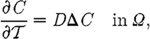
While the details between morphogen-mediated patterning mechanisms are different, they all rely on three basic processes: (i) production/secretion from a source, (ii) transport by diffusion, convection or transcytosis, and (iii) reaction with receptors, other regulators and/or DNA (Lander et al. 2002; Reeves et al. 2006; Umulis et al. 2006, 2008; Coppey et al. 2007, 2008; Gregor et al. 2007; Ben-Zvi et al. 2008). Consider the simple reaction–diffusion equation that describes morphogen transport by diffusion with chemical reactions

1.1

Here, u is the chemical morphogen [M/L³] (quantities in [ ] denote units: M, quantity; L, length; T, time); D is the diffusion coefficient [L²/T]; Δ≡▽² is the Laplace operator [1/L²]; τ is a characteristic time scale [T] for the chemical reactions; and R is the vector of chemical reactions [M/L³] that regulate the morphogen. Even in a very simple description of a morphogen-patterning process as shown by equation (1.1), it is clear that the solution will depend on the balance of time scales associated with diffusion and chemical reactions, specific boundary conditions and geometry of Ω.

To identify conditions of morphogen scale invariance, suppose that the solution of equation (1.1) for the dynamic morphogen distribution can be represented as a product of independent functions of the form , as commonly occurs in the solution of linear systems. Many morphogen systems can be represented as the product of these functions, even if one cannot find an exact solution for each function. Here, u is the concentration; x is the position; t is the time; p is the vector of parameters; L is a scalar characteristic length for the system; and Λ_n, ϕ_n and ψ_n represent the amplitude, shape and dynamics, respectively, for each component of the series solution. Specific examples of Λ_n, ϕ_n and ψ_n are given later herein. Here, one can determine the sensitivity of each of Λ_n, ϕ_n and ψ_n to perturbations of p and L to gain insight into the dominant parameters that affect each characteristic of morphogen patterning. With the product solution, it is clear that to ensure dynamic scale invariance, three conditions must be met: (i) each amplitude (Λ_n) is independent of L, (ii) each shape function (ϕ_n) stretches appropriately in the x-direction with respect to changes in the length L, and (iii) the time-dependent functions (ψ_n) are independent of L.

Herein, the specific choices for concentration, time and length scales were varied to analyse three stages of dynamic morphogen-mediated patterning: (i) boundary-layer dynamics near the source for very early times, (ii) intermediate receptor–ligand dynamics of binding and release, and (iii) long-time dynamics of morphogen patterning at the tissue scale. Each regime is nonlinear; however, for the boundary-layer and long-time regimes, the system is approximately linear under appropriate assumptions, which allows for more detailed analysis and the identification of conditions for dynamic scale invariance. To explore the validity of the approximate analytical solution, the results were compared with finite-element numerical solutions of the full system of partial differential equations.

By using the product solution of the linear approximations for a basic model of morphogen production, transport and reaction, a number of experimentally testable conditions for equilibrium and dynamic scale invariance were identified for a class of morphogen-mediated patterning mechanisms. The main result is summarized in box 1 and many additional details and explanations are provided throughout the text to account for numerous additional insights into the dynamics of morphogen-mediated pattern formation. The conservation of the total number of binding sites, total input flux of morphogen molecules and relatively high receptor density can lead to automatic scale invariance of the morphogen at steady state and during the transient approach to steady state.

Box 1. Summary of main result for dynamic morphogen scale invariance.

A remarkable feature of organism development is the ability of patterning mechanisms to reliably produce consistent proportions between individuals that vary greatly in size. The preservation of proportion or ‘scale invariance’ is manifest in numerous different biological contexts and has been directly demonstrated in one of the earliest patterning events in Drosophila: A/P patterning by the morphogen bicoid (see main text for references). Most morphogens (including bicoid) develop a spatially non-uniform distribution in the course of a few hours; however, there is increasing evidence that many morphogen distributions never reach steady state and cells continuously respond to the dynamic evolution of the morphogen. Dynamic scale invariance means that the regulation of gene expression occurs at the same relative position and at the same time between tissues/organisms that differ in size. For example, dynamic scale invariance would ensure that the boundary of gene expression for the Bcd target hunchback would occur at 50 per cent embryo length (L) after the same duration of development regardless of the individual organism sizes.

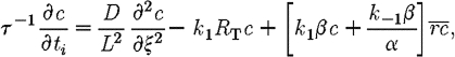
Preservation of proportion is not a property of reaction–diffusion systems in general, but the analysis herein suggests that it may be a property of numerous morphogen-patterning mechanisms that involve the diffusion (with rate D) of a morphogen (C) that binds to sites (R) with rates k₁ and k₋₁ to form , which undergoes endocytosis/decay with rate k_e as shown in the following equations:

and

Here is time; x is position; j is the input flux at the source; and R_T is the total binding site density. Substituting scaled position ξ=x/L into equation (B 1), and solving for the long-time behaviour of the system, leads to ((2.33) in text)

For convenience, conditions for steady-state scale invariance are identified first and the results are extended to analysis of the dynamic problem. At steady state, the solution of equation (B 5) is approximately exponential (for the range exhibited by most morphogens), which gives

and

The steady-state shape of the distribution will be scale invariant if λ is independent of the length L. Since D, k_e and K_m are constants, this requires R_T∝L⁻², which occurs automatically in patterning contexts that: (i) conserve the total number of binding sites, receptors or nuclei (constant total number N_T), and (ii) have similar geometries so that R_T=σN_T/L² where σ is a geometric proportionality constant. The amplitude C₀ in equation (B 6) additionally requires that: (iii) the total morphogen production at the boundary (molecules/time) is constant ((3.8) in text).

Substituting R_T=σN_T/L² into equation (B 5) gives

By inspection of equation (B 8), dynamic morphogen scale invariance additionally requires: (iv) that σN_T/L²≫K_m in which case f(L)→1. This means that the binding site density R_T is greater than the K_m value (approximate K_m values range from 1 to 1000 nM). How does binding lead to dynamic scale invariance? Binding of morphogens to immobile sites R_T dynamically slows diffusion. Lowering the binding site density by increasing the length L increases the effective diffusion by an amount that exactly offsets the longer time it takes for diffusion in a larger domain. The boost in effective diffusion leads to a system that is scale invariant dynamically and at steady state.

2. Results

While the specific biological mechanisms of morphogen-mediated patterning are very different in different contexts (figure 1), the underlying physical processes that establish a non-uniform morphogen distribution are quite similar. Consider three different morphogen processes that occur in Drosophila: (i) diffusion and nuclear import/export of a transcription factor in a syncytium as occurs for Bcd and dpERK signalling (figure 1a; Gregor et al. 2005, 2007; Coppey et al. 2008), (ii) diffusion in a thin fluid layer over a field of cells with receptor binding and endocytosis as occurs as a component of BMP patterning of the dorsal surface (figure 1b; Mizutani et al. 2005; Wang & Ferguson 2005; Umulis et al. 2006), and (iii) diffusion and receptor binding around columnar epithelial cells as occurs in the wing imaginal disc (figure 1c; Reeves et al. 2006). In each of the examples, the mechanism of morphogen removal occurs in a region that can be approximated as a two-dimensional surface: (i) binding to DNA in nuclei located at the periphery of a syncytial embryo, (ii) receptor binding and endocytosis on a cellular membrane, and (iii) binding to receptors located along the basolateral region of columnar cells. Under appropriate geometric simplifications and assumptions (details given elsewhere), each morphogen process can be approximated as a thin sheet that extends in the x-direction. Assume that the surface reactions involve only binding to a receptor and decay of the receptor–ligand complex, and to simplify the analysis, suppose that the total amount of receptors on the surface is constant in time. Here, the term receptor is used loosely to more generally mean binding sites that can represent regions of specific and non-specific binding of a transcription factor to DNA, the binding to and subsequent transport through nuclear pore complexes, or binding to receptors located on a cellular membrane. Let L_x, L_y and L_z be the lengths in the x-, y- and z- directions, respectively, and let C be the concentration of a morphogen in the fluid and R_S the concentration of receptor on the surface z=0. Suppose there is a fixed influx of C on the boundary x=0, and zero flux on the remaining faces except z=0, then the governing equations can be written as follows:

2.1

2.2

2.3

2.4

and

2.5

Figure 1.

Example geometries of morphogen-patterning pathways. (a) Diffusion and nuclear import. (b) Extracellular diffusion with receptor binding and internalization over a field of cells. (c) Diffusion through an extracellular matrix with binding along the basolateral membrane.

Here, C is the bulk concentration of the morphogen [M/L³]; R_S and are the free and bound binding sites on the surface [M/L²]; is the time; k₁ and k₋₁ are the forward and reverse binding rates of C to R with units [(M/L³.T)⁻¹] and [T⁻¹], respectively; and k_e is the decay/removal rate with units [T⁻¹]. Assuming that the initial condition of free receptors is at equilibrium and the initial levels of C are zero, then R_ST=ϕ_R/k_e for all time. As a result, the total amount of receptor is constant at every point on the surface z=0, which leads to the conservation condition (where R_ST is a constant total level of receptors).

Furthermore, if , then equations (2.2)–(2.4) can be averaged over L_z, which leads to a volumetric receptor density and R, where , and . In this scenario, the equations for receptor binding on one surface in a thin gap are completely equivalent to a system that has a uniform volumetric binding site density, such as binding sites in the extracellular matrix or import/export in nuclei. In view of the boundary conditions, the solution must be constant in the y- direction since the initial conditions are constant in the L_y-direction. This gives the simplified equations

2.6

2.7

2.8

and

2.9

To understand the solution over different length and time scales, equations (2.6)–(2.9) are non-dimensionalized by the general scalings α, β, L and τ, which non-dimensionalize the concentration c=C/α, concentration , position ξ=x/L and time (i=1, 2, 3 for the early-, intermediate- and long-time behaviour, respectively). Equations (2.6)–(2.9) reduce to

2.10

2.11

and

2.12

2.1. Time-scale analysis

The dynamics of morphogen reaction and transport in equations (2.10)–(2.12) occur on multiple time scales. For instance, one would expect that the time scale for receptor equilibration is much faster than that for transport by diffusion and other processes. To gain insight into the balance of the processes that govern morphogen dynamics on different time scales, one must make appropriate choices for τ, α, β and L in an effort to find a solution that captures the fast, intermediate and slow dynamics. The system has many possible lengths, concentration and time scales, and different combinations can be applied to study the behaviour in different regimes. It is not clear a priori what the appropriate choices for τ, α and β are for the different regimes, so that many possible parameter combinations and a brief description of the parameter group are listed in table 1.

Table 1.

Time and concentration scales. ((bl) denotes boundary layer. Magnitude is a qualitative estimate of the relative rate, concentration or length, and cross-comparisons should only be made between those in the same regime: either boundary layer (bl) or for longer times, i.e. the τ_Rδ time scale is slow when compared with other boundary-layer processes, whereas τ_R is relatively fast when compared with other processes that regulate the long-time behaviour. Note that the scalings l_m, K_m, R_T, τ_B, τ_U and τ_E are the same for both the boundary-layer and longer time dynamics.)

parameter	(symbol) description	magnitude	units	reference
Lx	(Lx) system length	variable	[L]	—
	(lm) minimum diffusion length scale	?	[L]	—
C0	(C0) scaling concentration of C	small	[M/L3]	Shimmi & O'Connor (2003)
(k−1+ke)/k1	(Km) concentration of half-maximal occupancy	?	[M/L3]	Shimmi & O'Connor (2003)
RT	(RT) total binding site concentration	variable	[M/L3]	estimate; Lauffenburger & Linderman (1993)
RTC0/(Km+C0)	equilibrium concentration	variable	[M/L3]	estimate
	(τD) diffusion time for Lx	slow	[T]	Gregor et al. (2005); Lauffenburger & Linderman (1993)
(k1C0)−1	(τC) production of by binding	fast	[T]	estimate
(k1RT)−1	(τB) removal of C by binding	fast	[T]	estimate
(k−1)−1	(τU) release of C from the binding site	fast	[T]	Umulis et al. (2006)
(ke)−1	(τE) endocytosis rate of	slow	[T]	Mizutani et al. (2005)
(k1C0+k−1+ke)−1	(τR) measure of receptor equilibration	fast	[T]	estimate
C0Lx/j	(τj) input flux time scale	slow	[T]	estimate
boundary-layer groups
lx	(lx) boundary-layer length	small	[L]	—
Cδ	(Cδ) scaling concentration of C (bl)	small	[M/L3]	Shimmi & O'Connor (2003)
RTCδ/(Km+Cδ)	equilibrium concentration (bl)	?	[M/L3]	estimate
	(τDδ) diffusion time for lx (bl)	fast	[T]	estimate
(k1Cδ)−1	(τCδ) production of by binding (bl)	slow	[T]	estimate
(k1Cδ+k−1+ke)−1	(τRδ) measure of receptor equilibration (bl)	slow	[T]	estimate
Cδlx/j	(τjδ) input flux time scale (bl)	fast	[T]	estimate

The concentration scale K_m is equivalent to the Michaelis–Menten constant and is defined by K_m=(k₋₁+k_e)/k₁. The subscript δ denotes that the time scale is defined for the boundary layer δ.

If the concentration of ligand and receptor is initially zero everywhere, the early dynamics should be governed by processes a short distance (l_x) from the source at the boundary. Specifically, the early dynamics will be governed by the input flux (τ_jδ), short-range diffusion (τ_Dδ) and receptor binding (τ_B). A short time after that, other processes, such as receptor equilibration (τ_R), endocytosis (τ_E) and long-range diffusion (τ_D), contribute to the dynamics over the full length L_x. In the following sections, a number of different time-scale hierarchies are selected to analyse the boundary-layer, intermediate- and long-time regimes, which are applicable to numerous biological pathways.

2.2. Part I: boundary-layer dynamics

It is difficult to select a characteristic length for the boundary layer (l_x) a priori, so it is assumed to be sufficiently small so that the boundary-layer dynamics are faster than all the other processes. Choosing L=l_x for the length scale, τ_jδ=C_δl_x/j, so that for the time scale, α=C_δ and β=R_TC_δ/(K_m+C_δ) for the concentration scales and substituting them into equations (2.10)–(2.12) leads to the following equations:

2.13

2.14

and

2.15

The very early dynamics of ligand (c) and bound receptor can be easily understood by the analysis of the relative time scales in equations (2.13)–(2.15). First, assume that in this scale, . All the kinetic terms in equations (2.13) and (2.14) disappear and the very early dynamics are determined solely by the flux at the boundary (2.15) and diffusion away from the source (2.13). If the flux time scale is much shorter than the diffusion time scale , the ligand accumulates at the source without diffusing away. If the diffusion time scale in the boundary is shorter than the input flux time scale , then the ligand immediately diffuses away from the source, the flux term is essentially zero and nothing appears to happen. When the flux and diffusion time scales are of the same order of magnitude (τ_Dδ≈τ_jδ), the boundary-layer equations give rise to a diffusion equation with a constant source at x=0 and diffusion coefficient τ_jδ/τ_Dδ. These three scenarios represent the very short-time behaviour at the source before any appreciable receptor binding.

Shortly after production at the boundary begins, receptor binding (τ_B) occurs close to the source. Early during patterning, there will be an excess of binding sites relative to ligand levels (i.e. ), which means that . Suppose that , defining ϵ_δ=τ_B/τ_Rδ and noting that τ_Rδ<τ_Cδ,τ_U (by definition), equations (2.13)–(2.15) lead to the following equations, with a source at ξ_δ=0:

2.16

2.17

and

2.18

In the t₁ time scale, this simplifies to a linear reaction–diffusion equation on a semi-infinite interval in the limits (lim l_x→0, lim ϵ_δ→0)

2.19

and

2.20

Here, the diffusion coefficient is , the decay term is and the flux is . Solving equation (2.19) with the boundary condition (2.20) gives

2.21

Solutions of the very short-time dynamics given by equation (2.21) are plotted along with the finite-element solution of equations (2.10)–(2.12) in figure 2a.

Figure 2.

(a) Solutions from the finite-element method (FEM) simulation of equations (2.6)–(2.9) (solid line), boundary-layer equation (2.21) (dashed line) and equation (2.39) (dotted line). (b) Plot of the L^∞ norm for the boundary-layer (solid line) and long-time (dotted line) solutions versus the FEM solution.

2.3. Part II: intermediate- and long-time dynamics

2.3.1. Intermediate dynamics

Following the short-time dynamics in the boundary layer, other processes determine the intermediate dynamics. Two important parameter groups that relate the different time scales are ϵ₁=τ_R/τ_E and ϵ₂=τ_B/τ_D. The first (ϵ₁) relates the ratio of the time scale of receptor equilibration (τ_R) to the time scale for the total loss of C by endocytosis/decay of the complex (τ_E), and ϵ₂ relates the time scale that C is absorbed by binding sites (τ_B) to the time scale for diffusion (τ_D). As will be shown later, for a reasonable morphogen profile, 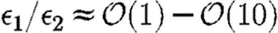and more evidence for this is given later herein. Substituting α=C₀, β=R_TC₀(K_m+C₀)⁻¹ and τ=τ_R so that , ϵ₁ into equations the following and rearranging gives the following equations for the intermediate dynamics:

2.22

2.23

2.24

2.25

and

2.26

It appears that on the intermediate time scale, equation (2.22) is governed principally by the receptor equilibration kinetics; however, it is not clear at this point whether the ratio of time scales for receptor equilibration to receptor binding (τ_R/τ_B) is large or small. If small, the receptor-binding kinetics do not play a major role in the dynamics of c, even on the intermediate time scale. As expected, for equation (2.23), the receptor-binding kinetics dominate the evolution of . Equations (2.22)–(2.24) for the intermediate time scale are nonlinear and provide limited additional information about the dynamic evolution of c. However, the intermediate scale leads naturally to the slower time scale that corresponds to the long-time and long-range morphogen patterning.

2.3.2. Long-time dynamics

After the initial boundary-layer formation and initial receptor-binding kinetics when or , the slower processes of long-range diffusion and ligand endocytosis/decay dictate the dynamics of the morphogen distribution.

Defining t₃=ϵ₂t₂ and substituting this into equations (2.22) and (2.23) rescales the equations for and c for large times,

2.27

and

2.28

Adding equations (2.27) and (2.28) gives the following equation for the total amount of morphogen (free+receptor bound):

2.29

Taking the limit ϵ₂→0 of equations (2.27)–(2.29) with the condition that ϵ₁/ϵ₂→const. leads to an algebraic equation for and the long-time behaviour for the total amount of ligand. Solving for , calculating the derivative of with respect to t₃ and substituting the solution into equation (2.29) gives

2.30

2.31

and

2.32

2.4. Solution of linear approximation for long-time dynamics

The resulting equation for the long-time behaviour of unbound c is a nonlinear PDE with no general solution. However, the equation is linear if the level of ligand C₀ is small, so that the total amount of bound ligand is far from saturation. Specifically, this requires , so that , and equation (2.31) becomes a linear non-homogeneous PDE,

2.33

2.34

2.35

and

2.36

By introducing v(ξ,t₃)=c(ξ,t₃)−c_E(ξ), where c_E(ξ) is the equilibrium solution, the above non-homogeneous PDE for c(ξ,t₃) is converted into a simpler homogeneous PDE in the displacement variable v(ξ,t₃). The equilibrium solution for equations (2.33)–(2.36) is

2.37

and

2.38

Also, the exact transient solution is

2.39

2.40

and

2.41

The solution for the linear approximation with n=100 is shown along with a finite-element solution of equations (2.6)–(2.9) for very early times in figure 2a,b and the equilibrium solution (2.37) is shown in figure 3a for . As shown in figure 2a,b, the long-time behaviour better approximates the finite-element method (FEM) solution after the first 100 s (parameters are listed in the caption to figure 3). Figure 3b shows the transient evolution of c(ξ,t₃) at ξ=0, 0.2, 0.4 for the linear approximation versus the FEM solution for long times. Figure 3a,b demonstrates that the linear approximation captures the equilibrium and dynamic behaviour of the full nonlinear system when . Note that C₀ is determined by setting ξ=0, c_E(0)=1 in equation (2.37). As expected, the linear approximation breaks down as C₀→K_m both at equilibrium (figure 3c) and dynamically (figure 3d).

Figure 3.

(a) Example equilibrium solution for the linear approximation (solid line, c_E(ξ)) and finite-element solution of the full problem (open circles, c_FEM(ξ)). (b) Comparison of dynamics in the linear approximation (solid line, C_linear) versus the FEM solution (dotted line, c_FEM) of the full system at positions ξ=0, 0.2 and 0.4. (c) Accuracy of linear approximation depends on the ratio of C₀/K_m. As C₀/K_m increases, the approximation and the FEM solution diverge both at (c) equilibrium and (d) dynamically. T₉₀ is the time it takes to reach 90% of the equilibrium value at ξ=0 (solid line), ξ=0.2 (dashed line) and ξ=0.4 (open circles). For the figures herein, the following parameter values are used: D=20 μ² s⁻¹; k₁=5×10⁻³ nM⁻¹ s⁻¹; k₋₁=1×10⁻² s⁻¹; k_e=5×10⁻⁴ s⁻¹; N_tot=10⁵ molecules; ρ=0.1; L_z=1 μm; and Φ=22 molecules min⁻¹.

3. Conditions for scale invariance

The solutions for the early- and long-time dynamics of equations (2.6)–(2.9) provide a framework to investigate plausible mechanisms of biological scale invariance. To make the analysis more straightforward, conditions for scale invariance of the equilibrium solution are identified first, followed by a brief analysis of the boundary layer and a more extensive analysis of the long-time behaviour of the system. Since the time scale of many morphogen-mediated pathways is of the order of tens to hundreds of minutes, the long-time and equilibrium behaviours are most relevant for real biological morphogen pathways.

3.1. Conditions for scale invariance of the equilibrium solution

The equilibrium solution (2.37) can be represented as a product of an amplitude and shape function, c_E(ξ,p,L_x)=Λ(p,L_x).ϕ(ξ,p,L_x).

Equation (2.37) can be rewritten as

3.1

Now substituting the parameters and into 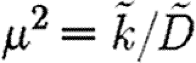gives

3.2

Earlier, it was speculated that the ratio for a reasonable morphogen profile. Since in this context, it follows that θ⁻¹≈1 and the decay length of the morphogen distribution at equilibrium is determined solely by μ≈(ϵ₁/ϵ₂)^1/2. If , the equilibrium solution decays rapidly from the source, and the range of the morphogen would be too short to effectively pattern a field of cells in a concentration-dependent manner. If , the shape of the morphogen distribution will be essentially flat over the field of cells and thus neighbouring cells would adopt identical fates. For , it constrains the maximum of the ratio of time scales to . What does mean? Substituting the parameters back into μ² gives

3.3

Equation (3.3) is a ratio of a measure of the diffusion time against a grouping of binding, equilibration and removal kinetic time scales. In essence, means that the kinetic and diffusion time scales are of the same order of magnitude and since the distribution of morphogen is determined by a balance between the time scales, it leads to an overall length scale of morphogen appropriate for having sufficient range and sufficient slope for patterning.

The shape ϕ will be scale invariant if and only if μ is independent of L_x. It is readily apparent that μ is independent of the system length (L_x) if , since D, k_e and K_m are constant parameters. Substituting R_T=N_T/L_xL_yL_z into equation (3.3) makes the requirements for scale invariance more transparent in the following equation:

3.4

Given equation (3.4), and since k_e, D and K_m are constant, μ² will be independent of L_x and the equilibrium shape function (ϕ) will be scale invariant if is also constant. A number of scenarios can hypothetically ensure a constant ratio and the two most biologically tenable options are the following: (i) the total number of binding sites (N_T) scales in proportion to with fixed L_y, L_z, or (ii) N_T remains constant and the product of L_xL_yL_z is proportional to . While the first possibility cannot be ruled out since there may be mechanisms that carefully regulate N_T in proportion to , the indirect evidence (detailed in §1) suggests that the second possibility of constant N_T and appropriate scaling of L_xL_yL_z may contribute to scale invariance for a number of morphogen-patterning mechanisms.

These observations suggest that (i) N_T may be constant between organisms within and between species at the same developmental stage (Teleman & Cohen 2000; Gregor et al. 2005), (ii) different-sized organisms have similar proportions so that L_y=ρL_x, where ρ is the proportionality constant (Gregor et al. 2005), and (iii) the total input flux may be constant (specifically for wing disc patterning by Dpp; Teleman & Cohen 2000). Lastly, it is assumed that the height of the gap for diffusion (L_z) is constant, which is expected since the distance between cells, the thickness of the cortical layer or the thickness of the perivitelline space are intrinsic to the cell biology that develops those regions and not the scale of the system. With these conditions, μ² can be rewritten as

3.5

where

3.6

In other words, the shape function ϕ is independent of L_x under conditions of (i) constant total number of binding sites, (ii) constant gap height L_z, and (iii) uniform dilations in tissue size.

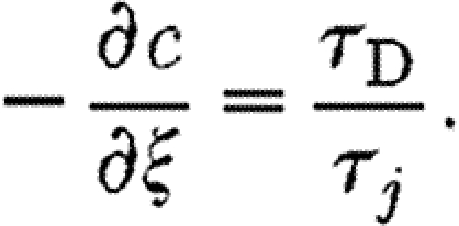
If μ is independent of L_x, the amplitude Λ will be invariant if J scales appropriately for changes in the system length. However, J=τ_D/τ_j=jL_x/(DC₀) and amplitude invariance can only be achieved if .

One plausible mechanism that ensures the proper scaling of j occurs when the total input number flux Φ is constant instead of the flux density j. On a two-dimensional sheet as analysed here, this leads to

3.7

that is,

3.8

Substituting equation (3.8) into J and noting that L_y/L_x=ρ, a constant, it follows that J=Φ(ρL_zDC₀)⁻¹ and so Λ is independent of L_x. As expected, when the conditions for equilibrium scale invariance are met, the distribution of morphogen shifts in proportion to the length of the system, as shown in figure 4a in x-coordinates. When remapped onto ξ∈[0,1], the profiles are superimposed over each other as shown in figure 4b.

Figure 4.

(a) Equilibrium solution for the linear approximation versus position for systems with characteristic lengths (L_x) of 10 μm (solid line), 100 μm (open circles) and 1000 μm (dotted line). (b) Same as in (a) rescaled to the interval [0, 1]. (c) Plot of the exponential term that depends on the system length versus R_T/K_m (left axis). Time to reach 90% of the equilibrium concentration at ξ=0 versus R_T/K_m (right axis) for the finite-element model. (d) Dynamic scale invariance by conservation of binding sites is ensured if .

3.2. Analysis of boundary-layer dynamics

For the very early dynamics, the characteristic time scale is related to the flux of molecules into the system at the boundary (τ_jδ=C_δl_x/j). The time scale inherently depends on the choice of the characteristic length used to study the boundary-layer dynamics (l_x). To determine whether the very early dynamics are scale invariant, the solution is remapped to actual time () and scaled position ξ∈[0,1]. Equation (2.21) then becomes

3.9

In equation (3.9), it is clear that the very early dynamics in the boundary layer are not scale invariant since the time () is scaled by the overall length L_x.

3.3. Conditions for long-time dynamic scale invariance

In addition to the steady-state morphogen distribution, the morphogen dynamics are also important in a number of biological contexts. Equations (2.39)–(2.41) were further analysed to determine (i) the rate of approach to the equilibrium solution, and (ii) whether it is possible to achieve scale invariance dynamically, i.e. the morphogen distribution in different-sized domains is proportional for all times during the transient evolution of the distribution.

Since c(ξ,t₃)=c_E(ξ)+v(ξ,t₃) and c_E(ξ) is scale invariant by the conditions outlined in §3.1, it follows that will be scale invariant if each of the Λ_n, ϕ_n and ψ_n is independent of L_x.

Here, the solution is represented by a sum of terms as shown in the following by rearranging equations (2.39)–(2.41):

3.10

3.11

3.12

3.13

3.14

and

3.15

The conditions for scale invariance identified in §3.1 make the analysis of dynamic scale invariance straightforward. First, since , there is a direct relationship between actual time () and scaled time , which means that if t₃ is independent of L_x, then the actual time () is also independent of L_x.

It is immediately apparent that the shape functions (ϕ_n) are scale invariant; however, it is not clear whether the Λ_n and ψ_n are independent of L_x. Recalling that θ≈1 and that J and μ are independent of L_x (§3.1), and substituting and into equations (3.11) and (3.12) for Λ_n gives

3.16

which is automatically independent of L_x.

Next, substituting and into equation (3.14) (ψ_n) gives

3.17

and recalling

3.18

the conditions for dynamic scale invariance are more transparent. Whether or not the morphogen evolution is scale invariant depends on the ratio of R_T to K_m. Substituting R_T/K_m into equation (3.17) gives

3.19

If receptor density relative to the K_m value is small so that , then equation (3.19) becomes

3.20

and the time it takes to reach equilibrium increases in proportion to the length of the system squared. In the other limit

3.21

and the dynamics of the morphogen distribution are completely independent of the length of the system.

Figure 4c (left axis) shows how the value of the leading term associated with each exponential depends on the ratio of R_T/K_m, which provides an indication of the time it takes to reach equilibrium. Figure 4c (right axis) shows the time it takes for the FEM solution to reach 90 per cent of the equilibrium values for a given set of parameters. As R_T/K_m increases, the exponential term becomes more negative, which means the solution approaches equilibrium more rapidly until levelling off at a constant value, which is consistent with the behaviour of the FEM solution of the full model. However, since , for fixed , this places limits on the maximum size for which dynamic scale invariance occurs automatically. Specifically, dynamic scale invariance requires that (figure 4d).

What does this mean for real biological systems? The ratio τ_R/τ_B in equation (3.17) represents the relationship between time scales of binding site equilibration to the time scale of ligand binding and removal from the freely diffusing pool. While τ_R/τ_B emerged as an important relationship between time scales, it can also be interpreted as a ratio of the concentration scales R_T/K_m. In this context, the ratio of R_T to K_m relates the total binding site density to the concentration of ligand necessary to achieve 50 per cent binding site occupancy. A small R_T/K_m suggests either a very low concentration of receptors or very weak binding (either a slow on-rate or a fast off-rate). With relatively few binding sites or weak binding, diffusion is largely unhindered and changing the binding site density has little effect on the dynamics of transport, which leads to an increase in the time it takes to approach steady state. On the other hand, a large R_T/K_m suggests either a high receptor concentration or tight binding. The large number of binding sites transiently slows the diffusion process and decreasing the density of binding sites leads to a faster effective diffusion. For a range of parameter values, if the binding site density decreases as L_x increases, the effective diffusion constant increases in proportion to . The boost in effective diffusion leads to a system that is scale invariant both dynamically and at equilibrium.

4. Discussion

In this paper, multiple time scales are used to better understand the dynamics and identify conditions for scale invariance of morphogen-mediated patterning. The principal conditions that lead to scale invariance of a morphogen distribution are

• — conservation of the total number of binding sites for the morphogen;

• — conservation of the total number of morphogen molecules secreted in a given length of time at the boundary;

• — for scale invariance of morphogen gradient interpretation, cells (or nuclei) must respond to the total occupancy of receptors and not to the surface density of occupied receptors (appendix A); and

• — for dynamic scale invariance, there needs to be an excess of binding sites on the surface to slow the effective diffusion.

The properties for dynamic scale invariance are based on evidence from a number of different pathways and the analysis suggests that the simple mechanism of binding and release may contribute to scale invariance. While supported by observations, a number of theoretical and experimental studies will further delineate mechanisms of scale invariance in different contexts. The model presented here depends on a number of assumptions, and future work should be extended to include the following: (i) non-uniform binding site density as occurs in wing imaginal disc patterning by Dpp (Lecuit & Cohen 1998; Teleman & Cohen 2000; Serpe et al. 2008), (ii) binding site density that changes in time (Umulis et al. 2006; Gregor et al. 2007; Coppey et al. 2008; Serpe et al. 2008), (iii) feedback from receptor signalling (Fujise et al. 2003; Wang & Ferguson 2005; Umulis et al. 2006), (iv) nonlinear extracellular regulation as occurs in dorsoventral patterning of Drosophila and Xenopus embryos (Mizutani et al. 2005; Shimmi et al. 2005; O'Connor et al. 2006; Umulis et al. 2006, 2008; Ben-Zvi et al. 2008), (v) more detailed analysis of nuclear import/export kinetics (Coppey et al. 2007, 2008; Gregor et al. 2007), (vi) transcytosis through columnar epithelial cells (Kruse et al. 2004; Bollenbach et al. 2005; Kicheva et al. 2007), and (vii) more realistic geometries of the underlying tissues. The analysis presented herein serves as a starting point for future analysis, but it also serves as the common theme that links the diverse morphogen pathways.

The conditions for scale invariance are general enough that they can be tested in a number of different contexts. For instance, one could measure the distribution of pMad signalling and extracellular Dpp–green fluorescent protein (Kicheva et al. 2007) in the posterior compartment of wing discs that ectopically express cyclin-dependent kinases to increase or decrease the number of cells. Furthermore, additional experiments such as changing the binding site density (receptors, Cv-2, etc.) during D/V embryonic patterning by BMPs, disrupting the nuclear density during A/P patterning by Bcd, measuring the time it takes for A/P pattern formation by Bcd in different-sized embryos or altering the geometry of a developing tissue would all provide additional insight into the mechanisms of biological scale invariance.

In summary, morphogens mediated by diffusion, binding and endocytosis/degradation can yield scale invariance automatically if the number of binding sites is conserved for changes in system size. As mentioned in Gregor et al. (2007), this may lead to scaling of bicoid. For systems with excess binding sites, scale invariance may occur dynamically as well as at equilibrium.

Appendix A

A.1. Ligand decay

In addition to endocytosis or decay of morphogen from binding sites, one could envision a related but mechanistically different process where the morphogen has an intrinsic lifetime that may or may not be affected by binding. For instance, if the morphogen is a transcription factor that is diffusing over a field of nuclei, the bound and unbound states do not undergo endocytosis as in receptor ligand systems and one would expect similar decay times for the bound and unbound morphogens. In essence, this adds a decay term to the equation for unbound ligand in equation (2.1). Using analogous analysis to that developed herein, the extra kinetic step introduces another ratio of time scales ϵ₃=k_c/(k₁(K_m+C₀)). This gives

A1

If the decay rates in the bound and unbound states are equal, then ϵ₁=ϵ₃. Scale invariance at equilibrium is assured if , in which case the majority of morphogens is in the bound state and the contribution of unbound decay is negligible.

A.2. Scale invariance of receptor–ligand systems

The above analysis demonstrates how scale invariance can be achieved if the binding site density scales as L²; however, it is more important that the interpretation of the signal scales properly as well. In the case of nuclei and transcription factor systems such as A/P patterning in Drosophila, the local concentration at discrete sites is constant for changes in system size so that the scale invariance at the level of occupied binding sites is automatic. For ligand–receptor systems, the extracellular gradient scales by reducing the concentration of binding sites. Since receptor concentrations decrease for increases in size, the surface density of receptor-bound ligand also decreases. Thus, the concentration of ligand-bound receptors is not scale invariant and cells must interpret the signal by another mechanism. One possibility for morphogen interpretation is to integrate the signal over the entire surface of each cell into a downstream response. In essence, cells count the total number of ligand-occupied receptors to initiate a downstream response as has been shown for activin signalling (Dyson & Gurdon 1998). Suppose cells are spaced in a square lattice with dimensions l_x=aL_x and l_y=bL_y. Mathematically, for a square surface arranged in a regular array, the total signal is represented by

A2

Here, is the total number of occupied receptors on the surface of the cell specified by position n, m, at time t₃. The constants a and b correspond to the fractional length of a cell in scaled coordinates. To show that the integral of receptors on the surface scales, apply the first mean-value theorem for integrals, which states that there exists some c∈[a,b] such that the following equality is true:

A3

This leads to the following expression for the number of ligand-occupied receptors per cell:

A4

Then, the mean-value theorem for integration of a single cell gives

A5

and

A6

Since c_E(ξ) is independent of L_x, it follows that ξ^* is independent of L_x only if v(ξ,t₃) is independent of L_x by the conditions shown herein.

References

- Ben-Zvi D., Shilo B.-N., Fainsod A., Barkai N. 2008. Scaling of the BMP activation gradient in Xenopus embryos. Nature. 453, 1205–1211. ( 10.1038/nature07059) [DOI] [PubMed] [Google Scholar]
- Bergmann S., Sandler O., Sberro H., Shnider S., Schejter E., Shilo B.-Z., Barkai N. 2007. Pre-steady-state decoding of the bicoid morphogen gradient. PLoS Biol. 5, e46 ( 10.1371/journal.pbio.0050046) [DOI] [PMC free article] [PubMed] [Google Scholar]
- Bollenbach T., Kruse K., Pantazis P., González-Gaitán M., Jülicher F. 2005. Robust formation of morphogen gradients. Phys. Rev. Lett. 94, 018 103 ( 10.1103/PhysRevLett.94.018103) [DOI] [PubMed] [Google Scholar]
- Coppey M., Berezhkovskii A.M., Kim Y., Boettiger A.N., Shvartsman S.Y. 2007. Modeling the bicoid gradient: diffusion and reversible nuclear trapping of a stable protein. Dev. Biol. 312, 623–630. ( 10.1016/j.ydbio.2007.09.058) [DOI] [PMC free article] [PubMed] [Google Scholar]
- Coppey M., Boettiger A., Berezhkovskii A., Shvartsman S. 2008. Nuclear trapping shapes the terminal gradient in the Drosophila embryo. Curr. Biol. 18, 915–919. ( 10.1016/j.cub.2008.05.034) [DOI] [PMC free article] [PubMed] [Google Scholar]
- Dyson S., Gurdon J. 1998. The interpretation of position in a morphogen gradient as revealed by occupancy of activin receptors. Cell. 93, 557–568. ( 10.1016/S0092-8674(00)81185-X) [DOI] [PubMed] [Google Scholar]
- Fujise M., Takeo S., Kamimura K., Matsuo T., Aigaki T., Izumi S., Nakato H. 2003. Dally regulates Dpp morphogen gradient formation in the Drosophila wing. Development. 130, 1515–1522. ( 10.1242/dev.00379) [DOI] [PubMed] [Google Scholar]
- Gregor T., Bialek W., de Ruyter van Steveninck R.R., Tank D.W., Wieschaus E.F. 2005. Diffusion and scaling during early embryonic pattern formation. Proc. Natl Acad. Sci. USA. 102, 18 403–18 407. ( 10.1073/pnas.0509483102) [DOI] [PMC free article] [PubMed] [Google Scholar]
- Gregor T., Wieschaus E., McGregor A., Bialek W., Tank D. 2007. Stability and nuclear dynamics of the bicoid morphogen gradient. Cell. 130, 141–152. ( 10.1016/j.cell.2007.05.026) [DOI] [PMC free article] [PubMed] [Google Scholar]
- Kicheva A., Pantazis P., Bollenbach T., Kalaidzidis Y., Bittig T., Jülicher F., González-Gaitán M. 2007. Kinetics of morphogen gradient formation. Science. 315, 521–525. ( 10.1126/science.1135774) [DOI] [PubMed] [Google Scholar]
- Kruse K., Pantazis P., Bollenbach T., Jülicher F., González-Gaitán M. 2004. Dpp gradient formation by dynamin-dependent endocytosis: receptor trafficking and the diffusion model. Development. 131, 4843–4856. ( 10.1242/dev.01335) [DOI] [PubMed] [Google Scholar]
- Lander A., Nie Q., Wan F. 2002. Do morphogen gradients arise by diffusion?. Dev. Cell. 2, 785–796. ( 10.1016/S1534-5807(02)00179-X) [DOI] [PubMed] [Google Scholar]
- Lauffenburger D., Linderman J. 1993. Receptors: models for binding, trafficking, and signaling. New York, NY:Oxford University Press [Google Scholar]
- Lecuit T., Cohen S. 1998. Dpp receptor levels contribute to shaping the Dpp morphogen gradient in the Drosophila wing imaginal disc. Development. 125, 4901–4907. [DOI] [PubMed] [Google Scholar]
- Mizutani C., Nie Q., Wan F., Zhang Y., Vilmos P., Sousa-Neves R., Bier E., Marsh J., Lander A. 2005. Formation of the BMP activity gradient in the embryo. Dev. Cell. 8, 915–924. ( 10.1016/j.devcel.2005.04.009) [DOI] [PMC free article] [PubMed] [Google Scholar]
- O'Connor M.B., Umulis D., Othmer H.G., Blair S.S. 2006. Shaping BMP morphogen gradients in the Drosophila embryo and pupal wing. Development. 133, 183–193. ( 10.1242/dev.02214) [DOI] [PMC free article] [PubMed] [Google Scholar]
- Reeves G., Muratov C., Schüpbach T., Shvartsman S. 2006. Quantitative models of developmental pattern formation. Dev. Cell. 11, 289–300. ( 10.1016/j.devcel.2006.08.006) [DOI] [PubMed] [Google Scholar]
- Serpe M., Umulis D., Ralston A., Chen J., Olson D., Avanesov A., Othmer H., O'Connor M., Blair S. 2008. The BMP-binding protein crossveinless 2 is a short-range, concentration-dependent, biphasic modulator of BMP signaling in Drosophila. Dev. Cell. 14, 940–953. ( 10.1016/j.devcel.2008.03.023) [DOI] [PMC free article] [PubMed] [Google Scholar]
- Shimmi O., O'Connor M.B. 2003. Physical properties of Tld, Sog, Tsg and Dpp protein interactions are predicted to help create a sharp boundary in Bmp signals during dorsoventral patterning of the Drosophila embryo. Development. 130, 4673–4682. ( 10.1242/dev.00684) [DOI] [PubMed] [Google Scholar]
- Shimmi O., Umulis D., Othmer H., O'Connor M. 2005. Facilitated transport of a Dpp/Scw heterodimer by Sog/Tsg leads to robust patterning of the blastoderm embryo. Cell. 120, 873–886. ( 10.1016/j.cell.2005.02.009) [DOI] [PMC free article] [PubMed] [Google Scholar]
- Teleman A., Cohen S. 2000. Dpp gradient formation in the Drosophila wing imaginal disc. Cell. 103, 971–980. ( 10.1016/S0092-8674(00)00199-9) [DOI] [PubMed] [Google Scholar]
- Umulis D.M., Serpe M., O'Connor M.B., Othmer H.G. 2006. Robust, bistable patterning of the dorsal surface of the Drosophila embryo. Proc. Natl Acad. Sci. USA. 103, 11 613–11 618. ( 10.1073/pnas.0510398103) [DOI] [PMC free article] [PubMed] [Google Scholar]
- Umulis D., O'Connor M.B., Othmer H.G. 2008. Robustness of embryonic spatial patterning in Drosophila melanogaster. Curr. Top. Dev. Biol. 81, 65–111. ( 10.1016/S0070-2153(07)81002-7) [DOI] [PMC free article] [PubMed] [Google Scholar]
- Wang Y.-C., Ferguson E.L. 2005. Spatial bistability of Dpp–receptor interactions during Drosophila dorsal–ventral patterning. Nature. 434, 229–234. ( 10.1038/nature03318) [DOI] [PubMed] [Google Scholar]
- Wolpert L. 1969. Positional information and the spatial pattern of cellular differentiation. J. Theor. Biol. 25, 1–47. ( 10.1016/S0022-5193(69)80016-0) [DOI] [PubMed] [Google Scholar]