Measuring Transcription Factor–Binding Site Turnover: A Maximum Likelihood Approach Using Phylogenies

Abstract

A major mode of gene expression evolution is based on changes in cis-regulatory elements (CREs) whose function critically depends on the presence of transcription factor–binding sites (TFBS). Because CREs experience extensive TFBS turnover even with conserved function, alignment-based studies of CRE sequence evolution are limited to very closely related species. Here, we propose an alternative approach based on a stochastic model of TFBS turnover. We implemented a maximum likelihood model that permits variable turnover rates in different parts of the species tree. This model can be used to detect changes in turnover rate as a proxy for differences in the selective pressures acting on TFBS in different clades. We applied this method to five TFBS in the fungi methionine biosynthesis pathway and three TFBS in the HoxA clusters of vertebrates. We find that the estimated turnover rate is generally high, with half-life ranging between ∼5 and 150 My and a mode around tens of millions of years. This rate is consistent with the finding that even functionally conserved enhancers can show very low sequence similarity. We also detect statistically significant differences in the equilibrium densities of estrogen- and progesterone-response elements in the HoxA clusters between mammal and nonmammal vertebrates. Even more extreme clade-specific differences were found in the fungal data. We conclude that stochastic models of TFBS turnover enable the detection of shifts in the selective pressures acting on CREs in different organisms.

The analysis tool, called CRETO (Cis-Regulatory Element Turn-Over) can be downloaded from http://www.bioinf.uni-leipzig.de/Software/creto/.

Introduction

The evolution of gene expression occurs through changes in transcriptional control mechanisms, including the modification of cis-regulatory elements (CREs) (Wray 2001; Gompel et al. 2005) and the evolution of novel functions in regulatory proteins such as transcription factors and cofactors (Lynch et al. 2008; Wagner and Lynch 2008). To date, most studies have focused on the evolution of CREs. Modification of CREs mostly consists of the acquisition and/or loss of transcription factor–binding sites (TFBS) (Istrail and Davidson 2005). Hence, investigating the molecular evolution of CREs may reveal the timing and the kind of evolutionary changes that affect gene regulation through changes in CREs similar to the success of methods for characterizing the tempo and mode of protein evolution. However, a major obstacle to the analysis of sequence evolution in CREs has been the low degree of sequence conservation among even functionally conserved CREs (Crocker and Erives 2008). Population genetic and molecular evolutionary approaches to CRE evolution have applied a number of strategies to circumvent these problems. For example, one strategy has been to first identify highly conserved noncoding sequences and then investigate the pattern and rate of nucleotide substitutions in these conserved noncoding sequences (Wagner et al. 2004; Prabhakar et al. 2006). Another approach has been to focus on closely related species, in which the sequence divergence is minimal, and to then apply population genetic methods (Wong and Nielsen 2004; Balhoff and Wray 2005; Haygood et al. 2007), but computational methods of examining the rate and pattern of CRE evolution of are still in their infancy.

In this paper, we pursue an alternative approach originally formulated by Wagner et al. (2007). In this approach, noncoding sequences are not compared on a nucleotide-by-nucleotide basis following standard molecular evolution methods, but instead, the density of TFBSs in a specific genomic region are compared across taxa. Binding sites can undergo constant turnover; thus, in this approach it is assumed that the functionally important measure is likely to be binding site “number” rather than their “location” or precise “identity.” This model further assumes that TFBSs in the genomic region of interest have a constant rate of origination λ and decay exponentially with a relative rate μ (supplementary fig. S1, Supplementary Material online) and is mathematically identical to the classical model of queuing theory called M/M/∞ (Medhi 2003). In our previous paper, we explicitly derived the transient conditional probabilities for changes in binding site number and proposed a stochastic model for TFBS evolution (Wagner et al. 2007). Applying this model to a small data set of the number of estrogen-response elements (EREs) in primate HoxA clusters showed that the pattern of ERE turnover is generally consistent with a stationary turnover process with an estimate of the half-life of about 27 My, corresponding to a per site decay rate of $\mathrm{\mu }\approx 1.3\times {10}^{-8}/\text{year}$ and a rate of origination of $\mathrm{\lambda }\approx 1.6\times {10}^{-7}/\text{year}.$ Thus, this method has the potential to infer the rate and pattern of TFBS evolution.

Here, we further develop this method into a maximum likelihood (ML) model to analyze TFBS density in an explicit phylogenetic context. The method is validated with simulated data and then applied to two data sets of TFBS density from very different systems, including transcription factors that regulate the yeast methionine biosynthesis pathway and nuclear receptor–binding sites in the HoxA clusters of vertebrates. We find strong statistical support for an increase in equilibrium-binding site density and a corresponding increase in half-life for estrogen- and progesterone-response elements in the mammalian HoxA clusters coincident with the origin of mammals. However, we found no difference in retinoic acid-response element numbers. Similar lineage-specific differences are also found in the proximal promoters of genes in the methionine biosynthetic pathway in a sample of yeast species. We conclude that the statistical analysis of binding site density data can identify potentially important changes in the selective constraints acting on CREs.

Materials and Methods

Yeast Data

The upstream regions for the predicted protein-coding genes across 13 yeast (Ascomycete) genomes (Saccharomyces cerevisiae, Saccharomyces paradoxus, Saccharomyces mikatae, Saccharomyces bayanus, Candida glabrata, Saccharomyces castellii, Kluyveromyces lactis, Ashbya gossypii, Kluyveromyces waltii, Candida albicans, Debaryomyces hansenii, Yarrowia lipolytica, and Schizosaccharomyces pombe) were obtained from Wapinski et al. (2007). Out of 27 methionine biosynthesis genes compiled by Gasch et al. (2004), eight (Met2, Met3, Met6, Met8, Met10, Met16, Met30, and Sah1) were identified as single-copy orthologous in all 13 species using the Fungal Orthogroups Repository (http://www.broad.mit.edu/regev/orthogroups/; Wapinski et al. (2007).

To determine the TFBS density, we used a compilation of 80 binding sites represented by International Union for Pure and Applied Chemistry consensus sequences (Gasch et al. 2004). We searched 500 bp upstream of our eight orthologous single-copy genes for each of the binding sites, counting the occurrences in both strands. In 41 of 104 cases, the noncoding upstream sequence was less than 500 bp, so the count was extrapolated linearly to this value (e.g., if eight binding sites were found in 400 bp of upstream sequence, our final count was assigned as 10). In two outlier cases, we instead assigned the binding site count from the closest relative to two species because they had upstream sequences of 1 and 37 bp. Out of 80 TFBSs, five were found to be enriched in the single-copy orthologous genes compared with the rest of the genome (bound by Bas1p, Cbf1p, Gcn4p, Met30/31p, and Rtg1/Rtg3p). Enrichment was inferred by applying Fisher's exact test to compare the times the binding site was found for all species in the single-copy orthologous genes (104 promoter regions total) and in the rest of genome (73944 promoters). To get the final binding site count for these transcription factors, we summed up all the occurrences in the eight related genes for each of the species. All these processes were automated using PERL scripts.

To obtain the chronogram (ultrametric tree with branch lengths proportional to time), we used the phylogenetic tree topology from Wapinski et al. (2007). For the tree reconstruction, Wapinski et al. used 10,000 amino acid residues that were randomly drawn with replacement from the concatenated alignment of all single-copy proteins. We estimated divergence times by penalized likelihood with a truncated Newton algorithm in r8s version 1.71 (Sanderson 2006) setting the smoothing parameter to 0.06. The optimization of the smoothing parameter was obtained following the instructions of r8s program manual (available at http://loco.biosci.arizona.edu/r8s/). The tree species phylogeny was calibrated by fixing the split of D. hansenii and C. albicans from the other yeast at 272 My (Miranda et al. 2006).

HoxA Cluster Data

The complete HoxA clusters from horn shark (Heterodontus francisci: AF224262, AF224263), bichir (Polypterus senegalus: AC126321 and AC132195, Chiu et al., 2004), coelacanth (Latimeria menadoensis: FJ497005), frog (Xenopus tropicalis: 3616499), bat (Rhinolophus ferrumequinum: DP000727), elephant (Loxodonda africana: NT161952), armadillo (Dasypus novemcinctus: NT108274), platypus (Ornithorhynchus anatinus: NT165289), dog (Canis familiaris: NT107854), galago (Otolemur garnettii: DP000935), mouse lemur (Microcebus murinus: NT165887), rabbit (Oryctolagus cuniculus: DP001063), cow (Bos taurus: NT107808), tamarin (Callithrix jacchus: NT113347), chicken (Gallus gallus: NT107524), opossum (Monodelphis domestica: NT113108, NT112848), dog (C. familiaris: NT107854, NT165635), rat (Rattus norvegicus: NT107474), mouse (Mus musculus: NT165680), macaque (Macaca mulatta: NT108362), chimpanzee (Pan troglodytes: NT107590), and human (Homo sapiens: NT086366), including those sequenced as part of the ENCODE project, were downloaded from NCBI. The sequence around the cluster was trimmed to include 5 kb of sequence upstream of the most 5′ Hox gene and 5 kb downstream of the most 3′ Hox gene.

Putative estrogen, progesterone, and retinoic acid-response elements were identified using in-house PERL scripts that identify and report the location of sequence motifs given as regular expressions. The consensus ERE sequence used in this study, GSYCMNNNWGAMS, was generated from the consensus identified in a genome-wide search for high-affinity response elements (Bourdeau et al. 2004) and two EREs experimentally determined to regulate HoxA-10 (Akbas et al. 2004). Only those patterns with four or fewer mismatches from the “perfect” ERE (GGTCANNNGTACC) were counted. The progesterone-response element consensus was based on experimentally determined high-affinity progesterone receptor–binding sites (Nelson et al. 1999) with a variable half-site and a fixed half-site (TCTTGTNNNACAAGA); one substitution in the six nucleotides of the fixed half-site was allowed and three mismatches to the perfect progesterone-response element (PRE) were allowed in the variable half-site. The reliability of this counting method was cross-validated against the Dragon ERE finder, which uses a hidden Markov model to identify EREs. (Dragon predictions matched our selection criteria ±2 to 3 sites in test comparisons between human, elephant, platypus and chicken.) For the detection of the retinoic acid-response element (RARE)–binding sites, we did an exact forward and reverse search of 18 experimentally defined DR5 RAREs (Mainguy et al. 2003) that consists of five defined nucleotides on each side separated by five arbitrary nucleotides.

The Algorithm

The algorithm takes as input the number of binding sites for an arbitrary but fixed transcription factor for each species and a phylogenetic tree of those species with branch lengths. In its simplest implementation, the algorithm estimates the decay rate, μ, and the origination rate, λ, for these binding sites by maximizing the likelihood of the observed binding site numbers on the tree. The likelihood is calculated based on the time-dependent conditional probability of having exactly n binding sites when t generations before the binding site number was n₀ (Wagner et al. 2007). To facilitate the detection of statistically significant differences in binding site dynamics, we also implemented a version where a subtree or subtrees can have different binding site turnover parameters (e.g., see fig. 1). Note that the parameter pair for a subtree is applied to a clade and the stem lineage of the clade. The algorithm consists of two nested optimization loops, one for maximizing the likelihood and one to improve the step length of the search algorithm (see supplementary fig. S2 [Supplementary Material online] for a schematic).

FIG. 1.—

Example of binding site number evolution for multiple turnover parameters: Phylogenetic tree with six species (A–F with 1–11 binding sites) and three parameter pairs. Each node is labeled with its unique label followed by the mean binding site number of the corresponding subtree and the difference of that number to that of the ancestor node. Because node 1 and node 11 have the largest differences, their subtrees are chosen by the program to have different rates (gray). Note that the rates are valid from the ancestor of the subtree on.

The tree likelihood L is calculated from the conditional likelihoods $L_i\left(n\right),$ that is, the likelihood of all evolutionary histories conditional on the assumption that at node i exactly n binding sites are present. The tree likelihood is then calculated as the weighted average of the conditional likelihoods of the root node r over all possible binding site numbers with the prior probability $\mathrm{\pi }\left(n\right).$ For the prior probability, we take the equilibrium distribution for the TFBS model, which is the Poisson distribution. We parameterize the Poisson distribution with the mean binding site number $\stackrel{-}{n}$ averaged over all species.

Because the number of all possible binding site numbers is potentially infinite, we have to restrict n to a finite interval for computational reasons, $n_{\min }\le n\le n_{\max }.$ For determining these values, we define a “bound” value (default is 10⁻⁶) and calculate the lowest and largest n so that the probability of the Poisson distribution from 0 to n_min is ≤bound/2, and the probability of n ≥ n_max is also ≤bound/2. Because the Poisson distribution is always more dispersed than any transient probability distribution (supplementary fig. S3, Supplementary Material online), the bound value is conservative estimate of the error in the likelihood estimate.

The calculation of the conditional likelihoods $L_i\left(n\right)$ depends on the kind of the node i. If the node is a leaf, that is, representing a terminal taxon, the likelihood is calculates as

If the node i is an internal node, then the likelihood is calculated as

The likelihood of the root node i having exactly n binding sites is proportional to the product of the probabilities of all events in all the lineages that emanate from node i. In each descendent lineage, we sum the overall possible changes in binding site number, given the number of binding site in node i and the length of the branch leading to the descendent node and the likelihoods of binding site numbers in the descendent node j. The transient conditional probabilities for our stochastic model is from Wagner et al. (2007) and is

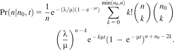If the branch length are long, that is, if then the conditional probability converges to the equilibrium distribution

For a given data set, the decay and origination parameters of the binding sites are estimated by an ML procedure by iterative hill climbing (supplementary fig. S2, Supplementary Material online). The initial step sizes are determined as ${\mathrm{\Delta }}_{\mathrm{\lambda }}=\mathrm{\lambda }/2$ and ${\mathrm{\Delta }}_{\mathrm{\mu }}=\mathrm{\mu }/2.$ Then, the likelihoods for all six combinations of parameters $({\mathrm{\lambda }}^{\prime },\mathrm{\mu }),$ $(\mathrm{\lambda },{\mathrm{\mu }}^{\prime }),$ and $({\mathrm{\lambda }}^{\prime },{\mathrm{\mu }}^{\prime })$, with ${\mathrm{\lambda }}^{\prime }=\mathrm{\lambda }\pm {\mathrm{\Delta }}_{\mathrm{\lambda }}$ and ${\mathrm{\mu }}^{\prime }=\mathrm{\mu }\pm {\mathrm{\Delta }}_{\mathrm{\mu }}$, are calculated. If the maximum of these six new likelihoods is higher than the original likelihood with parameters $(\mathrm{\lambda },\mathrm{\mu }),$ then the new parameter combination is adopted. If none of the likelihoods is higher, then the step size is reduced by a factor ½ and the likelihood evaluation is repeated. If after ten attempts to reduce the step size no improvement of L is achieved, the algorithm returns the last parameter pair as the ML estimate of the binding site turnover rates (supplementary fig. S2, Supplementary Material online). Note that for determination of step sizes for parameter optimization the evaluation of $({\mathrm{\lambda }}^{\prime },\mathrm{\mu })$ and $(\mathrm{\lambda },{\mathrm{\mu }}^{\prime })$ would be sufficient. Because the likelihoods for this model are strongly influenced by the ratio $\mathrm{\lambda }/\mathrm{\mu },$ the evaluation of likelihoods for $({\mathrm{\lambda }}^{\prime },{\mathrm{\mu }}^{\prime })$ makes the optimization more efficient.

For efficient optimization, it is also important to choose reasonable starting estimates for the turnover parameters. For this purpose, we assume that about ½ of the binding sites present at the common ancestor are still present in any two of the species sampled. The expected number of homologous binding sites is

where t is the time since the most recent common ancestor of the two species, n is the number of binding sites present in the common ancestor, and h is the number of homologous binding sites in the two species. We then have h = n/2, and we initially estimate and the origination rate from the predicted equilibrium-binding site number $\widehat{n}=\mathrm{\lambda }/\mathrm{\mu }$ as $\mathrm{\lambda }=\stackrel{-}{n}\mathrm{\mu },$ where $\stackrel{-}{n}$ is the average binding site number in the leaves for the subtree for which the parameters are estimated.

If the evolutionary distances between nodes in the tree are long compared with the half-life of the binding site, the transient probability distribution approaches the stationary distribution, which for this process is a Poisson distribution (Medhi 2003). In this case, only the ratio of the origination rate to the decay rate, $\mathrm{\lambda }/\mathrm{\mu },$ influences the likelihood and only this ratio is optimized by the program. This optimization is then preformed by keeping the original μ and only optimizing λ.

In the analysis of simulated data, we observed two kinds of situations where the optimization diverged from the true parameter values. In one case, the expected number of binding sites becomes smaller than n_min or larger than n_max. This failure can happen if origination and decay rate strongly diverge. The algorithm is failsafe, so that the optimization stops if this is happening. Another scenario we observed is that sometimes one or both parameters rapidly decrease toward zero. This zeroing happens when the binding site numbers at the leaves of the tree are too similar and thus no phylogenetic signal is present in the data. To the algorithm, this similarity indicates that the rate of binding site turnover must be very low because there is too little variation among terminal taxa.

In figure 2, the likelihood surface for the CBF1-transcription factor in our fungal data set is plotted. The likelihood function has a very distinct maximum and an extended ridge around the parameter values with the same $\mathrm{\lambda }/\mathrm{\mu }$ ratio as the ML estimates of λ and μ. This functional form demonstrates that deviations in the $\mathrm{\lambda }/\mathrm{\mu }$ ratio affect the likelihood more than individual parameter changes that leave the $\mathrm{\lambda }/\mathrm{\mu }$ ratio unaffected. We also note that the likelihood ridge levels off for larger parameter values, rather than approaching zero, such that the likelihood only depends on the $\mathrm{\lambda }/\mathrm{\mu }$ ratio and not on the individual parameters. This leveling off occurs because, as the turnover parameters increase, the estimated half-life time of a binding site decreases and the probability distribution approaches the stationary distribution, which only depends on the $\mathrm{\lambda }/\mathrm{\mu }$ ratio and not on the individual parameter values.

FIG. 2.—

Likelihood surface of the model for binding site for CBF1 in the fungal data set. The likelihood is plotted as a function of the origination rate λ and the decay rate μ of the binding sites. The likelihood function has a distinct maximum with an extended ridge (black) between the λ/μ rate corresponding to the mean binding site number (green) and the λ/μ rate corresponding to the λ/μ rate at the likelihood maximum (blue).

To estimate of confidence intervals (CIs) of the parameter estimates, we approximated the likelihood function around the optimum with the Gaussian likelihood function

where $\mathbf{v}=(\mathrm{\lambda },\mathrm{\mu })$ and ${\mathbf{v}}_O=({\mathrm{\lambda }}_{\text{opt}},{\mathrm{\mu }}_{\text{opt}})$ and C is the covariance matrix for the parameter estimates. To give a rough estimate of the CI, we use the fact that the log-Gaussian likelihood for a random variable 2 standard deviations (SDs) away from the optimum is

Hence, we find the contour line on the likelihood function that corresponds to a likelihood value of

to determine the CIs for λ and μ. The limits of the CIs are then the maximal and minimal values of which are compatible with L_confidence.

There is always a lower confidence limit as defined above, but in cases where the phylogenetic signal in the data is weak, it can happen that there is no upper confidence limit. This degenerate case occurs when the likelihood peak is higher than the ridge by less than two logL units.

Results

Simulation Results

Simulations were performed on linear and binary trees of various sizes by simulating the stochastic process of TFBS turnover (supplementary fig. S1, Supplementary Material online). That is, given a tree and the parameters of the model, the binding site number at a certain node of the tree was drawn randomly from a distribution given by the mathematical model. At the root of the tree, we assumed that the number of binding sites was equal to the equilibrium-binding site number. The randomly drawn binding site numbers at the terminal nodes of the tree were then taken as input data for the analysis by the ML algorithm described above. Simulations with different rates and clade ages were performed by setting the root node to an age of 10⁶ years and adjusting the rate parameters to obtain simulations with different relationships between clade age and turnover rate. We express the “age of the clade” in terms of relative clade age (RCA), that is, the age of the root node divided by the half-life time of the binding sites.

The Effect of Taxon Sampling

Here, we address the question how much the estimate of the model parameters is affected by the number of taxa that are included in the analysis. We first look at a set of simulations where the trees are “symmetrical,” that is, the taxa are sampled from a 16-taxon binary tree and the RCA is low, RCA = 0.5. We simulated data with 2, 3, 4, 6, 8, and 16 taxa. Trees with fewer than 16 taxa where obtained by randomly deleting taxa from a symmetrical 16-taxa tree.

The first notable trend was that there is a considerable fraction of simulations where the algorithm did not converge. On the one hand, there are the cases where the likelihood of an equilibrium model equals that of the full model taking phylogenetic structure into account. In the equilibrium model, the likelihood of any binding site number on the tree is estimated from the Poisson distribution, that is, the equilibrium distribution of the stochastic process of binding site turnover. Equilibration of binding site numbers among species can happen even in cases where the simulated clade was young compared with the half-life of binding sites and thus should not be in equilibrium. If this equilibration occurs, then it becomes impossible to estimate the individual parameters because the equilibrium distribution only depends on their ratio. Another case occurs when the parameter estimates diverged toward zero. These cases occurred for instance when, by chance, the binding site counts of taxa are too similar suggesting a low rate of evolution. Taking all these cases together (supplementary fig. S4, Supplementary Material online), the percentage of simulated data sets for which the algorithm did not converge ranged from about 30% for data with 2, 3, and 4 taxa to only 5% in the case of 16 taxa. Hence, there is a large chance (about 30%) that small data sets, that is, 4 taxa or less, cannot be analyzed because there is a high probability of a data structure that is “misleading” to the algorithm. In our simulations, however, the chance that the algorithm is not converging is only 10% with eight taxa and 5% with 16 taxa. With older clades, RCA 1 or 4, the percentage of nonconverging is larger because they are more likely to be in equilibrium (supplementary fig. S4, Supplementary Material online).

All the results discussed below are based on only those simulations where the algorithm converged, that is, the likelihood of the full model is higher than the equilibrium model and no parameter estimate diverged close to zero (optimization stops if the start parameters falls more the six orders of magnitude, typically 10⁻¹⁷ or lower, the simulated parameters are of the order of 10⁻⁵ and 10⁻⁶ for λ and μ, respectively; the estimates for these simulations are clearly distinct from the other simulations and there is no ambiguity in classifying the cases as converging or diverging).

Estimating the λ/μ Ratio from Simulated Data

Here, we consider the influence of the mean binding site number in the taxon sample on the estimated ratio of λ/μ. Remember that the ratio λ/μ predicts the expected binding site number in stochastic equilibrium. In the simulations, the root node was assigned the predicted equilibrium-binding site number, in our case 10. Nevertheless, the mean binding site number differed quite dramatically from the equilibrium expectation. In supplementary figure S5 (Supplementary Material online), we plot the minimum and the maximum mean binding site numbers, where the means are over taxa in a simulated data set and the minimum and maximum is taken over the set of simulations. Note that, even for “large” data sets with 16 taxa, the minimum mean binding site number is 7.4 and the maximum is 12; these are 20–25% different from the expectation of 10. One can expect that the algorithm would over- and underestimate λ/μ if the mean binding site number in a data set deviates strongly from the expectation. In fact, for small data sets, there is a strong correlation between the mean binding site number in a data set and the estimated λ/μ ratio. This correlation is shown in figure 3A for a sample of data sets with four taxa, where the Neyman–Pearson correlation is 0.974 and the scatter is very tight. On the other hand, in a sample of data sets with 16 taxa, the correlation is virtually zero (−0.009) (fig. 3B). Hence, with a moderately large data set, for example, 16 taxa, and a young clade (RCA = 0.5), the algorithm is able to correctly estimate the λ/μ ratio, even when the mean binding site number deviates strongly from the expected equilibrium-binding site number. Correlation coefficients between mean binding site number and estimated λ/μ ratios are given in figure 3C for data sets of 4, 6, 8, and 16 taxa, with intermediate correlations for 6 and 8 taxa. Hence, the accuracy and reliability of the estimated λ/μ ratio critically depends on the number of taxa sampled, where in young clades between 8 and 16 are sufficient. We find the same trend with linear trees, that is, trees with a pectinate structure (data not shown).

FIG. 3.—

Influence of the mean binding site number on the estimated λ/μ ratio. Although for four taxa and an RCA of 0.5 exists a strong correlation (Neyman–Pearson = 0.974) between these values (A), the correlation for 16 taxa at the same RCA is virtually 0 (Neyman–Pearson = −0.009) (B). In general, this correlation falls with rising taxa numbers and increase strongly with higher RCA (C). Because the mean binding site number tends to differ more from the equilibrium number for few taxa than for many taxa (see also supplementary fig. S5, Supplementary Material online), this suggests that λ/μ estimates are more reliable with high taxa numbers and low RCA.

We further investigated the relationship between mean binding site number and estimated λ/μ ratio for older clades with RCA of 1 and 4. In figure 3C, we also compare the correlation between mean binding site number and estimated λ/μ ratio and find that this correlation remains high even from clades with RCA = 1 and 16 taxa. It seems that the demand on data amount increases strongly with RCA so that the algorithm can estimate the correct λ/μ ratio. For instance, with a RCA of 1 and 16 data, the correlation is still 0.78 and with a RCA of 4, it is higher than 0.9.

We conclude that, with sufficient data and young enough clades, relative to the half-life of the binding site, the algorithm accurately estimates the equilibrium-binding site density for a clade, even when the mean binding site number observed is considerably different from the expectation.

Estimating the Individual Model Parameters from Simulated Data

Because the λ/μ ratio strongly influences the expected mean binding site number among taxa, this ratio is much easier to estimate than the individual parameters, λ and μ. In figure 4A and B, we plot the difference between the simulated and average estimated –log₁₀ μ and –log₁₀ λ. These data show that the average accuracy of parameter estimates can be pretty good all the way down to samples of six taxa in a clade with RCA of 0.5. Hence, there seems to be virtually no bias in the estimates. The SDs for both –log₁₀ λ as well as −log₁₀ μ estimates are pretty high, roughly around 0.3 and slightly higher for smaller data sets but generally in the same order of magnitude. Evaluation of the SDs of the estimated parameters yields CIs for these estimates. These SDs translate into factor of two differences between the estimated and the real parameters. The 95% CIs then would be compatible with roughly a 4-fold difference between estimates and true parameter values. Point estimates of binding site turnover parameters are expected to be inaccurate up to a 4-fold difference even with young clades and a moderately large taxon sample, ≤16. Estimated parameter values can thus only be considered as order of magnitude estimates.

FIG. 4.—

Influence of the number of taxa on the accuracy of the individual parameter estimates: μ (A) as well as λ (B) show relatively accurate estimates from six taxa on. For smaller taxa numbers, the predictions become more inaccurate which suggest that parameter estimation requires at least six taxa.

These trends are remarkably similar with clades of different age. For –log₁₀ λ, the average SD is 0.369 if averaged over taxa numbers and clade ages, varying between 0.49 and 0.28 if averaged over clade age and between 0.41 and 0.32 of averaged over taxa. For −log₁₀ μ, the overall average SD is 0.365 and a similar range of variation as for −log₁₀ λ. Hence, the CIs for parameter estimates are not much influenced by either taxon number or clade age. Samples with more taxa are certainly better for estimating parameters but not by much.

The Effect of Clade Age

We performed simulations of binding site turnover in clades of 16 taxa with either binary trees or linear trees. We simulated clades of different age that were composed of the same number of taxa. We express clade age in terms of RCA, that is, the age of the root node divided by the half-life time of the binding sites. We simulated clades with eight different RCAs, RCA = 0.5, 1, 1.5, 2, 3, 4, 8, and 16. In supplementary figure S6 (Supplementary Material online), we show that percent of simulations where the likelihood of the equilibrium model was less than that of the full model. This difference between likelihoods was manifested in almost all cases with young clades, that is, with an RCA of 0.5 and 1. With older clades, the fraction of nonequilibrium data sets tended to slowly decrease. It reached its lowest level of 40–60% in old clades of RCA = 16 and 16 taxa. In old clades, binary trees seem to produce a smaller fraction of nonequilibrium data sets than linear trees. This difference may occur because linear trees with the same number of taxa will have more recent nodes than in a binary tree of equally spaced internal nodes.

In figure 5, the variance/mean (V/m) ratio, that is, the ratio of the variance in binding site number across species divided by the mean binding site number, is plotted as a function of RCA. Note that for equilibrium data set, we expect V/m=1 and phylogenetic signal should lead to V/m < 1. The results for linear and binary trees are very similar, with binary trees having slightly larger average V/m for young clades. The V/m ratio starts out around 0.4 for RCA = 0.5 but quickly approaches the equilibrium value of 1 at an RCA of 3. Hence, clades which are three times as old or older than the binding site half-life are expected to approach an equilibrium value of V/m = 1.

FIG. 5.—

Influence of the RCA on the V/m ratio of the binding site numbers. Although for large RCA, the ratio corresponds to the expected equilibrium rate V/m = 1, we see for small RCA, a V/m < 1 indicating a phylogenetic signal in the data for binary (blue) as well as for linear (red) trees. Hence, clades which are at least three times as old as the binding site half-life are expected to be in equilibrium. The ratios predicted by the BOE method (yellow, see text) correspond very well with the ML estimates.

Estimates of binding site loss rate, μ, on binary trees are relatively accurate in clades of RCA up to 3 but were systematically biased upwards (fig. 6A). The bias increased approximately linearly, with a regression equation of $\mathrm{\Delta }\log \left(\mathrm{\mu }\right)=0.037\times \text{RCA}-0.023.$ In contrast, μ estimates from linear trees (fig. 6B) are accurate for RCA = 0.5 but seem to be biases toward smaller values for RCA = 1–4, on average by $\mathrm{\Delta }\log \left(\mathrm{\mu }\right)=-0.085,$ that is, the actual μ estimates are about 22% smaller than the simulated values. Above RCA = 4 the bias in μ estimates increases at $\mathrm{\Delta }\log \left(\mathrm{\mu }\right)=0.025\times \text{RCA}-0.079.$

FIG. 6.—

Influence of the RCA on the accuracy of the estimates of individual parameters. For binary trees, the estimates of μ are relatively accurate up to an RCA of 3 (A) and start then to be biased toward higher values. The estimates of λ act similarly except the negative bias at RCA 16 (C). Estimates of μ (B) and λ (D) on linear trees are similar to that on binary trees except.

For binary trees, estimates of the birth rate of binding sites, λ, are relatively accurate in the same range as the μ estimates (fig. 6C), that is, between RCA = 0.5 and 4. For RCA 4 and 8, we find a positive bias in λ estimates but with RCA = 16, a curious inversion of the trend is observed with a negative bias for λ, whereas the μ estimates have a positive bias. A similar pattern is found for linear trees (fig. 6D), except that for RCA = 1 and up to 3 the λ estimates have a negative bias. The reversion of bias in μ and λ might be related to the fact that with very old clades, the estimation essentially only estimates the V/m ratio and any stochasticity in the binding site density in terminal taxa leads to higher μ rate estimates.

Overall, these simulations show that the method performs well in estimating binding site turnover rates in young clades (RCA = 0.5) regardless of tree structure, and moderately well up to RCA = 3 for binary trees. In older clades, μ estimates seem to be systematically biased toward larger values, and λ estimates seem to have variable biases depending on RCA (see above).

A “Back of the Envelope Method” to Estimate Model Parameters

The dependency of V/m on RCA shown in figure 5 suggests that V/m follows an inverse exponential function of RCA

This functional form is reasonable, given that the effect of history decreases exponentially with time in our model (Wagner et al. 2007). In fact, the model estimating the coefficient k from the simulation data by regressing $-\ln (1-V/m)$ onto RCA gives a quite good agreement between the simulated data and the inverse exponential function (fig. 5). We simulated smaller data sets for 4 and 8 taxa to see whether the rate of increase in V/m depends on the number of taxa and found that the rate of increase is larger with more taxa than with fewer (supplementary fig. S7, Supplementary Material online). The respective regression coefficients are for 16 taxa k = 1.07, 8 taxa k = 0.81, and 4 taxa k = 0.58. The coefficient increases almost linearly with number of taxa with a regression $k=0.04\times N_{\text{taxa}}+0.45.$ Using these empirically determined relationships, we can use m, the mean binding site number, V/m ratio, and the clade age to estimate the model parameters.

Given a clade with N_taxa and clade age T_c, and with a mean binding site number of m_TF for TFBS TF and a V/m ratio substantially smaller than 1, then, we can estimate the RCA of the clade relative to this transcription factor by

From that we obtain the half-life of the TFBS using the clade age

which then relates to the decay rate of TFBSs μ by

If we assume that the mean binding site number is in equilibrium, then the origination rate λ can also be calculated

but of course, the mean binding site number does not need to be in equilibrium, and thus, this latter estimate should be considered with caution. We applied this Back Of the Envelope (BOE) method to our data and compared it with the ML estimates with relatively good results.

Application to Data

We applied the model described above to two data sets to see how the method performs on real data. The motivation for developing the method was to eventually be able to detect differences in selective constraints acting on cis-regulatory regions. Specifically, we wanted to determine whether biologically interesting patterns can be detected using this method in terms of lineage- or clade-specific differences in turnover parameters. We analyzed two data sets: one from a set of yeast genomes related to the methionine biosynthetic pathway and one from the binding sites in the mammalian HoxA gene clusters.

TFBS in the Methionine Pathway of Yeasts

The TFBS density in the 5′ region of eight single-copy genes from the methionine biosynthetic pathway was determined for 5 transcription factors and 13 species of yeasts as described above (see supplementary table 1, Supplementary Material online). Binding sites were counted from a 500 bp region upstream of each gene and the numbers in supplementary table 1 (Supplementary Material online) represent the number of binding sites per 4,000 bp (500 bp per gene) (for details, see Material and Methods). The mean binding site density, averaged over species, is highly variable, ranging from 2.7 for BAS1-binding sites to 8.1 for RTG1/3-binding sites. In order to explore the evolution of binding site density, we computed the mean binding site density and the ratio of binding site variance to mean (V/m ratio) for various clades of yeast species. According to our model, the V/m ratio is predicted to be equal to one if the binding site density distribution is in equilibrium (Wagner et al. 2007), that is, if the time of separation among the lineages is long enough to erase the phylogenetic signal. If the clade is younger, the model predicts that the V/m ratio is less than 1. If, however, the lineages are separated for a long time and differ in their expected binding site densities, the V/m ratio can be larger than 1. With these criteria in mind, we can perform an exploratory analysis of our data.

Figure 7 shows the relationship of the V/m ratio over the estimated age of the clade. In the youngest clade, clade F in figure 8A–E, of 4 species most closely related to S. cerevisiae (about 20 My), the V/m ratio for all five binding sites is less than 1 (P = 0.0125, sign test) and two binding sites individually have a V/m ration significantly less than 1 (CBF1, P = 0.032; GCN4, P = 0.039). For older clades, the V/m ratio tends to be larger but with considerable variation among binding site classes, roughly consistent with the expectation of the model. In all binding site classes, the count of binding sites in S. pombe is low and will be excluded from further analysis. Below, we summarize the variation in binding site density for individual binding site classes.

FIG. 7.—

Relationship of the RCA and the V/m ratio of binding sites of the transcription factors in the methionine pathway of yeast. The letters in the graph refer to the clade labels in figure 8. Whereas for the youngest clade F the V/m ratios for all transcription factors are less than 1, the ratios tends to be large for older clades but still have a considerable variation among binding site classes. Note that V/m ratios larger than 1 suggest heterogeneity of binding site number among taxa.

FIG. 8.—

Evolution of binding site number for transcription factors in the methionine pathway of yeast. Clades are marked by a letter at their root and a bracket with the mean binding site number and the V/m ratio above the corresponding species names. For some species the binding site numbers are also given above the name. The whole-genome duplication of the E clade is marked by WGD. For CBF1 (A), the likelihood model estimates a half-life of 57.3 My. There also seems to be a significant decrease in the binding site density in stem lineage of the G clade. GCN4 (B) has with 84.1 My, the longest estimated half-life and a significant loss of binding sites in the D clade. MET30/31 (C) has an estimated half-life of 24.2 My and like CBF1 a significant binding site loss in the G clade. BAS1 (D) has an estimated half-life of 22.7 My. RTG1/3 (E) has in the F clade a V/m ratio close to 1 (0.84), suggesting equilibrium within the 20 Mio years time frame of the F clade. This makes the estimation of the rate parameters difficult and yields to the shortest half-life of only 30.900 years.

CBF1-binding site density in the A clade (i.e., all species except S. pombe) is 7.3 (fig. 8A). The V/m ratio in the A clade is significantly elevated above 1 (V/m = 2.26, P = 0.012) and thus indicates heterogeneity in average binding site density among lineages. This heterogeneity arises from differences among the C clade and its two outgroup clades, clade G and Y. lipolytica (fig. 8A). The C clade itself has a V/m ratio of 1.78, which is not significantly elevated above one (P = 0.30). Within the C clade, the youngest clade F has a significantly decreased V/m ratio of 0.09 (P = 0.032). This indicates that the half-life of the CBF1-binding sites is longer than the age of the F clade. Estimating the half-life with the likelihood model yields a value of 57.3 Mio years, which is almost three times the age of F clade, about 19.8 Mio years. Comparing the binding site densities in the G clade (1.5), the direct outgroup of C, suggests that binding site density might have been decreased in the stem lineage of the G clade. A likelihood ratio test (LRT) using our model suggests that this rate difference is significant (χ² = 11.05; P = 0.004, 2 degrees of freedom [df]). The ML-estimated CBF1-binding site origination rate is 0.02 binding sites/kb × Mio years.

The average density of GCN4-binding sites is 6.4 and has only a slightly elevated V/m ratio of 1.6 (P = 0.09) (fig. 8B). In contrast, the C clade has significant heterogeneity as indicated by a V/m ratio of 1.96 (P = 0.047), which is caused by a lower binding site density in the D clade (mean = 2.3, V/m = 1.0) than in the E clade (mean = 8.2, V/m = 0.61; P = 0.31). The outgroups of the C clade, G clade, and Y. lipolytica are more similar to the E clade (combined mean = 7.0, V/m = 1.0) suggesting that the D clade lost GCN4-binding sites in evolution. This inference is supported by a LRT with our model (χ² = 9.29; P = 0.0096, 2 df). GCN4 has the longest estimated half-life among the binding sites investigated here, 84.1 Mio years, and a slightly lower than average origination rate of 0.013/kb × Mio years.

Over all species (except S. pombe), the binding site density for MET30/31 is 5.8 and heterogeneous, with a significantly elevated V/m ratio of 2.98 (P = 5.8 10⁻⁴) (fig. 8C). The heterogeneity is caused by a difference between the binding site densities in the C clade, which has a mean of 5.7 and a V/m ratio of 0.84, and the two outgroups. The first outgroup, the G clade has a much lower binding site density of 1 and Y. lipolytica an elevated binding site density of 16. Testing for a decreased binding site density with our likelihood model supports the inference that the G clade has a lower equilibrium density (χ² = 13.02; P = 0.0015, 2 df). The C clade itself seems to be homogenous (P = 0.43). The half-life of MET30/31-binding sites is relatively short, at 24.2 Mio years, and the origination rate is 0.034 binding sites/kb × Mio years.

The binding site density for BAS1 is low, with an average of 2.69 and ranging from 0 in S. pombe to a maximum of 5 (fig. 8D). In general, mean binding site density is similar among clades and the V/m ratio generally remains below one. There is no particular pattern to binding site density differences. The estimated rate parameters are 0.02 binding sites originating per kb and 1 Mio years, the half-life for a BAS1-binding site is estimated to be 22.7 Mio years.

The average binding site density of RTG1/3 in the A clade is 8.6 and highly heterogeneous, V/m = 2.76 (P = 1.4 × 10⁻³) (fig. 8E). The heterogeneity arises at various levels. As for MET30/31, the density is high in Y. lipolytica (m = 15) and depressed in the G clade (m = 4). Also, the C clade is heterogeneous with a mean of 9.0 and a V/m ratio of 2.25 (P = 0.021). The heterogeneity in the C clade is caused by heterogeneity in the D clade, which has a mean of 10 and a V/m ratio of 4.3 (P = 0.014), where the densities range from 17 to 4. ML estimates of the rate parameters are not possible with accuracy because the reconstructions suggest that the process quickly equilibrates, which only makes the ratio of rate parameters determined by data. This observation is consistent with the relatively high V/m ratio of 0.84 among the species of the F clade, the youngest clade in our taxon sample. This V/m ratio is not significantly different from 1 suggesting equilibration within the 20 Mio time frame of the F clade. Using the BOE method sketched above (which does not depend on the convergence of the likelihood algorithm), just based on the V/m ratio, suggests a half-life of only 6.2 × 10⁶ and an origination rate as high as 0.21 binding site per kb and Mio years.

Estimated Rates of Binding Site Origination and Decay in Yeasts

Comparing the data among binding site types suggests that binding site densities come in two modes. One mode ranges from 5 to 10 sites and the other consisted of lineages have binding site densities of 1–2. Given that binding sites were sampled from the 5′ region of eight genes, binding site densities of about 1–2 probably represent spurious binding site distributions, suggesting that this transcription factor is not functional in the methionine pathway of the respective species. If this interpretation is correct, it seems that certain transcription factors have been replaced in some clades, often in the G clade, by some other transcription factor, as has been demonstrated for the ribosomal protein module (Tuch et al. 2008). This scenario seems to apply to RTG1/3, MET30/31, and CBF1 in the G clade, represented here by D. hansenii and C. albicans. A similar drop in binding site density happened in the D clade, represented by A. gossypii, K. lactis, and K. waltii, for the GCN4-binding sites. These inferences from the binding site density patterns predict a shift in the functional role of the respective transcription factors. Another possibility is that in this clade, the binding site motifs and the transcription factor DNA–binding specificity has changed; thus, the TFBSs are no longer recognizable.

We compared the ML and the BOE estimates of the model parameters (supplementary fig. S8A–D, Supplementary Material online). The ML estimates use an explicit likelihood framework to estimate parameters for a given phylogeny, whereas the BOE method only uses empirical relationships between V/m and RCA, determined by simulation, to estimate parameters. Given the difficulties of estimating these parameters, the correlation between the ML and BOE estimates of μ are quite reasonable (r² = 0.764 excluding RTG1/3, which inflates the correlation, supplementary fig. S8A and B, Supplementary Material online). In contrast, the λ estimates have a low correlation of 0.392 (excluding MET30/31, which is an outlier) (supplementary fig. S8C and D, Supplementary Material online). However, the three binding site origination rate estimates for CBF1, BAS1, and GCN4 are close to the line where the BOE and ML rate are equal (supplementary fig. S8D, Supplementary Material online).

TFBS in Vertebrate HoxA Cluster

The binding site density in the vertebrate HoxA clusters was determined from ∼150 kb of genomic sequence and from 20 species (see supplementary table 2, Supplementary Material online). Specifically, we investigated the binding site for the estrogen receptor (ERE), the progesterone receptor (PRE), and the retinoic acid receptor (RARE).

In the total data set, containing 15 mammalian species and 5 nonmammalian species, the steroid-response elements (SRE = either PRE or ERE) are significantly overdispersed, suggesting heterogeneity among lineages in terms of the PRE and ERE density (fig. 9A–C). Specifically, the V/m ratio for PRE is 1.73 (P = 0.025) and for ERE 1.86 (P = 0.013). This heterogeneity is caused by a difference between the mammalian and the nonmammalian taxa. The mammalian clade has higher SRE densities (PRE mean = 10.8, ERE mean = 11.2) than the nonmammalian species (PRE mean = 5.8, ERE mean = 5.2). The mammalian clade shows no evidence of heterogeneity (PRE V/m = 0.97; ERE V/m = 0.64, P = 0.17). This suggests that the SREs experienced a 2-fold increase in equilibrium density from about 5 to about 10. The LRT using our model supports this conclusion (PRE χ² = 17.67, P = 1.46 × 10⁻⁴, 2 df; ERE × χ² = 22.72, P = 1.16 × 10⁻⁵, 2 df).

FIG. 9.—

Evolution of binding site numbers in the HoxA clusters of vertebrates. Clades are marked by a bracket with the mean binding site number and the V/m ratio above the corresponding species names. The binding site numbers of PRE (A) and ERE (B) are significantly overdispersed caused by differences between the mammalian and nonmammalian taxa. The mammalian clade shows no evidence of heterogeneity (V/m of PRE = 0.97, V/m of ERE = 0.64), which suggests a 2-fold increase in equilibrium density from about 5–10. The P value at the stem lineage of the mammalian clade are those of the LRT showing that the mammalian and the nonmammalian lineages have different turnover rates and equilibrium densities of PRE and ERE. RARE (C) show a very low density and variation with a V/m ratio of 0.47 suggesting a low turnover rate. There is also no evidence for heterogeneity which is consistent with the ancestral and conserved function of RARE.

The density of RARE elements is low compared with that of the SRE, with an overall mean of 3.5. The variation of RARE density is also low, with an overall V/m ratio of 0.47 (P = 0.024), suggesting that RARE have a lower turnover rate than SRE. No evidence of heterogeneity has been found in this data set, consistent with the ancestral function of RARE in Hox gene regulation.

The estimated half-life for SREs is similar, about 10 Mio years based on ML estimates (PRE T_1/2 = 11.7 Mio years; ERE T_1/2 = 7.23 Mio years). We chose the primate clade to do a BOE estimate for ERE, which yields a half-life for ERE of 22.7 Mio years. Within the mammals, the PRE seem to be in equilibrium in even the most recent clade with at least four species, that is, the tamarin, macaque, chimp, and human (V/m = 1.6, P = 0.19). This clade has an estimated age of 43 Mio years and thus the BOE estimate of half-life time is likely to be less than 10 Mio years, that is, this clade would have an RCA of 4 or higher, based on the simulation results with four taxa. This RCA is consistent with the ML likelihood estimate of 7.23 Mio years.

The half-life estimates for SREs are of the same order of magnitude as those for TFBSs in yeast (20–80 Mio years), but on the lower end of that distribution. As expected from the V/m ratios, the half-life time of the RARE is estimated to be longer than that of SRE, T_1/2 = 147 Mio years, which is 1 order of magnitude higher than for SRE. This probably reflects stronger selection against changes in RARE elements because of their central role in vertebrate development. A BOE estimate using the data from the eutherian clade yields T_1/2 = 289 Mio years, which is a factor two higher than the ML estimate but still in the same order of magnitude.

The origination rates for the SREs are 0.005/(kb × Mio years) and 0.008/(kb × Mio years) for PRE and ERE, respectively. In contrast, the origination rate for RARE is only 0.0001/(kb × Mio years). There is a general negative relationship between origination rates and half-life times such that the shorter the half-life time, the higher the origination rate (see also the results for yeast-binding sites). Such a negative relationship can be explained if we assume that binding site turnover is due to accidental fixation of slightly deleterious mutations and the selection of compensatory mutations. In equilibrium then, the origination rate is driven by the accidental loss rate, which in turn is determined by the population size and the intensity of stabilizing selection on the binding sites. The stronger the selection, the lower is the fixation probability of deleterious mutations. As a consequence, the smaller is the need for the fixation of compensatory mutations.

Discussion

In this paper, we explored the utility of a phenomenological mathematical model of binding site turnover (Wagner et al. 2007) for the analysis of CRE evolution. Specifically, we wanted to determine whether this model could guide investigators in identifying clades where the selective forces acting on binding sites in CREs are different. We assume that, in the case of poorly conserved but functionally important TFBSs, selection primarily affects the rate of TFBS turnover and thus leads to differences in average binding site density between lineages. Here, we show that the predictions of the model can be used in two ways. On the one hand, the model can be used for exploratory “BOE” data analysis. On the other hand, the ML implementation of the model can be used to estimate model parameters and in LRTs for differences in turnover rates between clades. The latter test is a key tool for identifying functionally important changes in the evolution of cis-regulation.

The exploratory data analysis using this model is based on the prediction that in stochastic equilibrium, the ratio of variance to mean is equal to 1, V/m = 1. The data analyzed here is qualitatively consistent with this prediction as younger clades tend to have V/m ratios smaller than 1 and older clades tend to have V/m ratios around 1. In the case of V/m > 1, the model predicts that there should be heterogeneity in binding site density among lineages. This is often the case in the data sets we analyzed as clear instances of heterogeneity of mean binding site density are identifiable in clades with V/m > 1 (see figs. 8 and 9). LRTs for heterogeneity in the rate of binding site turnover confirm this inference. Hence, comparing V/m ratios between clades can be used as a useful heuristic to identify homogenous binding site dynamics and infer variation in selective constraints acting on TFBSs.

The ML method described here is most useful for testing for heterogeneity in the turnover rate and thus testing for differences in the selective constraints on TFBSs. For example, we found that PRE and ERE densities in HoxA clusters are heterogeneous among gnathostomes, comparison of V/m ratios, and mean binding site densities indicate that the heterogeneity is between mammals and the other gnathostomes. The ERE and PRE densities in mammals are about twice that observed in nonmammalian. A LRT test indicated that these differences are highly significant (PRE: P = 1.4 × 10⁻⁴; ERE: P = 1.2 × 10⁻⁵), suggesting a greater involvement of HoxA genes in female reproductive function in mammals than in nonmammalian gnathostomes. Indeed, in humans and other placental mammals, HoxA-13, HoxA-11, HoxA-10, and HoxA-9 have been shown to be involved in female fertility and development of the reproductive tract and mammary gland and directly responsive to hormone signaling (Daftary and Taylor 2006). Unexpectedly, ERE and PRE density increased in the stem lineage of mammals rather than in the therian or eutherian stem lineage coincident with the evolution of internal development and placentation, respectively. A possible explanation of the early increase SREs is the involvement of HoxA-9 and HoxA-5 in mammary gland development and function (Chen and Capecchi 1999), which evolved in the stem lineage of mammals. This apparent increase in involvement of steroids in regulating Hox genes might have been preadaptive (exaptive) for the later evolving role of HoxA-11 in placental function (Lynch et al. 2008). In contrast, there was no heterogeneity in RARE density among the gnathostome taxa sampled, which is consistent with the ancient and conserved role of retinoid acid in Hox gene regulation.

In our yeast data set, heterogeneity in binding site density is most often associated with a decrease in density in the clade including C. albicans. We find this reduced density for CBF1- and MET30/31-binding sites (clade G in fig. 8A and C), suggesting that these transcription factors play a diminished role in regulating the methionine pathway genes in these species. A similar pattern applies to GCN4-binding sites in the clade including K. lactis (clade D in fig. 8B). It would be interesting to test for the function of these transcription factors in methionine biosynthesis in these species.

Estimates of the model parameters are imprecise in our data, at least as judged by CIs derived from the likelihood functions, suggesting that dense taxon sampling is required for more precise parameter estimation. Indeed, our data indicate that larger taxon sampling in younger clades is necessary to obtain more accurate estimates. Even with these caveats, however, several general trends in binding site turnover are apparent. For example, the half-life of a “typical” TFBS is between 10 and 100 Mio years, whereas more constrained binding sites, such as RAREs in mammalian HoxA clusters, have an estimated half-life time of about 150 Mio years. At the lower end of the half-life time, distribution are EREs in the mammalian HoxA clusters with an estimated half-life time of about 7 My. This indicates that the optimal taxon sampling and phylogenetic depth needed for accurate inferences in binding site density dynamics is variable, such that more constrained sites require deeper taxon sampling, whereas binding site sites with higher turnover rates require dense sampling of younger clades. Based on our simulation results, we recommend studies of binding site dynamics should include at least six species (fig. 4A and B), although the choice of taxon sampling depends heavily on half-life of the binding site in that clade. In studies of genomic regions from species that are closely related, one also has the added benefit that the number of orthologous binding sites could be determined by sequence alignment, which will further increase the accuracy of the parameter estimates (Wagner et al. 2007).

Overall, our results show that an ML implementation of the stochastic binding site turnover model of Wagner et al. (2007) allows for the analysis of binding site density in an explicit phylogenetic context. The model can be used to statistically test for relative differences in the turnover rate and equilibrium density of TFBSs as well as gain insights into the actual rate of binding site turnover. The development of this and other models of TFBS evolution has the potential to reveal the rate and pattern of CRE evolution similar to the development of codon-based models of protein evolution.

Supplementary Material

Supplementary figures S1–S8 and tables 1 and 2 are available at Genome Biology and Evolution online (http://www.oxfordjournals.org/our_journals/gbe/).

Funding

This work was supported by a Research Prize from the Alexander von Humboldt Foundation [to G.P.W.]; the work in the Wagner lab was supported by the John Templeton Foundation [grant # 12793]; the Konrad Adenauer Foundation and the International Max Planck Research School “Mathematics in the Sciences” [W.O.]; the postdoctoral program “Beatriu de Pinós” from the Departament d'Universitats, Recerca i Societat de la Informació, Generalitat de Catalunya (ref. 2006 BP-A 10081 to F.L.-G.).

References

- Akbas GE, Song J, Taylor HS. A HOXA10 estrogen response element (ERE) is differentially regulated by 17 beta-estradiol and diethylstilbestrol (DES) J Mol Biol. 2004;340(5):1013–1023. doi: 10.1016/j.jmb.2004.05.052. [DOI] [PubMed] [Google Scholar]
- Balhoff JP, Wray GA. Evolutionary analysis of the well characterized endo16 promoter reveals substantial variation within functional sites. Proc Natl Acad Sci USA. 2005;102(24):8591–8596. doi: 10.1073/pnas.0409638102. [DOI] [PMC free article] [PubMed] [Google Scholar]
- Bourdeau V, et al. Genome-wide identification of high-affinity estrogen response elements in human and mouse. Mol Endocrinol. 2004;18(6):1411–1427. doi: 10.1210/me.2003-0441. [DOI] [PubMed] [Google Scholar]
- Chen F, Capecchi MR. Paralogous mouse Hox genes, Hoxa9, Hoxb9, and Hoxd9, function together to control development of the mammary gland in response to pregnancy. Proc Natl Acad Sci USA. 1999;96(2):541–546. doi: 10.1073/pnas.96.2.541. [DOI] [PMC free article] [PubMed] [Google Scholar]
- Crocker J, Erives A. A closer look at the eve stripe 2 enhancers of Drosophila and Themira. PLoS Genet. 2008;4(11):e1000276. doi: 10.1371/journal.pgen.1000276. [DOI] [PMC free article] [PubMed] [Google Scholar]
- Daftary GS, Taylor HS. Endocrine regulation of HOX genes. Endocr Rev. 2006;27(4):331–55. doi: 10.1210/er.2005-0018. [DOI] [PubMed] [Google Scholar]
- Gasch AP, et al. Conservation and evolution of cis-regulatory systems in ascomycete fungi. PLoS Biol. 2004;2(12):e398. doi: 10.1371/journal.pbio.0020398. [DOI] [PMC free article] [PubMed] [Google Scholar]
- Gompel N, Prud'homme B, Wittkopp PJ, Kassner VA, Carroll SB. Chance caught on the wing: cis-regulatory evolution and the origin of pigment patterns in Drosophila. Nature. 2005;433:481–487. doi: 10.1038/nature03235. [DOI] [PubMed] [Google Scholar]
- Haygood R, Fedrigo O, Hanson B, Yokoyama KD, Wray GA. Promoter regions of many neural- and nutrition-related genes have experienced positive selection during human evolution. Nat Genet. 2007;39(9):1140–1144. doi: 10.1038/ng2104. [DOI] [PubMed] [Google Scholar]
- Istrail S, Davidson EH. Logic functions of the genomic cis-regulatory code. Proc Natl Acad Sci USA. 2005;102:4954–4959. doi: 10.1073/pnas.0409624102. [DOI] [PMC free article] [PubMed] [Google Scholar]
- Lynch VJ, Tanzer A. Adaptive changes in the transcription factor HoxA-11 are essential for the evolution of pregnancy in mammals. Proc Natl Acad Sci USA. 2008;105(39):14928–14933. doi: 10.1073/pnas.0802355105. [DOI] [PMC free article] [PubMed] [Google Scholar]
- Mainguy G, et al. A position-dependent organisation of retinoid response elements is conserved in the vertebrate Hox clusters. Trends Genet. 2003;19(9):476–479. doi: 10.1016/S0168-9525(03)00202-6. [DOI] [PubMed] [Google Scholar]
- Medhi J. Stochastic models in queueing theory. Amsterdam: Academic Press; 2003. [Google Scholar]
- Miranda I, Silva R, Santos MA. Evolution of the genetic code in yeasts. Yeast. 2006;23(3):203–213. doi: 10.1002/yea.1350. [DOI] [PubMed] [Google Scholar]
- Nelson CC, et al. Determinants of DNA sequence specificity of the androgen, progesterone, and glucocorticoid receptors: evidence for differential receptor response elements. Mol Endocrinol. 1999;13(12):2090–2107. doi: 10.1210/mend.13.12.0396. [DOI] [PubMed] [Google Scholar]
- Prabhakar S, Noonan JP, Pääbo S, Rubin EM. Accelerated evolution of conserved noncoding sequences in humans. Science. 2006;314(5800):786. doi: 10.1126/science.1130738. [DOI] [PubMed] [Google Scholar]
- Sanderson M. Analysis of rates (”r8s”) of evolution. 2006. [Internet]. [cited 2009 June 15]. Available from http://loco.biosci.arizona.edu/r8s/ [Google Scholar]
- Tuch BB, Galgoczy DJ, Hernday AD, Li H, Johnson AD. The evolution of combinatorial gene regulation in fungi. PLoS Biol. 2008;6(2):e38. doi: 10.1371/journal.pbio.0060038. [DOI] [PMC free article] [PubMed] [Google Scholar]
- Wagner GP, Fried C, Prohaska SJ, Stadler PF. Divergence of conserved non-coding sequences: rate estimates and relative rate tests. Mol Biol Evol. 2004;21:2116–2121. doi: 10.1093/molbev/msh221. [DOI] [PubMed] [Google Scholar]
- Wagner GP, Lynch VJ. The gene regulatory logic of transcription factor evolution. Trends Ecol Evol. 2008;23(7):377–385. doi: 10.1016/j.tree.2008.03.006. [DOI] [PubMed] [Google Scholar]
- Wagner GP, Otto W, Lynch V, Stadler PF. A stochastic model for the evolution of transcription factor binding site abundance. J Theor Biol. 2007;247:544–553. doi: 10.1016/j.jtbi.2007.03.001. [DOI] [PubMed] [Google Scholar]
- Wapinski I, Pfeffer A, Friedman N, Regev A. Natural history and evolutionary principles of gene duplication in fungi. Nature. 2007;449(7158):54–61. doi: 10.1038/nature06107. [DOI] [PubMed] [Google Scholar]
- Wong WSW, Nielsen R. Detecting selection in non-coding regions of nucleotide sequences. Genetics. 2004;167:949–958. doi: 10.1534/genetics.102.010959. [DOI] [PMC free article] [PubMed] [Google Scholar]
- Wray GA. Resolving the Hox paradox. Science. 2001;292:2257. [Google Scholar]
Associated Data
This section collects any data citations, data availability statements, or supplementary materials included in this article.