A Modified Fuzzy C-Means Classification Method Using a Multiscale Diffusion Filtering Scheme

Abstract

A fully automatic, multiscale fuzzy c-means (MsFCM) classification method for MR images is presented in this paper. We use a diffusion filter to process MR images and to construct a multiscale image series. A multiscale fuzzy C-means classification method is applied along the scales from the coarse to fine levels. The objective function of the conventional fuzzy c-means (FCM) method is modified to allow multiscale classification processing where the result from a coarse scale supervises the classification in the next fine scale. The method is robust for noise and low-contrast MR images because of its multiscale diffusion filtering scheme. The new method was compared with the conventional FCM method and a modified FCM (MFCM) method. Validation studies were performed on synthesized images with various contrasts and on the McGill brain MR image database. Our MsFCM method consistently performed better than the conventional FCM and MFCM methods. The MsFCM method achieved an overlap ratio of greater than 90% as validated by the ground truth. Experiments results on real MR images were given to demonstrate the effectiveness of the proposed method. Our multiscale fuzzy c-means classification method is accurate and robust for various MR images. It can provide a quantitative tool for neuroimaging and other applications.

1. Introduction

Magnetic resonance imaging (MRI) can provide unique tissue contrasts such as diffusion weighted imaging and quantitative T1, T2 measurements, which are promising as in vivo imaging markers that can detect early therapeutic response of tumors to therapy (Carano et al., 2004; Jacobs et al., 2001; Li et al., 2005). Image classification is an important step for quantitative analysis in order to detect pathology or quantify disease response to therapy.

Image classification is a process to partition an image into a set of distinct classes with uniform or homogeneous attributes such as textures or intensity. Classification methods can be categorized as supervised and unsupervised methods (James, 1985; Lu and Weng, 2007). Supervised classification methods depend on the examples of information classes in the images and derive a prior model or parameters from the training sets (Cocosco et al., 2003). Unsupervised methods examine the images without specific training data and divide the image pixels into groups presented in the pixel values according to classification criteria. Unsupervised methods have the advantage of being fast and not requiring training information which is sometimes unavailable (Young et al., 1986).

Classification of MR images can be challenging because they can be affected by multiple factors such as noise, poor contrast, intensity inhomogeneity, or partial volume effects. Partial volume effects occur where pixels contain a mixture of multiple tissue types, thus making it difficult to assign a single class to the boundary regions. The conventional ‘hard’ classification method restricts each pixel exclusively to one class and often results in a very crisp result; therefore, fuzzy classification or “soft” segmentation has been extensively applied to MR images in which pixels are partially classified into multiple classes.

A variety of fuzzy classification methods have been reported. First, statistical model-based methods have been used for quantification of brain tissues in MR images (Cuadra et al., 2005; Van Leemput et al., 1999). These methods typically employ a Gaussian finite mixture model to estimate the class mixture of each pixel by trying to fit the image histogram. The intensity of a single tissue type is modeled as a Gaussian distribution, and the classification problem is solved by using the expectation-maximization (EM) algorithm (Marroquin et al., 2002). Because of partial volume effects and intratumor heterogeneity, the intensity distribution may deviate from the Gaussian model. The intrinsic limitation of this method is that it assumes the independence of all the pixel intensity values and that it fails to take into account the spatial correlation between pixels. Such a limitation might cause this method to be sensitive to noise and thus to produce unreliable results for MR images (Choi et al., 1991). Markov random field (MRF) is developed to model the spatial correlation and is used as prior information in the EM optimization (Held et al., 1997; Zhang et al., 2001). However, it is difficult to estimate parameters for an MRF model from the images. Meanwhile, as the MRF-EM method is computationally intensive and could easily be trapped into a local minimum, a good initial guess regarding tissue clustering is highly needed.

Second, fuzzy c-means (FCM) classification methods employ fuzzy partitioning and allow one pixel to belong to tissue types with different membership graded between 0 and 1 (Bezdek, 1980). FCM is an unsupervised algorithm which allows soft classification of each pixel which possibly consists of several different tissue types (Pham and Prince, 1999). Although the conventional FCM algorithm works well on most noise-free images, it does not incorporate the spatial correlation information which would cause it to be sensitive to noise and MR inhomogeneity. A different, modified FCM has been proposed to compensate for MR field inhomogeneity and to incorporate the spatial information. Tolias and Panas (1998) imposed the spatial continuity constraints by post-processing the results obtained from conventional FCM classification where a set of rules describing regional homogeneity were applied to update the fuzzy membership. A geometry-guided FCM (GC-FCM) method was proposed by Noordam et al. (2000) where local neighborhood information was incorporated into the optimization process. Recently, some approaches directly added regularization terms to the objective function, thereby showing increased robustness of the classification to noisy images. A regularization term has been introduced into the conventional FCM cost function in order to impose a neighborhood effect (Ahmed et al., 2002). A pixel is likely to be the same class if the majority of neighborhood pixels belong to one class. In this way, the final solution is guided to a piecewise-homogeneous clustering. This method was demonstrated to be useful for MR images corrupted by salt and pepper noise. Inspired by the Markov random field and expectation-maximization algorithm (Zhang, Y. et al., 2001), various modified FCM methods were proposed incorporating different regularization terms to overcome the noise sensitivity of FCM (Chen and Zhang, 2004; Liew and Yan, 2003). These regularizations penalized the FCM cost function using the spatial dependence between neighboring pixels. However, high-level spatial information other than neighboring pixels could be useful for classification. Similar to the statistical model-based methods as mentioned above, these FCM methods are computationally expensive, especially for multispectral 3D MR volumes. An FCM method also depends on the initial guess which greatly affects the speed and stability of the classification.

In this study, we propose a new, fully automatic, multiscale fuzzy c-means (MsFCM) classification method for MR images. We use a diffusion filter to smooth the MR images and to construct multiscale image series. A multiscale fuzzy C-means classification method is applied along the scales from coarse to fine levels. The objective function of the conventional FCM is modified to allow multiscale classification processing where the result from a coarse scale supervises the classification of the next fine scale. The multiscale fuzzy c-means (MsFCM) classification is described in the following section. Results on synthetic data and real MR images are reported.

2. Classification Method

2.1 Multiscale space from anisotropic diffusion filtering

As image classification algorithms can be sensitive to noise, image filtering can improve the performance of classification. Due to partial volume effect, MR images often have blurred edges. Linear low-pass filtering gives poor results as it incurs even more edge blurring and detail loss. Anisotropic diffusion filtering can overcome this drawback by introducing a partial edge detection step into the filtering process so as to encourage intra-region smoothing and preserve the inter-region edge. Anisotropic diffusion filtering, introduced by Perona and Malik (Perona and Malik, 1990), is a partial differential diffusion equation model described as

$$\frac{\partial x(i,t)}{\partial t}=\mathit{div}(c(x_i,t)\nabla x(i,t))$$ (1)

x_i is the MR image intensity at the position i, x(i,t) stands for the intensity at the position i and the time t or the scale level t; ∇ and div are the spatial gradient and divergence operator. c(x_i, t) is the diffusion coefficient and is chosen locally as a function of the magnitude of the image intensity gradient

$$c(x_i,t)=e^{-{(\parallel \nabla x(i,t)\parallel ∕\omega )}^2}$$ (2)

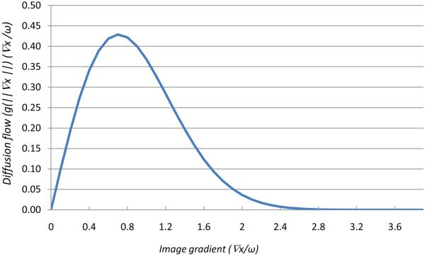
The constant ω is referred as the diffusion constant and determines the filtering behavior. As shown in Fig. 1, the local flow function Φ(x_i,t) = c(x_i,t)∇x(i,t) is plotted as a function of the diffusion constant. Maximal flow presents where the gradient strength is equal to the diffusion constant (∇x ≈ ω); the flow rapidly decreases to zero when the gradient is close to zero or much greater than ω, which implies that the diffusion process maintains a homogeneous region (where ∇x ⪡ ω) and preserves edges where ∇x ⪢ ω. To reduce noise in the image, ω is chosen as the gradient magnitude produced by noise and is generally fixed manually or estimated using the noise estimator described by Canny (1986).

Fig.1.

Mechanism of a diffusion filter for removing noise and preserving edges. Diffusion flow (Y-axis) is plotted as a function of image gradients (X-axis). When the gradient ∇I is close to zero (homogeneity regions) or when the flow is much greater than k (the edges), the flow rapidly decreases to zero which indicates no filtering processing. This implies that the diffusion filter processing maintains a homogeneous region and preserves edge information. The flow is maximum when the gradient strength is near to the diffusion constant k. To reduce noise in the image, k is carefully chosen so that the flow is maximum and the filter will remove the noise at that gradient.

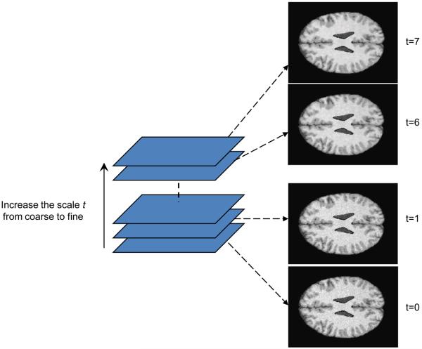
The multiscale approach represents a series of images with different levels of spatial resolution. General information is extracted and maintained in large-scale images, and low-scale images have more local tissue information. The multiscale approach can effectively improve the classification speed and can avoid trapping into local solutions. Anisotropic diffusion is a scale space, adaptive technique which iteratively smoothes the images as the time t increases. Our multiscale description of images is generated by the anisotropic diffusion filter. The time t is considered as the scale level and the original image is at the level 0. When the scale increases, the images become more blurred and contain more general information. Fig. 2 illustrates the scale space which was constructed using anisotropic diffusion filtering. Unlike many multi-resolution techniques where the images are down-sampled along the resolution, we kept the image resolution along the scales.

Fig.2.

Scale-space constructed by anisotropic diffusion filtering. The scale space is composed of a stack of the images filtered at different scales where t=0 is the original image. The greater the scale level, the less local information appears.

2.2 Conventional Fuzzy C-Means (FCM) Method

The conventional fuzzy c-means (FCM) algorithm is an iterative method that produces optimal c partitions for the image ${\left\{x_i\right\}}_{i=1}^N$ by minimizing the weighted inter-group sum of the squared error objective function J_FCM

$$J_{\mathit{FCM}}=\underset{k=1}{\overset{c}{\Sigma }}\underset{i=1}{\overset{N}{\Sigma }}{u}_{\mathit{ik}}^p{\Vert x_i-v_k\Vert }^2$$ (3)

Where ${\left\{v_k\right\}}_{k=1}^c$ is the characterized intensity center of the class k and c is the number of underlying tissue types in the images. u_ik represents the possibility of the pixel i belonging to the class k and requires u_ik ∈[0,1] and ${\displaystyle {\Sigma }_{k=1}^c}{u}_{\mathit{ik}}=1$ for any pixel i. The parameter p is a weighting exponent on each fuzzy membership and is set as 2.

As the FCM objective function is minimized, each pixel is assigned a high membership in a class whose center is close to the intensity of the pixel. A low membership is given when the pixel intensity is far from the class centroid. The FCM is minimized when the first derivatives of Equation (3) with respect to u_ik and v_k are zero. The final classes and their centers are computed iteratively through these two necessary conditions. In the end, a hard classification is reached by assigning each pixel solely to the class with the highest membership value.

2.3 Modified fuzzy C-means (MFCM) method

A conventional FCM method only uses pixel intensity information and results in crisp segmentation for noisy images. In order to incorporate spatial information, different modified fuzzy c-means methods are proposed to allow the neighbors as factors and thus to attract pixels into their cluster. The modified fuzzy c-means method (MFCM) proposed by (Ahmed et al., 2002) has an objective function

$$J=\underset{k=1}{\overset{c}{\Sigma }}\underset{i=1}{\overset{N}{\Sigma }}{u}_{\mathit{ik}}^p{\Vert x_i-v_k\Vert }^2+\frac{\alpha }{N_R}\underset{k=1}{\overset{c}{\Sigma }}\underset{i=1}{\overset{N}{\Sigma }}{u}_{\mathit{ik}}^p\left(\underset{x_r\in N_i}{\Sigma }{\Vert x_r-v_k\Vert }^2\right)$$ (4)

Where N_i stands for the neighboring pixels of the pixel i and N_R is the total number of neighboring pixels, which is 8 for a 2D image and 26 for a 3D volume. α controls the effect of the neighboring term and is inversely proportional to the signal-to-noise (SNR) levels of the MR images.

2.4 Multiscale Fuzzy C-means (MsFCM) algorithm

After anisotropic diffusion filtering processing, our multiscale Fuzzy C-means algorithm (MsFCM) performs classification from the coarsest to the finest scale, i.e. the original image. The classification result at a coarser level t+1 was used to initialize the classification at a higher scale level t. The final classification is the result at the scale level 0. During the classification processing at the level t+1, the pixels with the highest membership above a threshold are identified and assigned to the corresponding class. These pixels are labeled as training data for the next level t.

The objective function of the MsFCM at the level t is

$$J=\underset{k=1}{\overset{c}{\Sigma }}\underset{i=1}{\overset{N}{\Sigma }}{u}_{\mathit{ik}}^p{\Vert x_i-v_k\Vert }^2+\frac{\alpha }{N_R}\underset{k=1}{\overset{c}{\Sigma }}\underset{i=1}{\overset{N}{\Sigma }}{u}_{\mathit{ik}}^p\left(\underset{x_r\in N_i}{\Sigma }{\Vert x_r-v_k\Vert }^2\right)+\beta \underset{k=1}{\overset{c}{\Sigma }}\underset{i=1}{\overset{N}{\Sigma }}{(u_{\mathit{ik}}-u_{\mathit{ik}}^{\prime })}^p{\Vert x_i-v_k\Vert }^2$$ (5)

Similarly, u_ik stands for the membership of the pixel i belonging to the class k, and v_k is the vector of the center of the class k, x_i represents the feature vectors from multi-weighted MR images, N_i stands for the neighboring pixels of the pixel i. The objective function is the sum of three terms where α and β are scaling factors that define the effect of each factor term. The first term is the objective function used by the conventional FCM method, which assigns a high membership to the pixel whose intensity is close to the center of the class. The second term allows the membership in neighborhood pixels to regulate the classification toward piecewise-homogeneous labeling. The third term is to incorporate the supervision information from the classification of the previous scale. $u_{\mathit{ik}}^{\prime }$ is the membership obtained from the classification in the previous scale. $u_{\mathit{ik}}^{\prime }$ is determined as:

$$u_{\mathit{ik}}^{\prime }=\{\begin{array}{cc}{u}_{\mathit{ik}}^{t+1},\hfill & \text{if}\underset{k}{\max }\left(u_{\mathit{ik}}^{t+1}\right)>\kappa \hfill \\ 0,\hfill & \text{otherwise}\hfill \end{array}\phantom{\}}$$ (6)

Where κ is the threshold to determine the pixels with a known class in the next scale classification and is set as 0.85 in our implementation. The classification is implemented by minimizing the objective function J. The minimization of J occurs when the first derivative of J with respect to u_ik and v_k are zero.

From

$$\frac{\partial J}{\partial v_k}=\underset{i=1}{\overset{N}{\Sigma }}{u}_{\mathit{ik}}^2(x_i-v_k)+\frac{\alpha }{N_R}\underset{i=1}{\overset{N}{\Sigma }}{u}_{\mathit{ik}}^2\left(\underset{x_r\in N_i}{\Sigma }(x_r-v_k)\right)+\beta \underset{i=1}{\overset{N}{\Sigma }}{(u_{\mathit{ik}}-u_{\mathit{ik}}^{\prime })}^2(x_i-v_k)=0$$ (7)

the class center is updated as:

$$v_k=\frac{{\displaystyle \underset{i=1}{\overset{N}{\Sigma }}}{u}_{\mathit{ik}}^2(x_i+\frac{\alpha }{N_R}{\displaystyle \underset{x_r\in N_i}{\Sigma }}{x}_r)+\beta {\displaystyle \underset{i=1}{\overset{N}{\Sigma }}}{(u_{\mathit{ik}}-u_{\mathit{ik}}^{\prime })}^2{x}_i}{(1+\alpha ){\displaystyle \underset{i=1}{\overset{N}{\Sigma }}}{u}_{\mathit{ik}}^2+\beta {\displaystyle \underset{i=1}{\overset{N}{\Sigma }}}{(u_{\mathit{ik}}-u_{\mathit{ik}}^{\prime })}^2}$$ (8)

Since ${\displaystyle {\Sigma }_{k=1}^c}{u}_{\mathit{ik}}=1$ for every pixel, we used the Lagrangian method to converts this constraint optimization to an unconstraint problem, the Largrangian (Fm) is defined as

$$\mathit{Fm}=\underset{k=1}{\overset{c}{\Sigma }}\underset{i=1}{\overset{N}{\Sigma }}{u}_{\mathit{ik}}^2{\Vert x_i-v_k\Vert }^2+\frac{\alpha }{N_R}\underset{k=1}{\overset{c}{\Sigma }}\underset{i=1}{\overset{N}{\Sigma }}{u}_{\mathit{ik}}^2\left(\underset{x_r\in N_i}{\Sigma }{\Vert x_r-v_k\Vert }^2\right)+\beta \underset{k=1}{\overset{c}{\Sigma }}\underset{c=1}{\overset{N}{\Sigma }}{(u_{\mathit{ik}}-u_{\mathit{ik}}^{\prime })}^2{\Vert x_i-v_k\Vert }^2+\lambda (1-\underset{k=1}{\overset{c}{\Sigma }}{u}_{\mathit{ik}})$$ (9)

For optimization with respect to u_ik it requires

$$\frac{\partial \mathit{Fm}}{\partial u_{\mathit{ik}}}=u_{\mathit{ik}}{\Vert x_i-v_k\Vert }^2+\frac{\alpha }{N_R}{u}_{\mathit{ik}}\left(\underset{x_r\in N_i}{\Sigma }{\Vert x_r-v_k\Vert }^2\right)+\beta (u_{\mathit{ik}}-u_{\mathit{ik}}^{\prime }){\Vert x_i-v_k\Vert }^2-\frac{\lambda }{2}=0$$ (10)

Therefore

$$u_{\mathit{ik}}=\frac{\frac{\lambda }{2}+\beta u_{\mathit{ik}}^{\prime }{\Vert x_i-v_k\Vert }^2}{{\Vert x_i-v_k\Vert }^2+\frac{\alpha }{N_R}\left({\displaystyle \underset{x_r\in N_i}{\Sigma }}{\Vert x_r-v_k\Vert }^2\right)+\beta {\Vert x_i-v_k\Vert }^2}$$ (11)

As long as ${\displaystyle {\Sigma }_{k=1}^c}{u}_{\mathit{ik}}=1$, the membership of every pixel i belong to the class k is updated according to the equation below:

$$u_{\mathit{ik}}=\frac{1+\beta {\displaystyle \underset{m=1}{\overset{c}{\Sigma }}}\frac{u_{\mathit{ik}}^{\prime }{\Vert x_i-v_k\Vert }^2-u_{\mathit{im}}^{\prime }{\Vert x_i-v_m\Vert }^2}{(1+\beta ){\Vert x_i-v_m\Vert }^2+\frac{\alpha }{N_R}\left({\displaystyle \underset{x_r\in N_i}{\Sigma }}{\Vert x_r-v_m\Vert }^2\right)}}{{\displaystyle \underset{m=1}{\overset{c}{\Sigma }}}\left(\frac{(1+\beta ){\Vert x_i-v_k\Vert }^2+\frac{\alpha }{N_R}\left({\displaystyle \underset{x_r\in N_i}{\Sigma }}{\Vert x_r-v_k\Vert }^2\right)}{(1+\beta ){\Vert x_i-v_m\Vert }^2+\frac{\alpha }{N_R}\left({\displaystyle \underset{x_r\in N_i}{\Sigma }}{\Vert x_r-v_m\Vert }^2\right)}\right)}$$ (12)

2.5 MsFCM Algorithm

MsFCM is an iterative algorithm that requires an initial estimation of the class types. In general, proper selection of the initial classification will improve the clustering accuracy and can reduce the number of iterations. As noise has been effectively attenuated by anisotropic filtering at the coarsest image, the k-means method is used on the coarsest image to estimate the initial class types. As MR tumor images have low contrast, the edges between the clusters can be recognized as a class, and a real cluster could thus be missed by k-means. After intra-region smoothing by anisotropic diffusion filtering, the edge pixels have a significantly higher gradient than the pixels within the clusters. A gradient threshold is set to remove the edge pixels, and the remaining pixels go to the K-means classification for initialization.

The first step of the proposed MsFCM algorithm is to generate the multiscale description of the images using the anisotropic diffusion filter. The filter is implemented in the discrete image domain using the forward Euler numerical approximation.

$$I_x^{t+1}=I_x^t+\mathit{dt}(F_{x-1}^t-F_x^t)$$ (13)

Where t denotes the discrete scale step, dt is selected to assure stability, x is the pixel position in the images, and F_x is the diffusion representing the flow between the location x and x+1:

$$F_x^t=c(x,t)(I_{x+1}^t-I_x^t)$$ (14)

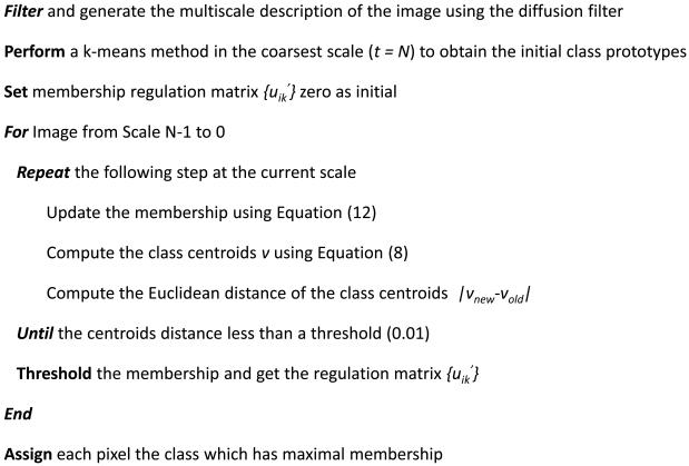
Starting from the original image (t=0), diffusion filtering progressively generates a series of images from the scale 0 to the scale N using Equation (13). At the coarsest image, the K-means method is applied to produce the initial hard classification of the image. Using the mean intensities of every class as the initial value of the next scale image classification, the algorithm iteratively computes the intensities of each class and the membership for every pixel according to Equations (8) and (12) until the characterized intensities of each class between two iterations are less than a threshold. Repeating this procedure to the image in the next scale, the classification stops as the procedure is done on the original image. The pseudo-code of the algorithm is expressed in Fig. 3.

Fig.3.

Pseudo-code of the multiscale fuzzy C-means classification (MsFCM) algorithm.

The weighting parameters for the scale information (β) and the neighboring information (α) generally depend on the noise level. For example, images with high noise need higher level spatial regularization from neighboring information and scale images. α and β are set as 0.85 in all our synthesized experiments. The conventional FCM is implemented by setting the constants α = β = 0 in the criteria function and by only performing the classification iteration in the original images. Similarly, the MFCM method is applied on the original images with α = 0.85 and β = 0 in the criteria function. These two methods are also initialized using the K-means method.

3. Image Classification Experiments and Validation

Our MsFCM classification method has been evaluated by synthetic images and McGill brain MR database (McConnel Brain Imaging Center, McGill University, Quebec, Canada) (Aubert-Broche et al., 2006; Kwan et al., 1996; Kwan et al., 1999). We also applied the method to classify real brain MR images and compared the results with manual segmentation. Meanwhile, MFCM and FCM methods were applied to these dataset in order to compare the performance of these three fuzzy classification methods.

3.1. Synthesized images for classification

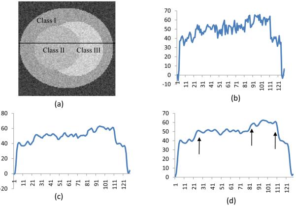
As shown n Fig.4a, the synthetic images represent a sphere-shape tumor with three tissue types (labeled as Class I, II, and III). In order to test the algorithm on images with poor contrast, we synthesized the images with different image quality. Contrast is defined as the relative intensity difference between one class and its surroundings.

$$\mathit{Contrast}(\%)=\frac{|I_o-I_b|}{I_b}\times 100$$ (15)

where I_b is the background intensity and I_o is the intensity of the object. We first give a preset intensity to the center sphere (Class II) and defined it as I_b. Intensities of Classes I and III are defined as I_o and are computed as I_o = I_b(1-contrast) for Class I and I_o = I_b(1+contrast) for Class III when a contrast is given.

Fig.4.

Anisotropic filter processing for a simulated noisy image. (a) is the original image labeled with three classes (Class I, II, III). The image is corrupted with noise. (b) is the signal profile along the labeled center line on Image (a). (c) and (d) are the signal profiles at Scale 5 and Scale 7 by diffusion filtering, respectively. The noise is removed and the line is smoothed. Furthermore, the edges are enhanced as shown by the arrows in (d).

After the image is created, 10% Gaussian noise with a mean of 0 is added to the images. The standard deviation of the added noise is 10% of the intensity of Class III. The SNR = 10. The image has a size of 128 × 128 pixels. For five different intensities (I_b = 30, 40, 50, 60, and 70) and six different contrasts = (60%, 50%, 40%, 30%, 20%, and 10%), a total of 30 images were synthesized to test the classification methods. For the three methods, MsFCM, MFCM, and FCM, 90 classification experiments were performed on the synthesized images. The overlap ratios of the classified results with the pre-defined truths are computed for each classification of each image.

3.2. MR brain phantoms for classification

We obtained the brain MR images from the McGill phantom brain database for comprehensive validation of the classification methods. The MR volume was constructed by subsampling and averaging a high-resolution (1-mm isotropic voxels), low-noise dataset consisting of 27 aligned scans from one individual in the stererotaxic space. The volume contains 181 × 217 × 181 voxels and covers the entire brain. A realistic brain phantom was then created from manual correction of an automatic classification of the MRI volume. Based on the realistic phantom, an MR simulator is provided to generate specified MR images. The MR tissue contrasts are produced by computing MR signal intensities from a mathematic simulation of the MR imaging physics (Kwan et al., 1996). The MR images also take the effects of various image acquisition parameters, partial volume averaging, noise, and intensity non-uniformity into account.

Using the MR simulator, we obtained T1-, T2-, and PD-weighted MR volumes with an isotropic voxel size of 1-mm and 20% intensity inhomogeneity at different noise percentages (3%, 5%, 7%, 9% and 15%). The intensity inhomogeneity was implemented by the MR volume multiplying a synthetic inhomogeneity field shape with the specified non-uniformity level. Prior to the classification, the extracranial tissues, such as skull, meninges, and blood vessels, had been removed manually so that the MR images for classification consisted of only three types of tissue, i.e. gray matter (GM), white matter (WM), and cerebrospinal fluid (CSF). The database also provides the ratio of each tissue type at each voxel. By assigning the voxel with the tissue type with a maximal ratio, the database also provides the ground truth for evaluation. We selected 2D transverse slices (Slices No.70, 98, 100, 102, and 130) for the classification evaluation. These MR data were applied to the three classification methods.

3.3. Real MR Images for classification

The classification method also was applied to real T1-weighted MR images of human brain. The MR images were acquired with a 4.0 Tesla MedSpec MRI scanner (Bruker BioSpin GmbH, Rheinstetten, Germany) on a Siemens Syngo platform (Siemens Medical Systems, Erlangen, Germany). T1-weighted magnetization-prepared rapid gradient-echo sequence (MPRAGE) (TR=2500 ms and TE=3.73 ms) was used for the image acquisition. The volume has 256 × 256 × 176 voxels covering the whole brain yielding 1.0 mm isotropic resolution. First, non-brain structure such as the skull was removed manually. Then, significant field inhomogeneity was corrected using a local entropy minimization and a bicubic spline model method (LEMS) (Salvado et al., 2006). Finally, manual segmentation of brain structures was performed to evaluate the classification. The MsFCM classification was performed with parameters α = β = 0.25.

3.4. Classification Evaluation

We used a variety of methods to evaluate the classification methods. First, we use overlap ratios between the classified results and the ground truth for classification evaluation. For synthesized images, the ground truth was known. For brain MR image data, the true tissue classification maps were obtained by assigning each pixel to the class to which the pixel most probably belongs. We used the Dice similarity measurement (DSM) (Cuadra, M. B. et al. 2005) to compute the overlap ratios. The DSM for each tissue type is computed as a relative index of the overlap between the classification result and the ground truth. It is as defined as:

$${\mathit{DSM}}^c=\frac{2{(A\cap B)}^c}{A^c+B^c}$$ (16)

Where A^c and B^c are the numbers of the pixels classified as Class c using our classification method and the ground truth, respectively; (A ∩ B)^cis the number of pixels classified as Class c in both results. This metric attains a value of one if the classified results are in full agreement with the ground truth and is zero when there is no agreement at all.

Secondly, the classification is evaluated by a confusion table, a table with two rows and two columns that reports the number of True Negatives (TN), False Positives (FP), False Negatives (FN), and True Positives (TP) for predictive analytics (Jaeschke et al., 2002). Similar to Cuadra, M. B. et al. (2005), the confusion table is computed as a matrix whose cells represent the ratio of the classified class on rows over the class of the ground truth on columns. Therefore, the diagonal entry represents the true positives (TP) for each class. The False Negative (FN) is defined as the percentage of the class of the ground truth mistakenly classified as the other classes. The False Positive (FP) of each class is computed as the percentage of the pixels incorrectly classified as the class over the pixels that do not belong to the class in the ground truth. The sensitivity of the classification method is calculated as TP/(TP+FN), and the specificity is defined as TN/(TN+FP).

4. Results

Fig. 4 demonstrates the effectiveness of the anisotropic filtering processing for the synthesized noisy image. In Fig. 4a, the synthesized image consists of three tissue types labeled as “Class I”, “Class II”, and “Class III”. Fig. 4b shows the intensity profile of the labeled sample line. Figs. 4c and 4d represent the intensity after the diffusion filtering processing at the scale levels 5 and 7, respectively. As the scale increases, the noise is smoothed within the each region, but the intensity difference at the edge has been enhanced so as to facilitate the classification (Fig. 4).

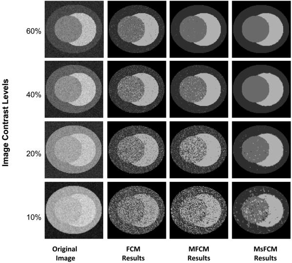
Fig. 5 illustrates the visual assessment of the classification results on synthesized tumor images and the comparison of the three methods. The synthesized images all have the same class distribution but different image contrasts labeled in each row. For the images with a high image contrast (60% and 40%), the three classification methods can successfully restore the class distribution. The MFCM and MsFCM methods have more homogeneous results than the FCM approach. However, our MsFCM achieved acceptable results even on images with very low contrast (10%) where the other two methods failed.

Fig.5.

Comparison of the classification results using the three methods for synthesized images. The first column contains the original images with the designed contrast level. The 2^nd, 3^rd and 4^th columns are the classification results using the FCM, MFCM, and MsFCM methods, respectively. The MsFCM method performs better than the other two methods for images with different contrast levels (10%-60%)

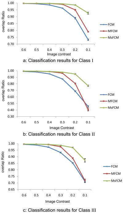
Fig. 6 shows the overlap ratios between the classification results and the ground truth for the three types of tissue (Class I, II, and III). The ratios decrease as the image contrast decreases. When the image contrast is higher than 40%, the three methods achieve accurate classification. When the contrast decreases, the performance of the FCM and MFCM decreases, but the MsFCM method can still achieve a high overlap ratio of more than 80%. The error bar represents the standard deviation of the DSM measurements computed from the classification of five images generated with a different mean intensity I_b. A standard deviation of less than 1% indicated consistent results for all three methods.

Fig.6.

Quantitative evaluation of the classification results for synthesized images with three classes I, II, and III. The Y axis is the overlap ratio between the ground truth and the classification results. The X-axis represents the contrast levels. Each data point represents 5 classification results from 5 images. Mean and standard deviation are plotted for each method. The MsFCM consistently works better than the other two methods for all of the three classes and contrast levels.

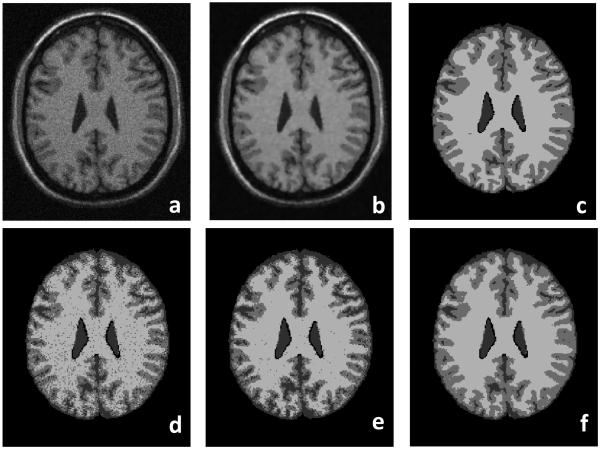
Fig. 7 demonstrates the classification results on T1-weighted brain MR images. Compared to the ground truth (Fig. 7c), our MsFCM method (Fig. 7f) performed better than the FCM (Fig. 7d) and the MFCM (Fig. 7e). The MsFCM method was applied to the images with different noise levels. Table 1 shows the overlap ratios for the different noise levels. The overlap ratios are greater than 90% for different noise levels indicating that our MsFCM method is not sensitive to noise.

Fig.7.

Classification results of brain MR images. The original MR image (a) is smoothed after the anisotropic filter processing (b). (c) is the ground truth of the classification. (d), (e), and (f) are the classification results using the FCM, MFCM, and MsFCM methods, respectively. Compared to the ground truth, the MsFCM performs better than the other two methods. The image was obtained from the McGill brain database with 9% noise and 20% intensity inhomogeneity.

Table 1.

The overlap ratios between the classification results and the ground truth for the brain data with respect to different noise levels for three types of tissue, i.e. cerebrospinal fluid (CSF), gray matter (GM), and white matter (WM).

	3%	5%	7%	9%
CSF	0.93 ± 0.02	0.93 ± 0.02	0.92 ± 0.03	0.90 ± 0.04
GM	0.94 ± 0.01	0.93 ± 0.01	0.91 ± 0.01	0.90 ± 0.01
WM	0.96 ± 0.01	0.96 ± 0.01	0.95 ± 0.02	0.94 ± 0.02

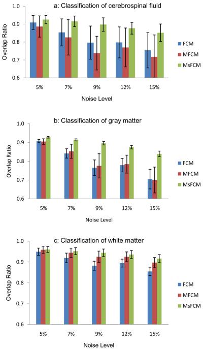
Fig. 8 shows the comparison results of the three methods for the images at different noise levels. Although the three methods have good results for images with low noises, MsFCM achieved overlap ratios of 88% ± 1% and 84% ± 1% for gray matter at the noise levels of 12% and 15%, respectively. However, for the same type tissue, the overlap ratios of the MFCM method were 78% ± 5% and 70% ± 6% for the same images at the noise levels of 12% and 15%, respectively. The overlap ratios of the FCM were 77 ± 3% and 70 ± 5%, respectively (Fig. 8b). Our MsFCM method consistently performed better than the other two methods for different tissues and for images at different noise levels.

Fig.8.

Overlap ratios of the classification results for the three methods, i.e. FCM, MFCM, and MsFCM. The images were obtained from the McGill brain database with 9% noise and 20% inhomogeneity. Each bar represent 5 classifications from 5 images, Mean and standard deviation are plotted. The MsFCM achieved higher overlap ratios compared to the other two methods.

Table 2 is the confusion table for the classification of the three methods. Although the false positive values of the MsFCM classification for CSF are higher than the other two methods, MsFCM achieved lower false negative and false positive values for gray matter and white matter. The FCM and MFCM methods incorrectly assign more pixels to Class CSF. As shown in Fig. 8, the overlap ratios of our MsFCM method are consistently higher than those of the other two methods for the MR images with different noise levels. The sensitivity and specificity of the MsFCM classification method are higher than those of the other two methods.

Table 2.

Evaluation of the classification results using the confusion tables. Tables from top to bottom represent the results for the MsFCM, MFCM, and FCM methods, respectively. On each table, the top row indicates the ground truth and the left column indicates the classified results. The value in each cell is the percentage against the ground truth. For example, the table at the top represents the results from the MsFCM method. For the column “CSF”, 96.77% pixels of the true CSF were correctly classified as Class “CSF”; 3.23% were incorrectly classified as Class “GM”; and none pixel was classified as Class “WM”. Thus, the false negative value is 3.23%. The images are T1-weighted MR images from McGill brain database with 9% noise and 20% field inhomogeneity.

MsFCM	Ground Truth
		CSF	GM	WM	FP
Classified Results	CSF	96.77±0.93	6.68±1.70	0.00±0.00	3.08±0.77
	GM	3.23±0.93	87.22±2.36	5.38±1.27	4.86±0.94
	WM	0.00±0.00	6.10±2.10	94.62±1.27	4.33±1.15
FN		3.23±0.93	12.78±2.36	5.38±1.27
MFCM	Ground Truth
		CSF	GM	WM	FP
Classified Results	CSF	99.30±0.61	22.39±11.16	0.03±0.06	9.99±4.30
	GM	0.69±0.61	68.48±7.77	6.34±1.53	5.07±1.28
	WM	0.01±0.02	9.13±4.86	93.63±1.56	6.44±3.01
FN		0.70±0.61	31.52±7.77	6.37±1.56
FCM	Ground Truth
		CSF	GM	WM	FP
Classified Results	CSF	97.62±1.21	16.75±7.01	0.03±0.04	7.52±2.60
	GM	2.37±1.21	72.47±4.23	13.19±2.52	10.76±2.29
	WM	0.01±0.02	10.78±4.70	86.78±2.55	7.64±2.85
FN		2.38±1.21	27.53±4.23	13.22±2.55

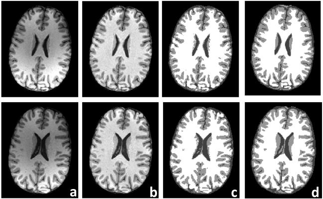
Classification results on real MR brain data were showed on Fig. 9. Significant intensity inhomogeneity was observed in the MR images (Fig. 9a), which was corrected and shown in Fig. 9b. MsFCM image classification (Fig .9c) was performed on different slices and the overlap ratios were 85% ± 3% for CSF, 82% ± 5% for gray matter, and 88% ± 4% for white matter (Fig. 9d).

Fig.9.

Classification of real brain MR volume. Results of two slices are showed in rows. The first column (a) is the original MR images. The second column (b) is the images after intensity inhomogeneity correction. The third column (c) is the MsFCM classification results on the corrected images where three gray levels represent the CSF, gray matter, and white matter, respectively. The last column (d) is the manual segmentations for evaluating the MsFCM classification.

5. Discussion and Conclusions

We developed and evaluated a multiscale fuzzy c-means classification method for MR images. We used an anisotropic filter to effectively attenuate the noise within the images but to preserve the edges between different tissue types. A scale space was generated by anisotropic filtering, and the general structure information was kept in the images at a coarser scale. The classification was advanced along the scale space to include local information in the fine-level images. The result from a coarser scale provides the initial parameter for the classification in the next scale. Meanwhile, the pixels with a high probability of belonging to one class in the coarse scale will belong to the same class in the next level. Therefore, these pixels in the coarser images are considered as pixels with a known class and are used as the training data to constrain the classification in the next scale. In this way, we obtain accurate classifications step-by-step and avoid being trapped into local minima. Furthermore, we also include a regulation term that constrains the pixel so that it can be influenced by its immediate neighborhoods. Using the multiscale classification, higher spatial information is also included in the MsFCM method. This approach can achieve a piecewise-homogeneous solution. Our method was evaluated using synthesized images, a brain MR database, and our real brain MR data. The classification method is accurate and robust for noisy images with low contrast.

Our method was compared with FCM and MFCM and achieved consistent better results. We also compared our method with Gaussian Markov random field classification on brain phantom data with 15% noise and 20% inhomogeneity. MsFCM got a marginal improvement with overlap ratios of 85% ± 5% for CSF, 84% ± 1% for gray matter, and 92% ± 2% for white matter while the overlap ratios from the Gaussian Markov random field classification were 83% ± 2% for CSF, 81% ± 3% for gray matter, and 88% ± 2% for white matter. This improvement is marginal because Gaussian function is a good model for intensity distribution of normal brain structure. We expected better results from MsFCM for those images such as tumor images that deviate from a Gaussian distribution.

The multiscale scheme improves not only the speed of the classification but also the robustness. The centroids of the initial classes from the coarser image improve the convergence of the classification algorithm. A pixel with a high probability of belonging to one class in the coarse image is expected to belong to the same class in the next fine image. The threshold κ is used to select these voxels at the coarse level and thus to constrain the classification in the next level. A smaller threshold means more reliable classification in the coarse image. This threshold depends on noise levels and preprocessing such as diffusion filtering. A smaller threshold is expected for images with better image quality. At the coarse level, the threshold κ in Equation (6) was set to 0.85 for our MR images. Our simulation data demonstrated that the classification method was not sensitive to the threshold when it is between 0.8 and 0.9. However, the threshold value may need to be adjusted accordingly when this method is applied to other images with a different noise level.

The algorithm is implemented in Matlab 7.1 (MathWorks, Natick, MA) with a desk computer (3GHz Pentium IV processer and 3G bytes RAM). Normally, the classification on one scale converges within 3~4 iterations. The classification takes approximately three minutes that can be significantly reduced if C++ and a high-performance workstation are used for the computation. The method can be applied to 3D volume data where 26 neighboring pixels are considered. This could include more spatial regularization and lead to a better result. However, a fast 3D diffusion filtering algorithm is required.

If there is significant field inhomogeneity on MR images, it could possibly affect the classification results. Fortunately, various inhomogeneity correction methods can be used as a pre-processing step before classification (Liew et al., 2003; Salvado et al., 2006). We applied inhomogeneity correction on real brain MR data and achieved satisfied results. As our classification method did not assume a Gaussian distribution of tissue intensity, it could be used on other image data such as histologic images for tissue classification and quantification. The automatic classification method can provide a useful, quantification tool in neuroimaging and other applications.

References

- Ahmed MN, Yamany SM, Mohamed N, Farag AA, Moriarty T. A modified fuzzy C-means algorithm for bias field estimation and segmentation of MRI data. IEEE Trans Med Imaging. 2002;21(3):193–199. doi: 10.1109/42.996338. [DOI] [PubMed] [Google Scholar]
- Aubert-Broche B, Evans AC, Collins L. A new improved version of the realistic digital brain phantom. Neuroimage. 2006;32(1):138–145. doi: 10.1016/j.neuroimage.2006.03.052. [DOI] [PubMed] [Google Scholar]
- Bezdek J. a convergence theorem for the fuzzy ISODATA clustering algorithms. IEEE Trans Pattern Anal.Machine Intell. PAMI(2) 1980:1–8. doi: 10.1109/tpami.1980.4766964. [DOI] [PubMed] [Google Scholar]
- Canny J. A computational approach to edge detection. IEEE Trans Pattern Anal.Machine Intell. 1986;8:679–698. [PubMed] [Google Scholar]
- Carano RA, Ross AL, Ross J, Williams SP, Koeppen H, Schwall RH, Van Bruggen N. Quantification of tumor tissue populations by multispectral analysis. Magn Reson Med. 2004;51(3):542–551. doi: 10.1002/mrm.10731. [DOI] [PubMed] [Google Scholar]
- Chen S, Zhang D. Robust image segmentation using FCM with spatial constraints based on new kernel-induced distance measure. IEEE Trans Syst Man Cybern B Cybern. 2004;34(4):1907–1916. doi: 10.1109/tsmcb.2004.831165. [DOI] [PubMed] [Google Scholar]
- Choi HS, Haynor DR, Kim Y. Partial volume tissue classification of multichannel magneticresonance images-a mixel model. IEEE Trans Med Imaging. 1991;10(3):395–407. doi: 10.1109/42.97590. [DOI] [PubMed] [Google Scholar]
- Cocosco CA, Zijdenbos AP, Evans AC. A fully automatic and robust brain MRI tissue classification method. Med Image Anal. 2003;7(4):513–527. doi: 10.1016/s1361-8415(03)00037-9. [DOI] [PubMed] [Google Scholar]
- Cuadra MB, Cammoun L, Butz T, Cuisenaire O, Thiran JP. Comparison and validation of tissue modelization and statistical classification methods in T1-weighted MR brain images. IEEE Trans Med Imaging. 2005;24(12):1548–1565. doi: 10.1109/TMI.2005.857652. [DOI] [PubMed] [Google Scholar]
- Held K, Rota KE, Krause BJ, Wells WM, III, Kikinis R, Muller-Gartner HW. Markov random field segmentation of brain MR images. IEEE Trans Med Imaging. 1997;16(6):878–886. doi: 10.1109/42.650883. [DOI] [PubMed] [Google Scholar]
- Jacobs MA, Zhang ZG, Knight RA, Soltanian-Zadeh H, Goussev AV, Peck DJ, Chopp M. A model for multiparametric mri tissue characterization in experimental cerebral ischemia with histological validation in rat: part 1. Stroke. 2001;32(4):943–949. doi: 10.1161/01.str.32.4.943. [DOI] [PubMed] [Google Scholar]
- Jaeschke R, Guyatt G, Lijmer J. Diagnostic tests. In: G Guyatt, D Rennie., editors. Users' Guides to the Medical Literature. AMA Press; Chicago: 2002. [Google Scholar]
- James M. Classification Algorithms. John Wiley; New York: 1985. [Google Scholar]
- Kwan RK, Evans AC, Pike GB. Lecture Notes in Computer Science. Vol. 1131. Springer-Verlag; 1996. An Extensible MRI Simulator for Post-Processing Evaluation, Visualization in Biomedical Computing (VBC'96) pp. 135–140. [Google Scholar]
- Kwan RK, Evans AC, Pike GB. MRI simulation-based evaluation of image-processing and classification methods. IEEE Trans Med Imaging. 1999;18(11):1085–1097. doi: 10.1109/42.816072. [DOI] [PubMed] [Google Scholar]
- Li L, Jiang Q, Ding G, Zhang L, Zhang ZG, Ewing JR, Knight RA, Kapke A, Soltanian-Zadeh H, Chopp M. Map-ISODATA demarcates regional response to combination rt-PA and 7E3 F(ab')2 treatment of embolic stroke in the rat. J Magn Reson Imaging. 2005;21(6):726–734. doi: 10.1002/jmri.20318. [DOI] [PubMed] [Google Scholar]
- Liew AW, Yan H. An adaptive spatial fuzzy clustering algorithm for 3-D MR image segmentation. IEEE Trans Med Imaging. 2003;22(9):1063–1075. doi: 10.1109/TMI.2003.816956. [DOI] [PubMed] [Google Scholar]
- Lu D, Weng Q. A survey of image classification methods and techniques for improving classification performance. International Journal of Remote Sensing. 2007;28(5):823–870. [Google Scholar]
- Marroquin JL, Vemuri BC, Botello S, Calderon F, Fernandez-Bouzas A. An accurate and efficient bayesian method for automatic segmentation of brain MRI. IEEE Trans Med Imaging. 2002;21(8):934–945. doi: 10.1109/TMI.2002.803119. [DOI] [PubMed] [Google Scholar]
- Noordam JC, Van den broek WHAM, Buydens LMC. Geometrically guidedd fuzzy C-means clustering for multivariate image segmentation. Proc.Int.Conf.on Pattern Recognition. 2000;1:462–465. [Google Scholar]
- Perona P, Malik J. Scale-space and edge detections using anistropic diffusion. IEEE Trans Pattern Anal.Machine Intell. 1990;12(7):629–639. [Google Scholar]
- Pham DL, Prince JL. Adaptive fuzzy segmentation of magnetic resonance images. IEEE Trans Med Imaging. 1999;18(9):737–752. doi: 10.1109/42.802752. [DOI] [PubMed] [Google Scholar]
- Salvado O, Hillenbrand C, Zhang S, Wilson DL. Method to correct intensity inhomogeneity in MR images for atherosclerosis characterization. 2006;25(5):539–552. doi: 10.1109/TMI.2006.871418. [DOI] [PubMed] [Google Scholar]
- Tolias YA, Panas SM. On applying spatial constraints in fuzzy image clustering using a fuzzy rule-based system. IEEE Signal Processing Letters. 1998;5:245–247. [Google Scholar]
- Van Leemput K, Maes F, Vandermeulen D, Suetens P. Automated model-based tissue classification of MR images of the brain. IEEE Trans Med Imaging. 1999;18(10):897–908. doi: 10.1109/42.811270. [DOI] [PubMed] [Google Scholar]
- Young TY, Fu K-S, editors. Handbook of Pattern Recognition and Image Processing. Academic Press; 1986. [Google Scholar]
- Zhang Y, Brady M, Smith S. Segmentation of brain MR images through a hidden Markov random field model and the expectation-maximization algorithm. IEEE Trans Med Imaging. 2001;20(1):45–57. doi: 10.1109/42.906424. [DOI] [PubMed] [Google Scholar]