

Abstract
A confound for functional magnetic resonance imaging (fMRI), especially for auditory studies, is the presence of imaging acoustic noise generated mainly as a byproduct of rapid gradient switching during volume acquisition and to a lesser extent, the radio-frequency transmit. This work utilized a novel pulse sequence to present actual imaging acoustic noise for characterization of the induced hemodynamic responses and assessment of linearity in the primary auditory cortex with respect to noise duration. Results show that responses to brief duration (46ms) imaging acoustic noise is highly nonlinear while responses to longer duration (>1s) imaging acoustic noise becomes approximately linear, with the right primary auditory cortex exhibiting a higher degree of nonlinearity than the left for the investigated noise durations. This study also assessed the spatial extent of activation induced by imaging acoustic noise, showing that the use of modeled responses (specific to imaging acoustic noise) as the reference waveform revealed additional activations in the auditory cortex not observed with a canonical gamma variate reference waveform, suggesting an improvement in detection sensitivity for imaging acoustic noise-induced activity. Longer duration (1.5s) imaging acoustic noise was observed to induce activity that expanded outwards from Heschl’s gyrus to cover the superior temporal gyrus as well as parts of the middle temporal gyrus and insula, potentially affecting higher level acoustic processing.
Keywords: imaging acoustic noise, functional MRI, hemodynamic response, linear systems
INTRODUCTION
The presence of acoustic noise in functional magnetic resonance imaging (fMRI) is a confounding factor that has long been a concern for the experimental community, especially for those conducting fMRI studies requiring accurate perception of complex auditory stimuli. This acoustic noise (hereafter referred to as imaging acoustic noise) is a byproduct of the echo planar imaging acquisition technique typically employed for fMRI, sometimes achieving intensity levels at or above 110 decibels sound pressure level (dB SPL) (Ravicz et al., 2000). Imaging acoustic noise not only alters the sensory perception of the desired auditory stimuli (Hall et al., 2009), but also has been shown to produce blood oxygenation level-dependent (BOLD) responses in the auditory cortex potentially interfering with responses to desired auditory stimuli (Bandettini et al., 1998; Talavage et al., 1999; Novitski et al., 2001; Moelker et al., 2003; Talavage and Edmister, 2004).
Characterization of the hemodynamic response induced by imaging acoustic noise and subsequent assessment of linearity is crucial for the development of effective compensation methods that may account for the effects of imaging acoustic noise in auditory fMRI. Tamer et al. (2009) observed that the hemodynamic response induced by an “elemental unit” of imaging acoustic noise (i.e. from acquisition of a single slice) is concomitant in amplitude to that induced by a typical acoustic stimulus. For a brief duration acoustic stimulus, such as an elemental unit of imaging acoustic noise, the hemodynamic response is expected to be highly nonlinear. Soltysik et al. (2004) observed nonlinearity in the primary auditory cortex to trains of 125ms pure tone bursts (spaced 125ms apart) lasting up to 10s in duration, but for longer duration stimuli, responses became approximately linear. Similarly, Robson et al. (1998) observed nonlinear behavior in the primary auditory cortex to trains of 100ms tone bursts (spaced 100ms apart) lasting less than 6s in duration. As imaging acoustic noise consists of brief 46ms bursts of spectrally complex “pings,” the induced hemodynamic responses can be expected to differ somewhat from the responses obtained in the aforementioned studies, although the general trend is expected to be similar.
Mitigation of the effects of imaging acoustic noise has been previously sought through modifications of scanner hardware (Ravicz et al., 2000; Edelstein et al., 2002; Edelstein et al., 2005) and through the addition of passive attenuation measures in the experimental setup (Ravicz et al., 2000), the simplest of which involves the use of earmuff and/or eartips to achieve passive attenuation of up to approximately 45 dB. Though passive attenuation reduces the intensity of imaging acoustic noise, the subsisting imaging acoustic noise remains clearly audible to the subject. This subsisting imaging acoustic noise is transmitted by both air conduction, via the ear canal, and bone conduction, via the direct contact between skeletal (including cranial) bones and the vibrating coil base and patient bed assembly (Ravicz et al., 2001). Alleviation of the effects of imaging acoustic noise has also been sought through experimental efforts such as the usage of clustered volume acquisition (Edmister et al., 1999) to allow presentation of auditory stimuli in the quiescent period between volume acquisitions, mitigating masking of the desired stimuli by imaging acoustic noise. Clustered volume acquisitions are commonly employed with a longer repetition time to further reduce the interaction between noise- and stimulus-induced responses, but come at the cost of decreased statistical power, necessitating either recruitment of a larger subject pool or longer experiments. While successful in achieving their primary goals, these efforts cannot achieve optimality (i.e., no noise perception), and the noise remains a critical consideration in auditory fMRI.
Characterization of the BOLD response to imaging acoustic noise and subsequent modeling of the interaction between the response to this noise and the response to the desired stimuli may be the best procedure for improving auditory fMRI experiments. Previous studies utilized recorded scanner background noise (Gaab et al., 2007; Hall et al., 2000), which does not take into account physical stimulation through bone conduction and vibration of the patient bed assembly (Ravicz et al., 2001; Hiltunen et al., 2004; Tomasi et al., 2004). This work utilizes radio-frequency disabled volume gradient sequences in between actual clustered volume acquisitions (Edmister et al., 1999) to generate real imaging acoustic noise without perturbing longitudinal magnetization. The objectives of this work are to assess the linearity of the responses induced by imaging acoustic noise and to examine the changes in the spatial extent of brain activation with respect to the duration/quantity of imaging acoustic noise. Assessment of the linearity of imaging acoustic noise-induced responses will enable prediction of distortions to the shape of the desired response while characterization of the extent of spatial activation arising from imaging acoustic noise will enable prior identification of those areas most likely to be negatively affected by the presence of imaging acoustic noise. In addition, knowledge gained from these efforts will likely provide further insight into cortical behavior and function.
MATERIALS AND METHODS
Paradigm
Radio-frequency (RF) disabled volume gradient sequences, henceforth referred to as dummy volumes, were applied at variable post-offset sample times between actual volume acquisitions. These dummy volumes were generated using a normal blipped EPI slice acquisition with a zero-amplitude RF pulse, generating imaging acoustic noise (i.e. a “ping” sound for each slice of the dummy volume) without perturbing longitudinal magnetization. The imaging acoustic noise intensity on the General Electric 1.5 T Signa CVi used in this study is approximately 97 dB SPL.
Three experiments were conducted, in each of which a dummy volume, comprising a 1-, 10-, or 15-slice RF-disabled gradient sequence, was effected to generate 1-, 10-, and 15-ping imaging acoustic noise, respectively. The gradient sequence was grouped as per a clustered volume acquisition (CVA) (Edmister et al., 1999) and generated in the quiescent period between actual CVAs, occurring at a fixed TR. The 1-slice RF-disabled gradient sequence generated a single ping imaging acoustic noise 46 ms in duration that occurs approximately 20 ms into a 100 ms duration pulse sequence. Note that all analysis in this work is performed with respect to the onset of the pulse sequence. The 10-ping (1 s overall duration) and 15-ping (1.5 s overall duration) stimuli consist of trains of perceptually distinct 46 ms pings occurring at a rate of approximately 10 per second. The generated ping stimuli are spectrally diverse, containing many distinct peaks in the audible frequency range (Tamer et al., 2009). For all three cases, the delay between a dummy volume and the subsequent actual volume acquisition was varied over a set of post-offset (relative to the dummy volume) sampling times (Table 1) using a stroboscopic paradigm (Belin et al., 1999), including a null condition in which no dummy volume was generated. Variation of the temporal position of the dummy volume between actual image acquisitions enables the measurement of the hemodynamic response induced by pure imaging acoustic noise produced by the dummy volume, as depicted in Figure 1. Twelve trials of each post-offset sample time and the null condition were acquired for each experiment. The long TR values (26 s for 1-ping; 33 s for 10- and 15-ping experiments) were used to permit the hemodynamic response induced by the previous volume acquisition to approach baseline prior to the presentation of the dummy volume.
Table 1.
Post-offset sample times for 1-, 10-, and 15-slice dummy volume experiments. Note that times are measured relative to the offset of the dummy volume. A null condition was also acquired in which no dummy volume was presented.
| Dummy Volume | TR (s) | # Sample Times | Variable Post-Offset Sample Times (s) |
|---|---|---|---|
| 1-slice | 29 | 9 | 1.5, 3, 3.5, 4, 5, 6.5, 7.5, 8.5, 12.5 |
| 10-slice | 33 | 7 | 2, 2.5, 3, 4, 5.5, 7.5, 11.5 |
| 15-slice | 33 | 14 | 1.5, 2, 2.5, 3, 3.5, 4, 5, 7, 9, 10, 11, 12.5, 14, 15 |
Figure 1.
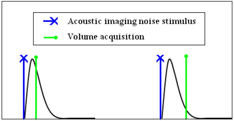
Illustration of stroboscopic experimental paradigm (e.g., Belin et al., 1999) showing volume acquisitions occurring with a fixed repetition time sampling the hemodynamic response induced by imaging acoustic noise at variable post-offset sample times.
During the scanning session, subjects wore earmuffs with custom eartips, achieving overall attenuation of approximately 42 dB. The eartips were connected to a pneumatic sound delivery system via inserted plastic tubing to mimic the setup of a typical auditory fMRI experiment, but no acoustic stimulus was delivered through the pneumatic system. During the functional runs, subjects viewed a self-chosen movie that was projected onto a screen and viewed through a mirror without subtitles or sound. The use of a subject-selected movie (typically chosen to be an action movie with minimal dialog) served to maintain subject interest in and attention to the presented visual stimulus, enabling the assessment of brain response to the imaging acoustic noise as the subjects listened in a passive manner, mimicking a typical experiment in which the imaging acoustic noise is not the intended target of attention.
Subjects
40 adult subjects (20 male, 20 female) were imaged on a General Electric 1.5 T Signa CVi (InnerVision Advanced Medical Imaging; Lafayette, IN). All subjects reported normal hearing with no history of hearing impairment, and gave written informed consent prior to participation in the study. A group of 20 subjects underwent one scanning session in which a 15-ping train was used as the auditory stimulus, and a second group of 20 subjects participated in a single session in which responses to trains of 1- and 10-ping imaging acoustic noise were measured. All subjects were instructed to lie still and watch the movie during the functional runs.
Imaging Protocol
Each imaging session consisted of four data acquisition segments: (1) a high-resolution anatomical reference dataset using a standard birdcage head coil (124 slices; in-plane resolution = 0.9375 mm × 0.9375 mm), (2) a sagittal localizer to identify desired imaging volume, (3) high-resolution (in-plane = 0.9375 mm × 0.9375 mm) images of the desired imaging volume, and (4) functional scans (TE = 40 ms, flip angle = 90°, FOV = 24 cm, in-plane resolution = 3.75 mm × 3.75 mm). The desired imaging volume consisted of fifteen 3.8 mm thick axial slices (thickness chosen to obtain isotropic voxels) centered on Heschl’s gyrus to ensure acquisition of the whole auditory cortex. With the exception of the anatomical reference dataset, all acquisition segments were acquired using bilateral auditory surface coils designed to maximize contrast to noise ratio in the auditory cortex region.
Correction of Dummy Volume Induced Artifact
The usage of dummy volumes to generate imaging acoustic noise induced artifactual signal fluctuations that varied with respect to the temporal position of the dummy volume in between actual volume acquisitions. Hu et al. (2009) characterized this artifact as exhibiting exponentially decaying and oscillatory behavior, caused by eddy currents and gradient coil heating induced by the dummy volume in between actual CVAs. Dummy volumes of 1.5 s in duration produced large (~0.3% peak signal change) artifactual fluctuations, therefore data from the 15-slice experiment were corrected using a modified projection algorithm as per Hu et al. (2009), prior to preprocessing.
Preprocessing
Image analysis was performed using AFNI (Cox et al., 1996). For each session, all functional images were realigned to the third image of the first run to correct for subject motion, and any runs exhibiting translational motion above 1.5 mm in either x, y, or z directions were discarded. The realigned functional runs were then registered to the subject’s reference anatomical dataset to allow identification of structures of interest.
ROI Selection
To estimate the HDR induced by imaging acoustic noise, regions of interest (ROIs) were constructed for each subject in the left and right hemispheres, using the acquired 3D-SPGR anatomical dataset as reference. Note that ROIs were constructed using each subject’s untransformed (i.e. prior to Talairach conversion) anatomical volumes and the corresponding untransformed EPI images to generate precise definition of ROIs on an individual subject basis. The ROIs were chosen to be the left and right primary auditory cortices consisting of both white and gray matter, located in the postero-medial two-thirds of the first (most anterior) Heschl’s gyrus, most consistent with the area consisting of medial (KAm) and lateral (KAlt) koniocortex, as defined by Galaburda and Sanides (1980). The lateral boundary of Heschl’s gyrus was chosen to be the border with the anterior temporal gyrus, and the medial boundary was defined as the line connecting the medial end of the first transverse sulcus to the medial end of the anterior Heschl’s gyrus. The x-coordinates of the medial and lateral boundaries of Heschl’s were defined and recorded on an individual subject basis over all slices that included Heschl’s gyri, and the voxels within the medial two-thirds (Figure 2) of this range comprised the regions of interest in the left and right hemispheres. The remaining antero-lateral one-third of Heschl’s gyrus, although primary-like, is typically not considered part of the primary auditory cortex, and is excluded from the ROI. For this study, the average selected ROI size±standard deviation over all subjects is 1045±217 mm3 for the left primary auditory cortex and 791±229 mm3 for the right primary auditory cortex.
Figure 2.
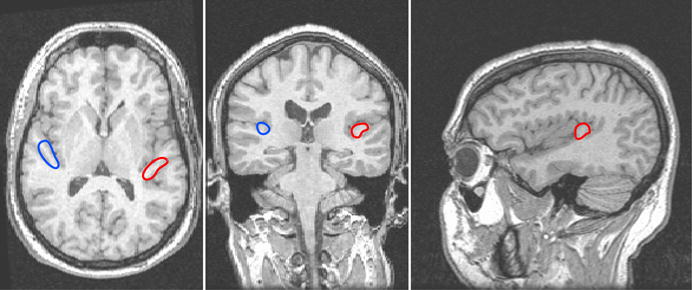
Illustration of manually-selected primary auditory cortex ROI from a subject’s anatomical images. The left ROI is shown in red and the right ROI in blue.
Percent Signal Change Calculation
Hemodynamic responses for the ROIs were estimated by calculating the percent signal change induced by the stimulus at each offset sample time with respect to the null stimulus for each voxel inside the ROIs. Group-averaged HDR estimates were obtained in the left and right auditory cortices by performing a weighted mean (depending on the number of runs remaining after screening for motion) across voxels, runs, and subjects.
Fitting HDRs to Double Gamma Variate Model
The group-average HDR estimates for the 1-, 10-, and 15-ping imaging acoustic noise were fitted to the double gamma variate model (Glover et al., 1999), defined in Eq. 1.
| (1) |
The double gamma variate model, based on the gamma variate model of Boynton et al. (1996), consists of two gamma variate functions, one to model the rise to peak and another to model the undershoot. This model contains parameters to model the amplitude of the peak and undershoot (A1, A2), the onset delay of the peak and undershoot following stimulation (δ1, δ2), and the duration of the response (τ1, τ2). Nonlinear regression was performed using MATLAB (The Mathworks Inc., Natick, MA) to fit the group-averaged HDR estimates induced by the 1-, 10-, and 15-ping imaging acoustic noise to the model.
Assessment of Nonlinear Properties
The property of superposition for linear systems, represented in Eq. 2, is used to assess if hemodynamic responses in the primary auditory cortex induced by imaging acoustic noise exhibited nonlinear characteristics.
| (2) |
In Eq. 2, T[x(t)] is the response system T exhibits from input waveform x(t) with a and b representing scaling constants. The system is assumed to be time-invariant – if an input to the system is shifted by a given time delay, then the output of the system is shifted by the same time delay. Vazquez et al. (1998) used the principle of superposition and the assumption of time-invariance to assess the linearity of hemodynamic responses in the primary visual cortex (V1) by adding time-delayed responses induced by shorter duration stimuli to predict responses induced by longer duration stimuli under the assumption of linearity. The predicted response was compared to the actual response of the longer duration stimuli in terms of peak amplitude to assess the degree of nonlinearity (Vazquez et al., 1998).
For this study, the fitted responses for the 1-, 10-, and 15-ping imaging acoustic noise were used in the linearity analysis. This choice was made based upon the coarse sampling of the estimated responses, which additionally are likely to contain residual noise. To assess whether the 1-ping response is predictive of the 10-ping response, ten 1-ping fitted responses were successively time delayed by 0.1 s and added to form the 10-ping linear system response. The 10-ping linear system response was then compared to the 10-ping fitted response in terms of peak amplitude and coefficient of determination to assess the degree of nonlinearity for brief duration imaging acoustic noise. Similarly, to assess whether the 1-ping response is predictive of the 15-ping response, fifteen 1-ping responses were delayed and added to form the 15-ping linear systems response. In order to determine whether the 10-ping response is predictive of the 15-ping response, the comparison procedure was altered as the 15-ping stimuli is not an integer multiple of the shorter 10-ping stimuli. 30-ping linear system responses were formed from (a) three time-delayed and superimposed 10-ping responses and (b) two time-delayed and superimposed 15-ping responses; the two different 30-ping linear system responses generated using (a) and (b) were then compared to assess the degree of nonlinearity for the longer duration imaging acoustic noise.
Statistical Analysis
In assessing the brain regions adversely affected by imaging acoustic noise of varying duration, this work sought to improve the detection of imaging acoustic noise-induced activations through the use of fitted responses specific to imaging acoustic noise as the reference waveform input to linear regression. The statistical maps generated with the fitted responses as the reference waveforms were compared to those generated with a canonical gamma variate reference waveform in order to assess whether using the fitted waveforms offered an improvement over using the canonical waveform for linear regression. The statistical analysis procedure is presented in detail as follows.
All preprocessed datasets were spatially transformed into Talairach space using the single subject, skull-stripped TT_N27 AFNI template. The normalized images were then spatially smoothed with a Gaussian kernel of 4 mm full-width-at-half-maximum (FWHM). For linear regression (3dDeconvolve), the fitted responses were first used as the reference waveforms to probe for acoustic imaging induced-activations. The reference waveforms were generated on an individual subject basis and evaluated using a k-cross validation scheme (Kearns et al., 1996). In the k-cross validation scheme, the reference waveforms for each subject were the fitted responses to 1-, 10-, and 15-ping imaging acoustic noise generated using the functional runs acquired from the other nineteen subjects, avoiding over-fitting associated with the use of the target data in generation of the reference waveform. Following linear regression, a mask comprising 4573 voxels was generated using 3dAutomask in AFNI, eliminating regions in the datasets where signal level was too low for valid statistical assessment. Then, one factor (multiple subject) random effects analysis was performed to generate t-statistic maps for the 1-, 10-, and 15-ping experiments. Correction for multiple comparisons was effected via the Bonferroni method and statistical maps were displayed at an alpha-level of 0.05 (pBonferroni<0.05).
To assess whether the use of fitted responses as the reference waveform was advantageous over the use of a canonical reference waveform, the analysis procedure described above was then repeated using the gamma variate function provided by AFNI as the canonical reference waveform for linear regression. The gamma variate function is show in Eq. 3; default parameters b = 8.6 and c = 0.547 were used.
| (3) |
Analysis of Extent of Activation
To quantify the extent of activation induced by the 1-, 10-, and 15-ping imaging acoustic noise, an auditory cortex mask with 183 voxels (11712 mm3) was defined in the left hemisphere of the TT_N27 AFNI brain template, consisting of Heschl’s gyrus and the superior temporal gyrus. The superior temporal gyrus was defined as the region between the sylvian fissure and the superior temporal sulcus, with the posterior boundary being the intersection of the horizontal ramus of the sylvian fissure and ascending ramus of the superior temporal sulcus as in Taylor et al. (2005). Heschl’s gyrus was selected as defined previously. A similar auditory cortex mask encompassing 179 voxels (11456 mm3) was defined in the right hemisphere. These masks were chosen to include primary and secondary auditory cortices in order to tabulate the number of auditory activations induced by imaging acoustic noise of varying duration. Using the defined left and right masks, the number of active voxels was tallied at pBonferroni < 0.05 for the 1-, 10-, and 15-ping experiments.
Assessment of Goodness-of-Fit
The coefficient of determination, R2, is a common metric used – in mathematics to assess the goodness of fit. R2 is defined as one minus the ratio between the sum of squared errors and the regression sum of squares, and is bounded between 0 and 1 with 1 denoting a perfect fit. The coefficient of determination was calculated to assess how well the double gamma variate function modeled the group-averaged estimated hemodynamic responses as well as to compare the linear system responses and the fitted responses in assessing the degree of nonlinearity. This metric enables the comparison of two complete time courses for the purposes of this study, whereas statistical tests of significance such as the t-test can only be used to compare values at each post-offset sample time of two time courses. It should be noted that the disadvantage of the coefficient of determination is the lack of an associated p-value denoting whether the waveforms are significantly different. While R2 does not have an associated p-value, it can be used to assess whether one fit is better than another by comparing the values of the coefficient of determination.
RESULTS
Imaging Acoustic Noise-Induced HDRs and Fitting
Figure 3 shows the group-averaged estimated hemodynamic response samples in green for the left and right auditory cortex ROIs induced by 1-, 10-, and 15-ping imaging acoustic noise; the x-axis represents the post-onset sample time in seconds. The double gamma variate fits are overlaid in red in Figure 3, with fitting parameters tabulated in Table 2. As the imaging acoustic noise duration increased, the induced responses also increased in amplitude in the left and right ROIs. Whereas the 1-ping imaging acoustic noise induced responses returned to baseline (defined as the value of the null acquisition) by approximately 13s, the 15-ping induced response returned to baseline by approximately 15s. To assess how well the double gamma variate function modeled the estimated responses, the coefficients of determination were calculated and displayed in Figure 3. For the left ROI, the calculated coefficients of determination were R21-ping=0.80, R210-ping=0.97, and R215-ping=0.99; for the right ROI the calculated coefficients of determination were R21-ping=0.61, R210-ping=0.96, and R215-ping=0.93. These values indicate that the fits were better for the longer duration 10- and 15-ping imaging acoustic noise-induced hemodynamic responses, especially for the left ROI which exhibited less variance in the estimated hemodynamic responses. For the 10- and 15-ping fitted responses, R2 ≥ 0.93 represent excellent fits.
Figure 3.

Modeled hemodynamic responses, fit using a double-gamma variate function (red lines; model has six parameters), overlaid with group-averaged estimated hemodynamic response samples (green points; mean ± one standard error) for (a) left and (b) right regions of interest for (top) 1-ping, (middle) 10-ping, and (bottom)15-ping imaging acoustic noise. The coefficient of determination (R2) is a measure of the goodness-of-fit between the double gamma variate model and the estimated hemodynamic response samples.
Table 2.
Fitted parameters of the double gamma variate model for the group-averaged estimated 1-, 10-, and 15-ping hemodynamic responses, for left and right ROIs (see Figure 3).
| Left ROI | Right ROI | |||||
|---|---|---|---|---|---|---|
| 1-ping | 10-ping | 15-ping | 1-ping | 10-ping | 15-ping | |
| A1 | 0.45 | 2.05 | 1.36 | 0.59 | 1.77 | 1.12 |
| δ1 | 1.4 | 2.1 | 1.7 | 1.0 | 2.3 | 1.5 |
| τ1 | 1.0 | 1.9 | 1.4 | 1.5 | 1.9 | 1.6 |
| A2 | 0.21 | 2.06 | 1.02 | 0.17 | 1.86 | 0.73 |
| δ2 | 4.4 | 3.0 | 5.4 | 2.0 | 3.0 | 6.0 |
| τ2 | 1.46 | 1.9 | 1.3 | 2.5 | 1.9 | 1.2 |
Assessment of Nonlinear Properties
To assess the degree of nonlinearity exhibited by the primary auditory cortex, responses to the longer duration ping trains were modeled using linear system theory as superposition of time-delayed responses to shorter duration imaging acoustic noise, and subsequently compared to the actual fitted responses in terms of peak amplitude. Figure 4 depicts the linear system responses overlaid with the fitted responses for the left and right primary auditory cortex.
Figure 4.

Linearity assessment of hemodynamic response in the left and right primary auditory cortices to imaging acoustic noise through comparison of modeled hemodynamic responses. (a) 10-ping linear system response (HDR10_1) formed from superposition of 10 successively time-delayed 1-ping responses, overlaid with the fitted 10-ping response (HDR10); (b) 15-ping linear system response (HDR15_1) overlaid with fitted 15-ping response(HDR15); (c) 30-ping linear system response formed from superposition of two 15-ping responses (HDR30_15), overlaid with that formed from superposition of three 10-ping responses (HDR30_10). The coefficient of determination (R2), shown below the legend in each plot, is a measure of the similarity between the linear system response and the fitted response, serving as a metric for the degree of nonlinearity.
The linear system responses from superposition of 1-ping responses exhibited large differences with the actual fitted responses for 10- and 15-ping experiments, as can be observed in Figure 4. Table 3 tabulates the peak amplitude of the fitted responses and linear system responses. For the left ROI, the peak amplitude of the 15-ping linear system response was 371% greater than that of the fitted response, and the peak amplitude of the 10-ping linear system response was 453% greater than that of the fitted response. For the right ROI, the difference in peak amplitude between the linear system response and fitted response was even larger – the peak amplitude of the 15-ping linear system response was 559% greater than that of the fitted response, and the peak amplitude of the 10-ping linear system response was 841% greater than that of the fitted response. In contrast, the peak amplitude of the 30-ping linear system response from superposition of two 15-ping responses was becoming similar to that formed from superposition of three 10-ping responses, especially for the left ROI. To assess the overall similarity of the linear system responses and the fitted responses, the coefficient of determination was calculated using the complete time courses. For the 10-ping linear system and fitted responses, R2=0.28 (left) and 0.09 (right); for the 15-ping linear system and fitted responses, R2=0.38 (left) and 0.10 (right); for the 30-ping linear system responses formed from superposition of two 15-ping responses compared to that formed from superposition of three 10-ping responses, R2=0.86 (left) and 0.42 (right).
Table 3.
Peak amplitude for fitted responses and linear system responses shown in Figure 4, for left (L) and right (R) primary auditory cortex.
| Actual | Predicted | ||||||
|---|---|---|---|---|---|---|---|
| HDR1 | HDR10 | HDR15 | HDR10-1 | HDR15-1 | HDR30-10 | HDR30-15 | |
| L: Peak Amplitude | 0.24 | 0.43 | 0.74 | 2.38 | 3.49 | 0.96 | 1.37 |
| R: Peak Amplitude | 0.28 | 0.29 | 0.61 | 2.73 | 4.02 | 0.60 | 1.15 |
Statistical Maps
Figure 5 shows the axial statistical maps generated from random effects analysis for (left) 1-ping, (middle) 10-ping, and (right) 15-ping imaging acoustic noise at pBonferroni < 0.05 using (top) the fitted responses calculated from voxels inside the source ROI as the reference waveform and (bottom) the canonical gamma variate response as the reference waveform. Figures 6, 7, and 8 show the corresponding coronal view, sagittal view in the left hemisphere, and sagittal view in the right hemisphere, respectively. Note that the primary auditory cortex is outlined in green in Figures 5–8. As the imaging acoustic noise duration increased, the hemodynamic response in the primary auditory cortices increased in amplitude and the region of activation enlarged in all directions from the postero-medial half of Heschl’s gyrus (site of primary auditory cortex) to encompass more regions of the superior temporal plane (auditory cortex). It can be observed that using the fitted responses as the reference waveform revealed more activations in the auditory cortices than using the canonical gamma variate function for all imaging acoustic noise durations. Note that the additional activations detected using the fitted responses are not only located inside the source ROI outlined in green in Figures 5 and 6 (where such activations are expected) but also extend outside the source ROI. In addition, using the fitted responses as the reference waveform, activations were detected outside the auditory cortices for the 15-ping experiment, specifically in the middle temporal gyrus and insula of both hemispheres.
Figure 5.

Axial activation maps at pBonferroni < 0.05 for (left) 1-ping, (middle) 10-ping, and (right) 15-ping imaging acoustic noise, generated (top) using the fitted responses as the reference waveform and (bottom) using the canonical gamma variate function as the reference waveform. The primary auditory cortex ROI, defined as the medial two-thirds portion of Heschl’s gyrus, is outlined in green.
Figure 6.

Coronal activation maps at pBonferroni < 0.05 for (left) 1-ping, (middle) 10-ping, and right) 15-ping imaging acoustic noise, generated (top) using the fitted responses as the reference waveform and (bottom) using the canonical gamma variate function as the reference waveform. The primary auditory cortex ROI, defined as the medial two-thirds portion of Heschl’s gyrus, is shown outlined in green.
Figure 7.

Sagittal activation maps in the left hemisphere at pBonferroni < 0.05 for (left) 1-ping, (middle) 10-ping, and (right) 15-ping acoustic imaging noise, generated (top) using the fitted responses as the reference waveform and (bottom) using the canonical gamma variate function as the reference waveform. The primary auditory cortex ROI, defined as the medial two-thirds portion of Heschl’s gyrus, is outlined in green.
Figure 8.

Sagittal activation maps in the right hemisphere at pBonferroni < 0.05 for (left) 1-ping, (middle) 10-ping, and (right) 15-ping acoustic imaging noise, generated (top) using the fitted responses as the reference waveform and (bottom) using the canonical gamma variate function as the reference waveform. The primary auditory cortex ROI, defined as the medial two-thirds portion of Heschl’s gyrus, is outlined in green.
To quantify the extent of activation, auditory cortex masks were defined in the left and right hemispheres consisting of Heschl’s gyrus and superior temporal gyrus as described previously. The number of active voxels inside the auditory cortex masks for the left and right hemispheres was tabulated at pBonferroni < 0.05 in Table 4 using (a) the fitted responses as the reference waveform and (b) the canonical gamma variate function as the reference waveform. Table 4 confirms the visual observations provided in Figures 5–8 – that using the fitted responses as the reference waveforms to probe for imaging acoustic noise-induced activity yielded more active voxels than the canonical gamma variate reference waveform inside the auditory cortex for all imaging acoustic noise durations. With the fitted responses as the reference waveform, the left hemisphere was also observed to exhibit a larger extent of spatial activation than the right hemisphere for all ping durations, representing hemispheric asymmetry in activation induced by imaging acoustic noise.
Table 4.
Number of active voxels at pBonferroni< 0.05 for 1-, 10-, and 15-ping experiments inside the auditory cortex mask consisting of Heschl’s gyrus and superior temporal gyrus in the left and right hemispheres. Row (a) tabulates the number of active voxels generated using the fitted responses as the reference waveform, and row (b) tabulates the number of active voxels generated using the canonical gamma variate reference waveform.
| Left Hemisphere | Right Hemisphere | |||||
|---|---|---|---|---|---|---|
| 1-ping | 10-ping | 15-ping | 1-ping | 10-ping | 15-ping | |
| (a) Fitted Response | 82 | 80 | 154 | 31 | 69 | 128 |
| (b) Canonical Function | 50 | 29 | 142 | 17 | 31 | 94 |
DISCUSSION
The amplitude of the hemodynamic response as well the extent of activation induced by imaging acoustic noise increased with noise duration, with activation encompassing both the primary as well as the secondary auditory cortices for the longer duration 15-ping imaging acoustic noise. The 1-ping induced response was not predictive of the longer duration 10- and 15-ping imaging acoustic noise induced responses, while the 10-ping induced response was approximately predictive of the 15-ping response, especially for the left auditory cortex.
Linearity of Hemodynamic Responses
Assessment of the linearity of the hemodynamic response to imaging acoustic noise revealed strong nonlinear behavior, most readily observed in a comparison of the amplitudes of the predicted linear system responses and the actual fitted responses. For both the left and right primary auditory cortices, responses to brief imaging acoustic noise is highly nonlinear, evidenced by the large difference in peak amplitude as well as by the small coefficient of determination between the fitted responses and the linear system responses formed from superposition of 1-ping responses. The similarity between the 30-ping linear systems response formed from superposition of three 10-ping responses and that formed from superposition from two 15-ping responses suggest that the hemodynamic response in the primary auditory cortex is becoming progressively more linear for longer duration imaging acoustic noise, especially in the left auditory cortex. Note that while the coefficient of determination and peak amplitude are quantitative measures of the similarity between the predicted linear system response and the actual response, these metrics are qualitative metrics of linearity. Based on these quantitative metrics, the linearity of the system was qualitatively assessed, similar to the studies of (Vazquez et al., 1998; Robson et al., 1998; Soltysik et al., 2004).
While linearity studies utilizing auditory stimuli have traditionally examined the primary auditory cortex as a whole (left and right cortices combined) (Robson et al., 1998; Soltysik et al., 2004; Glover et al., 1999), this study observed that the right primary auditory cortex exhibits a higher degree of response nonlinearity than the left primary auditory cortex at all noise durations, evidence of hemispheric asymmetry for linearity. Whereas the imaging acoustic noise induced responses in the left primary auditory cortex was approximately linear for 1s duration noise, the response in the right was still somewhat nonlinear. Consequently, an optimal model-based compensation approach for imaging acoustic noise should account for hemispheric differences when predicting and compensating for responses induced by imaging acoustic noise.
In general, these results are consistent with the idea that hemodynamic responses behave nonlinearly for short duration stimuli and roughly linearly for longer duration stimuli (Savoy et al., 1995;Vazquez et al., 1997; Robson et al., 1998; Soltysik et al., 2004). The results of this work complement previous findings to suggest that the hemodynamic “system” in the auditory cortex has three main regions of operation: (1) a nonlinear region for short duration stimuli that induce hemodynamic responses exhibiting strong nonlinearity, (2) a transient region for intermediate duration stimuli that induce increasingly linear responses, and (3) a linear region for long duration stimuli that induce linear hemodynamic responses. While Robson et al. suggests 6s and Soltysik et al. suggests 10s as the “boundary” where responses start to behave linearly, the results obtained in this study show that imaging acoustic noise-induced responses is becoming roughly linear by 1s in the left primary auditory cortex. This difference may be due to differences in the acoustic stimuli – whereas imaging acoustic noise consists of very brief (46ms, in this case) bursts of spectrally complex pings that is also transmitted through bone conduction, the stimuli used by Robson et al. and Soltysik et al. consisted of trains of bursts of pure tones that were at least 100ms in duration. The similarity in the linearity trend between this study and previous work suggest that the general effect of imaging acoustic noise on the primary auditory cortex is similar as other acoustic stimuli; the differences in the estimated boundary of linearity suggest that hemodynamic responses induced by imaging acoustic noise were somewhat different. Therefore, assessment of linearity specifically for imaging acoustic noise-induced responses is optimal for the potential development of a model-based compensation method for imaging acoustic noise.
Limitations of Experimental Design
While the imaging acoustic noise-induced HDRs and the response linearity were assessed in the primary auditory cortex, the extent of activation induced by the imaging acoustic noise (discussed in the following sections) was assessed in the whole acquired volume. It should be noted that several experimental factors in this study could contribute to increased variance in the measurements, reducing the ability to detect cortical changes outside of cortical areas that are primarily sensory in nature. For example, attention and arousal were only assessed by verbal interaction between experimental runs. Additionally, due to the subject-selection of the movies, no control was made for the dialog content. While movie viewing, particularly during segments involving dialog, may have a transient effect on a single measurement (which occurs every 26–33 s), the pseudo-random order of the experimental runs and the random temporal interaction of movie content with the presentation of the imaging acoustic noise stimuli make it unlikely that any bias was introduced into estimation of the hemodynamic responses. Therefore, the authors do not expect attention or arousal effects from movie viewing to result in any form of appreciable systematic error in the group random effects statistical maps of brain activation.
Extent of Activation
Longer duration imaging acoustic noise induced increased spatial extent of activation. While the short duration 1-ping imaging acoustic noise induced activity centered on Heschl’s gyrus (site of the primary auditory cortex; Brodmann areas 41 and 42), the longer duration 10-ping imaging acoustic noise induced activation that enlarged outwards to cover regions of the superior temporal gyrus (Brodmann area 37), site of the secondary auditory cortex. The 15-ping imaging acoustic noise induced a greater extent of activation than either the 1- or 10-ping noise in both hemispheres, encompassing most of the superior temporal gyrus. The observed activations in the superior temporal gyrus with the longer duration 15-ping train is consistent with the study of Barrett et al. (2007) which observed that the “pitch” condition (utilizing stimuli formed from time-delayed and concatenated random noise segments) induced greater activation in the anterior superior temporal gyrus compared to the simple random noise condition. In this study, the 15-ping imaging acoustic noise formed from concatenation of 1-ping noise possesses stronger pitch characteristics, as well as being longer in duration, inducing activation that expanded into the superior temporal gyrus.
The longer duration 15-ping imaging acoustic noise not only induced activity in the primary and secondary auditory cortices, but in the insula as well. The insula has been observed to participate in temporal processing of sound, phonological processing, and auditory-visual integration (Bamiou et al., 2003). Using trains of clicks and syllables, Steinbrink et al. (2009) showed that the insula of both hemispheres is involved in auditory temporal processing of nonlinguistic as well as linguistic stimuli. Therefore the observed activation in the insula induced by trains of pings is consistent with (Steinbrink et al., 2009), and furthermore suggests that imaging acoustic noise may be a confound for fMRI studies of higher level processing. The 15-ping imaging acoustic noise was also observed to induce activation in the middle temporal gyrus, which has been shown to participate in phonemic processing (Tervaniemi et al., 2000; Thierry et al., 2003). As fMRI experiments frequently acquire full brain volumes consisting of 30 or more slices (volume acquisitions commonly >2s in duration), the extended imaging acoustic noise associated with the large volume acquisitions is likely to significantly impact these higher level sound processes. Note that while additional brain areas may be expected to be active (such as the visual cortex), the lower signal levels in the midline of the bilateral surface coil along with the limited number of slices (15-slices centered on Heschl’s gyrus) in the acquired EPI volumes precluded statistical assessment of activation on a brain-wide basis. Therefore, imaging acoustic noise may be expected to be more detrimental to auditory fMRI experiments than observed in this study, reinforcing the value of a potential model-based imaging acoustic noise compensation algorithm.
Hemispheric Asymmetry in Extent of Activation
Random effects analysis at pBonferroni < 0.05 revealed that the spatial extent of activation was significantly greater in the left auditory ROI (consisting of Heschl’s gyrus and superior temporal gyrus) than in the right auditory ROI for all imaging acoustic noise durations. Results show a clear left-lateralization of responses to imaging acoustic noise – the spatial extent of activation was 160%, 16%, and 20% greater in the left auditory cortex than in the right auditory cortex for 1-, 10-, and 15-ping, respectively. However, several previous studies suggest that sounds related to imaging acoustic noise, such as noise bursts (Zatorre et al., 2004) and frequency modulated tones (Poeppel et al., 2004), should induce right-lateralization instead of left. Although Gaab et al. (2007) described a lack of lateralization in activation induced by recorded scanner background noise, their results show that the left ROI (consisting of Heschl’s gyrus and superior temporal gyrus) exhibited 13% greater extent of activation than the right ROI in response to recorded scanner background noise, analyzed at a family-wise error corrected p < 0.05 level.
In this work, the stimulus is actual, not recorded, imaging acoustic noise generated by the scanner; therefore stimulation though air conduction is also accompanied by stimulation through bone conduction and vibration of the patient bed assembly (Ravicz et al., 2001; Tomasi et al., 2004; Hiltunen et al., 2006). Nota et al. (2007) showed that auditory stimulation through bone conduction produces responses with amplitude and extent akin to that of airborne auditory presentation, demonstrating that bone conduction is a potent method of auditory stimulation. The subject, in a supine position inside the bore of the scanner, experiences acoustic bone conduction through the cranial bones, specifically the occipital, parietal, and mastoid bones in the posterior portion of the skull which are in contact with the coil base. The coil base, located in the center of the bore where the vibrations are the strongest during gradient switching, is in turn in direct contact with the patient bed assembly, providing a pathway for conduction of imaging acoustic noise through the posterior skull bones to the inner ear.
The subject therefore perceives a sound source located along the posterior aspects of the head that is more intense and compact than recorded noise delivered through a pneumatic auditory system (Gaab et al., 2007). Barrett et al. (2007) examined the extent of activation induced by compact versus diffuse sound, and discovered that compact stimuli clearly induced activation lateralized to the left hemisphere. The left lateralization of activation observed in this work is therefore consistent with previous findings of Barrett et al., and may suggest that auditory studies involving speech processing, which is left-lateralized, could be more severely impacted by imaging acoustic noise.
Reference Waveform for Detection of Activation
The choice of reference waveform used to detect regions of activation had an appreciable effect on the resulting statistical maps. More active voxels were detected at pBonferroni < 0.05 utilizing the fitted responses to imaging acoustic noise than using the canonical gamma variate reference waveform for all imaging acoustic noise durations. Since these additional active voxels mainly appear in the secondary auditory cortex and not in non-auditory related areas, the results suggest that using fitted responses specific to imaging acoustic noise (versus a canonical response) improves the sensitivity of detecting areas negatively impacted by imaging acoustic noise. Note that since the fitted responses were generated for the primary auditory cortex using a k-cross validation approach on an individual subject basis to avoid over-fitting associated with the use of the target data in generation of the reference waveform, the additional activations in the secondary auditory cortex obtained using the fitted responses are likely to be true activations that may be missed when using a canonical reference waveform.
Accurate specification of hemodynamic response parameters tailored to the appropriate stimulus duration is critical for detection of stimulus-induced BOLD activity, as observed in this study and consistent with the results of Lindquist et al. (2009). Using synthetic fMRI data for which the ground truth is known, Lindquist et al. (2009) investigated the impact of model specifications on detection sensitivity and observed that the double gamma variate model produced excellent sensitivity when only minor amounts of model misspecification (referring to the discrepancy between the modeled response and the true underlying hemodynamic response in terms of time-to-peak, response width and duration) were present. As the amount of model misspecification increased, detection sensitivity quickly decreased for the double gamma variate model. To enhance the double gamma variate model’s ability to fit shifted or longer duration responses, extensions have been developed to include the temporal and/or dispersion derivatives (Friston et al., 1998, Calhoun et al., 2004). Interestingly, Lindquist et al. (2009) observed only a slight improvement in sensitivity with the inclusion of the temporal and dispersion derivatives, suggesting that accurate model parameter specification, not model complexity, is key to achieving high sensitivity. Even if the true hemodynamic response differed in onset or duration from the canonical model by only a few seconds, detection sensitivity could be severely affected (Lindquist et al., 2009).
Due to the acute impact of model parameters on detection sensitivity, it is important not only to tailor the response model to the appropriate stimulus duration but also to regional characteristics of the hemodynamic response as well. For example, a visual stimulus 1s in duration induces hemodynamic responses with a time-to-peak of approximately 5s (Savoy et al., 1995) whereas imaging acoustic noise 1s in duration induces responses with a time-to-peak of less than 4s (estimated here to be 3.7s), appreciably earlier than is evidenced by visual cortex. Since the canonical hemodynamic response functions in widely used fMRI analysis packages incorporate times-to-peak ranging from 4.8–6.1s, these packages would be expected to do better when modeling visual hemodynamic responses than auditory responses. Therefore, it is critical for auditory fMRI studies to use customized parameters in modeling responses to achieve improved detection sensitivity in the auditory cortex over that afforded by use of a canonical reference waveform.
Based on the results of this study, and in light of the observations of (Lindquist et al., 2009), Table 5 provides a set of recommended parameters for use in the modeling of auditory cortex hemodynamic responses induced by “short” and “longer” duration imaging acoustic noise, potentially enhancing detection sensitivity. The set of recommended response parameters include an onset delay, time-to-peak, peak amplitude, response width (in terms of FWHM), and response duration. Note that while the type of auditory stimulus in other studies may differ from the imaging acoustic noise utilized in this study, response parameters are not expected to vary greatly between stimulus types for a given stimulus duration. These parameters could be incorporated into a researcher’s preferred hemodynamic response function (e.g., gamma variate, double gamma variate, gamma variate with derivatives, etc.) to improve detection power in the auditory cortex. As an example, the double gamma variate model could be used to realize these recommended parameters by setting: {A1=0.45, A2=0.2, δ1=2, δ2=5, τ1=0.75, τ2=1.5} for stimuli of ~46ms in duration, and {A1=2.1, A2=2.1, δ1=2, δ2=3, τ1=1.9, τ2=1.9} for stimuli of ~1s in duration. Since the 1s duration stimulus-induced response has been shown in this study to be roughly predictive of longer duration stimulus-induced responses, the modeled response for 1s stimulus can be used to generate reference waveforms for longer duration stimulus-induced responses through convolution. Note that it is likely necessary to characterize the response to intermediate stimulus durations in order to best capture the transition from the notably non-linear additivity of the hemodynamic response at 46ms to the near-linearity observed at 1s.
Table 5.
Recommended linear regression reference waveform parameters to model imaging acoustic noise-induced responses of ~46ms and ~1s in duration.
| Stimulus Duration | Onset Delay | Time-to-Peak | Peak Amplitude | FWHM | Response Duration |
|---|---|---|---|---|---|
| ~46 ms | 2 s | 3.4 s | 0.25 | 2.5 s | 13 s |
| ~1 s | 2 s | 3.7 s | 0.50 | 3 s | 15 s |
The use of the recommended parameters in Table 5 is expected to improve detection sensitivity for activations in the auditory cortex induced by acoustic stimuli. This improvement is demonstrated by this study in which the use of customized reference waveforms for linear regression detected imaging acoustic noise-induced activity not only in the primary and secondary auditory cortices, but also in the middle temporal gyrus and insula. In this particular case, the improved detection offered by the customized reference waveform helped reveal that imaging acoustic noise may affect higher level acoustic processing in addition to the expected sensory cortex. This finding further emphasizes the desirability of a model-based compensation procedure to account for signal alterations brought about by the presence of imaging acoustic noise.
CONCLUSION
Short duration 1-ping imaging acoustic noise stimuli induced hemodynamic responses exhibiting strong nonlinearity while longer duration 10- and 15-ping imaging acoustic noise stimuli induced responses that exhibited appreciably greater linearity, with the left primary auditory cortex becoming roughly linear for >1s duration imaging acoustic noise. The use of fitted responses as the reference waveform revealed additional activations induced by imaging acoustic noise not observed using a canonical gamma variate reference waveform, suggesting an improvement in the sensitivity for detection of brain areas negatively impacted by imaging acoustic noise. Improved characterization of the spatial extent of activation arising from imaging acoustic noise will enable prior identification of those areas most likely to be negatively affected by the presence of imaging acoustic noise, and assessment of response linearity specific to imaging acoustic noise will enable prediction of distortions to the shape of the desired responses in auditory fMRI studies, contributing to the potential development of a model-based compensation procedure for imaging acoustic noise.
Acknowledgments
Grant Support: NIH grant R01EB003990
This research was supported in part by NIH grant R01EB003990 and the Intramural Research Program of the National Institute of Mental Health.
Footnotes
Publisher's Disclaimer: This is a PDF file of an unedited manuscript that has been accepted for publication. As a service to our customers we are providing this early version of the manuscript. The manuscript will undergo copyediting, typesetting, and review of the resulting proof before it is published in its final citable form. Please note that during the production process errors may be discovered which could affect the content, and all legal disclaimers that apply to the journal pertain.
References
- Bamiou DE, Musiek FE, Luxon LM. The insula (Island of Reil) and its role in auditory processing. Literature review. Brain Res Brain Res Rev. 2003;42:143–54. doi: 10.1016/s0165-0173(03)00172-3. [DOI] [PubMed] [Google Scholar]
- Bandettini PA, Jesmanowicz A, Van Kylen J, Birn RM, Hyde JS. Functional MRI of brain activation induced by scanner acoustic noise. Magn Reson Med. 1998;39:410–416. doi: 10.1002/mrm.1910390311. [DOI] [PubMed] [Google Scholar]
- Barrett DJK, Hall DA. Response preferences for “what” and “where” in human non-primary auditory cortex. NeuroImage. 2007;32:968–977. doi: 10.1016/j.neuroimage.2006.03.050. [DOI] [PubMed] [Google Scholar]
- Boynton GM, Engel SA, Glover GH, Heeger DJ. Linear systems analysis of functional magnetic resonance imaging in human V1. J Neurosci. 1996;16:4207–4221. doi: 10.1523/JNEUROSCI.16-13-04207.1996. [DOI] [PMC free article] [PubMed] [Google Scholar]
- Calhoun VD, Stevens MC, Pearlson GD, Kiehl KA. fMRI analysis with the general linear model; removal of latency-induced amplitude bias by incorporation of hemodynamic derivatives terms. NeuroImage. 2004;22:252–257. doi: 10.1016/j.neuroimage.2003.12.029. [DOI] [PubMed] [Google Scholar]
- Cox RW. AFNI: software for analysis and visualization of functional magnetic resonance neuroimages. Comput Biomed Res. 1996;29:162–173. doi: 10.1006/cbmr.1996.0014. [DOI] [PubMed] [Google Scholar]
- Dale AM, Buckner RL. Selective averaging of rapidly presented individual trials using fMRI. Hum Brain Mapp. 1997;5:329–340. doi: 10.1002/(SICI)1097-0193(1997)5:5<329::AID-HBM1>3.0.CO;2-5. [DOI] [PubMed] [Google Scholar]
- Edelstein WA, Hedeen RA, Mallozzi RP, El-Hamamsy SA, Ackermann RA, Havens TJ. Making MRI quieter. Magn Reson Med. 2002;20:155–163. doi: 10.1016/s0730-725x(02)00475-7. [DOI] [PubMed] [Google Scholar]
- Edelstein WA, Kidane TK, Taracila V, Baig TN, Eagan TP, Cheng YC, Brown RW, Mallick JA. Active-passive gradient shielding for MRI acoustic noise reduction. Magn Reson Med. 2005;53:1013–1017. doi: 10.1002/mrm.20472. [DOI] [PubMed] [Google Scholar]
- Edmister WB, Talavage TM, Ledden PJ, Weisskoff RM. Improved auditory cortex imaging using clustered volume acquisitions. Hum Brain Mapp. 1999;7:89–97. doi: 10.1002/(SICI)1097-0193(1999)7:2<89::AID-HBM2>3.0.CO;2-N. [DOI] [PMC free article] [PubMed] [Google Scholar]
- Friston KJ, Fletcher P, Josephs O, Holmes A, Rugg MD, Tuner R. Event-related fMRI: characterizing differential responses. NeuroImage. 1998;7:30–40. doi: 10.1006/nimg.1997.0306. [DOI] [PubMed] [Google Scholar]
- Gaab N, Gabrieli JDE, Glover GH. Assessing the influence of scanner background noise on auditory processing. II An fMRI study comparing auditory processing in the absence and presence of recorded scanner noise using a sparse design. Hum Brain Mapp. 2007;28:721–732. doi: 10.1002/hbm.20299. [DOI] [PMC free article] [PubMed] [Google Scholar]
- Galaburda A, Sanides F. Cytoarchitectonic organization of the human auditory cortex. J Comp Neurol. 1980;190:597–610. doi: 10.1002/cne.901900312. [DOI] [PubMed] [Google Scholar]
- Glover GH. Deconvolution of impulse response in event-related BOLD fMRI. NeuroImage. 1999;9:416–429. doi: 10.1006/nimg.1998.0419. [DOI] [PubMed] [Google Scholar]
- Hall DA, Haggard MP, Akeroyd MA, Summerfield AQ, Palmer AR, Elliott MR, Bowtell RW. Modulation and task effects in auditory processing measured using fMRI. Hum Brain Mapp. 2000;10:107–119. doi: 10.1002/1097-0193(200007)10:3<107::AID-HBM20>3.0.CO;2-8. [DOI] [PMC free article] [PubMed] [Google Scholar]
- Hall DA, Summerfield AQ, Goncalves MS, Foster JR, Palmer AR, Bowtell RW. Time-course of the auditory BOLD response to scanner noise. Magn Reson Med. 2000;43:601–606. doi: 10.1002/(sici)1522-2594(200004)43:4<601::aid-mrm16>3.0.co;2-r. [DOI] [PubMed] [Google Scholar]
- Hall DA, Chambers J, Akeroyd MA, Foster JR, Coxon R, Palmer AR. Acoustic, psychophysical, and neuroimaging measurements of the effectiveness of active cancellation during auditory functional magnetic resonance imaging. J Acoust Soc Am. 2009;125:347–359. doi: 10.1121/1.3021437. [DOI] [PubMed] [Google Scholar]
- Hiltunen J, Hari R, Jousmaki V, Muller K, Sepponen R, Joensuu R. Quantification of mechanical vibration during diffusion tensor imaging at 3 T. NeuroImage. 2006;32:93–103. doi: 10.1016/j.neuroimage.2006.03.004. [DOI] [PubMed] [Google Scholar]
- Hu S, Olulade O, Tamer GG, Jr, Luh WM, Talavage TM. Signal fluctuations induced by non-T1-related confounds in variable TR fMRI experiments. Magn Reson Imaging. 2009;29:1234–1239. doi: 10.1002/jmri.21767. [DOI] [PMC free article] [PubMed] [Google Scholar]
- Kearns M, Ron D. Algorithmic stability and sanity-check bounds for leave-one-out cross-validation. Neural Computation. 1996;11:1427–1453. doi: 10.1162/089976699300016304. [DOI] [PubMed] [Google Scholar]
- Lindquist MA, Loh JM, Atlas LY, Wager TD. Modeling the hemodynamic response function in fMRI: Efficiency, bias, and mis-modeling. NeuroImage. 2009;45:187–198. doi: 10.1016/j.neuroimage.2008.10.065. [DOI] [PMC free article] [PubMed] [Google Scholar]
- Moelker A, Pattynama PM. Acoustic noise concerns in functional magnetic resonance imaging. Hum Brain Mapp. 2003;20:123–141. doi: 10.1002/hbm.10134. [DOI] [PMC free article] [PubMed] [Google Scholar]
- Moelker A, Mass AJJR, Vogel MW, Ouhlous M, Pattynama PM. Importance of bone-conducted sound transmission on patient hearing in the MR scanner. J Magn Reson Imaging. 2005;22:163–169. doi: 10.1002/jmri.20341. [DOI] [PubMed] [Google Scholar]
- Morosan P, Rademacher J, Schleicher A, Amunts K, Schormann T, Zilles K. Human primary auditory cortex: cytoarchitectonic subdivisions and mapping into a spatial reference system. NeuroImage. 2001;13:684–701. doi: 10.1006/nimg.2000.0715. [DOI] [PubMed] [Google Scholar]
- Nota Y, Kitamura T, Honda K, Takemoto H, Hirata H, Shimada Y, Fujimoto I, Shakudo Y, Masaki S. A bone-conduction system for auditory stimulation in MRI. Acoust Sci Tech. 2007;28:33–38. [Google Scholar]
- Novitski N, Alho K, Korzyukov O, Carlson S, Martinkauppi S, Escera C, Rinne T, Aronen HJ, Naatanen R. Effects of acoustic gradient noise from functional magnetic resonance imaging on auditory processing as reflected by event-related brain potentials. NeuroImage. 2001;14:244–251. doi: 10.1006/nimg.2001.0797. [DOI] [PubMed] [Google Scholar]
- Penhune VB, Zatorre RJ, MacDonald JD, Evans AC. Interhemispheric anatomical differences in human primary auditory cortex: probabilistic mapping and volume measurement from magnetic resonance scans. Cerebral Cortex. 1996;6:661–672. doi: 10.1093/cercor/6.5.661. [DOI] [PubMed] [Google Scholar]
- Poeppel D, Hickok G. Towards a new functional anatomy of language. Cognition. 2004;92:1–12. doi: 10.1016/j.cognition.2003.11.001. [DOI] [PubMed] [Google Scholar]
- Rademacher J, Morosan P, Schormann T, Schleicher A, Werner C, Freund HJ, Zilles K. Probabilistic mapping and volume measurement of human primary auditory cortex. NeuroImage. 2001;13:669–683. doi: 10.1006/nimg.2000.0714. [DOI] [PubMed] [Google Scholar]
- Rivier F, Clarke S. Cytochrome oxidase, acetylcholinesterase, and NADPH-diaphorase staining in human supratemporal and insular cortex: evidence for multiple auditory areas. NeuroImage. 1997;6:288–304. doi: 10.1006/nimg.1997.0304. [DOI] [PubMed] [Google Scholar]
- Ravicz ME, Melcher JR, Kiang NY. Acoustic noise during functional magnetic resonance imaging. J Acoust Soc Am. 2000;108:1683–1696. doi: 10.1121/1.1310190. [DOI] [PMC free article] [PubMed] [Google Scholar]
- Ravicz ME, Melcher JR. Isolating the auditory system from acoustic noise during functional magnetic resonance imaging: examination of noise conduction through the ear canal, head, and body. J Acoust Soc Am. 2001;109:216–231. doi: 10.1121/1.1326083. [DOI] [PMC free article] [PubMed] [Google Scholar]
- Robson RD, Dorosz JL, Gore JC. Measurements of the temporal fMRI response of the human auditory cortex to trains of tones. NeuroImage. 1998;7:185–198. doi: 10.1006/nimg.1998.0322. [DOI] [PubMed] [Google Scholar]
- Savoy RL, Bandettini PA, O’Craven KM, Kwong KK, Davis TL, Baker JR, Weisskoff RM, Rosen BR. Pushing the temporal resolution of fMRI: Studeis of very brief visual stimuli, onset variability and asynchrony, and stimulus-correlated changes in noise. Proc Soc Magn Reson Third Sci Meeting Exhib. 1995;2:450. [Google Scholar]
- Savoy RL, Bandettini PA, O’Craven KM, Kwong KK, Davis TL, Baker JR, Weiskoff RM, Rosen BR. Pushing the temporal resolution of fMRI: studies of very brief visual stimuli, onset variability and asynchrony, and stimulus-correlated changes in noise. Proc., ISMRM 3rd Scientific Meeting, Nice; 1995. p. 450. [Google Scholar]
- Sigalovsky IS, Melcher JR. Effects of sound level on fMRI activation in human brainstem, thalamic and cortical centers. Hear Res. 2006;215:67–76. doi: 10.1016/j.heares.2006.03.002. [DOI] [PMC free article] [PubMed] [Google Scholar]
- Soltysik DA, Peck KK, White KD, Crosson B, Briggs RW. Comparison of hemodynamic response nonlinearity across primary cortical areas. NeuroImage. 2004;22:1117–1127. doi: 10.1016/j.neuroimage.2004.03.024. [DOI] [PubMed] [Google Scholar]
- Steinbrink C, Ackermann H, Lachmann T, Riecker A. Contribution of the anterior insula to temporal auditory processing deficits in developmental dyslexia. Hum Brain Mapp. 2009;30:2401–2411. doi: 10.1002/hbm.20674. [DOI] [PMC free article] [PubMed] [Google Scholar]
- Talavage TM, Edmister WB. Nonlinearity of fMRI responses in human auditory cortex. Hum Brain Mapp. 2004;22:216–228. doi: 10.1002/hbm.20029. [DOI] [PMC free article] [PubMed] [Google Scholar]
- Tamer GG, Jr, Luh WM, Talavage TM. Characterizing response to elemental unit of acoustic imaging noise: an fMRI study. IEEE Trans on Bio-med Eng. 2009 doi: 10.1109/TBME.2009.2016573. In Print. [DOI] [PMC free article] [PubMed] [Google Scholar]
- Taylor LT, Blanton RE, Levitt JG, Caplan R, Nobel D, Toga AW. Superior temporal gyrus differences in childhood-onset schizophrenia. Schizophr Res. 2005;73:235–241. doi: 10.1016/j.schres.2004.07.023. [DOI] [PubMed] [Google Scholar]
- Tervaniemi M, Medvedev SV, Alho K, Pakhomov SV, Roudas MS, Van Zuijen TL, Naatanen R. Lateralized automatic auditory processing of phonetic versus musical information: a PET study. Hum Brain Mapp. 2000;10:74–79. doi: 10.1002/(SICI)1097-0193(200006)10:2<74::AID-HBM30>3.0.CO;2-2. [DOI] [PMC free article] [PubMed] [Google Scholar]
- Thierry G, Giraud All, Price C. Hemispheric dissociation in access to the human semantic system. Neuron. 2003;38:499–506. doi: 10.1016/s0896-6273(03)00199-5. [DOI] [PubMed] [Google Scholar]
- Tomasi D, Ernst T, Caparelli EC, Chang L. Practice-induced changes of brain function during visual attention: a parametric fMRI study at 4 Tesla. NeuroImage. 2004;23:1414–1421. doi: 10.1016/j.neuroimage.2004.07.065. [DOI] [PubMed] [Google Scholar]
- Belin P, Zatorre RJ, Hoge R, Evans AC, Pike B. Event-related fMRI of the auditory cortex. NeuroImage. 1999;10:417–429. doi: 10.1006/nimg.1999.0480. [DOI] [PubMed] [Google Scholar]
- Vazquez AL, Noll DC. Nonlinear aspects of the BOLD response in functional MRI. NeuroImage. 1998;7:108–118. doi: 10.1006/nimg.1997.0316. [DOI] [PubMed] [Google Scholar]
- Zatorre RJ, Belin P, Penhune VB. Structure and function of auditory cortex: music and speech. TRENDS in Cognitive Sciences. 2002;6:37–46. doi: 10.1016/s1364-6613(00)01816-7. [DOI] [PubMed] [Google Scholar]