Automated pipeline for atlas-based annotation of gene expression patterns: Application to postnatal day 7 mouse brain

Abstract

Massive amounts of image data have been collected and continue to be generated for representing cellular gene expression throughout the mouse brain. Critical to exploiting this key effort of the post-genomic era is the ability to place these data into a common spatial reference that enables rapid interactive queries, analysis, data sharing, and visualization. In this paper, we present a set of automated protocols for generating and annotating gene expression patterns suitable for the establishment of a database. The steps include imaging tissue slices, detecting cellular gene expression levels, spatial registration with an atlas, and textual annotation. Using high-throughput in situ hybridization to generate serial sets of tissues displaying gene expression, this process was applied towards the establishment of a database representing over 200 genes in the postnatal day 7 mouse brain. These data using this protocol are now well-suited for interactive comparisons, analysis, queries, and visualization.

1. Introduction

The postnatal day 7 (P7) mouse brain is a complex developing organ with hundreds of functional parts and their roles still being established. However, the existing information on underlying molecular mechanisms is still relatively limited. Describing when and where genes are expressed in the P7 brain is thus a potentially powerful tool for understanding the function of gene products (1–3). With multiple mammalian genomes characterized – including human and mouse – there are now efforts that aim to systematically determine the expression patterns for all genes in the mouse (4–11), as well as many more focused efforts examining specific molecular mechanisms exploiting gene expression data (e.g., (12–15)). This article details a pipeline for the automated generation and annotation of gene expression patterns suitable for the establishment of a database supporting interactive knowledge discovery. Additionally, the protocols for several key applications are presented. Figure 1 depicts an overview of the pipeline.

Fig. 1.

Flow-chart displaying pipeline for automated atlas-based annotation of gene expression patterns. Numbers within boxes refer to sections in this paper.

Spatial gene expression data must be registered into a common coordinate system to enable accurate comparisons and queries of anatomical regions and sub-regions (16–21). Automating this process is essential for handling massive amounts of data. The objective of the procedure described here is to optimize accuracy of comparisons through explicit control of the registration process, while minimizing the amount of human intervention. The selected technology to achieve this aim is an atlas constructed from subdivision meshes (22), with the registration steps and interactive applications designed to take advantage of the unique characteristics of subdivision meshes.

The use of subdivision meshes as atlases achieves accurate and efficient deformation. Subdivision-based atlases are controlled by a small number of handles (i.e., vertices at the coarsest level of atlas resolution) and explicitly model the boundaries of anatomical regions while providing a smooth multi-resolution coordinate representation of small structures. Deforming subdivision-based atlases thus provides more direct control with a lower complexity when compared to free-form deformations defined on rectilinear grids. In a concurrent article, we detail the subdivision modeling technique in both 2D and 3D and the general geometric algorithms for deforming a subdivision-based atlas and for querying spatial data mapped onto the atlas. Subdivision atlases are generally applicable to other multiple-region anatomical structures beyond the P7 mouse brain, though it has yet to be investigated if a subdivision-based atlas can be applied to structures with variable topology such as the human brain which has cortical sulci in various arrangements and may require probabilistic approaches to properly construct an atlas (23). In this paper, we focus primarily on data-specific automated procedures, including image generation, signal detection, feature recognition, and pattern annotation, that are involved in utilizing subdivision atlases for the analysis of 2D gene expression patterns from in situ hybridization (ISH) images. While this is a successful pipeline of methods, the 2D approach does have limitations and inefficiencies that can likely be overcome by the implementation of a 3D subdivision atlas and analogous approach.

2. Description of Method

2.1. Generating gene expression images

The protocols for generating gene expression images of the P7 mouse brain are presented here as compiled from descriptions in (4, 10, 24).

2.1.1. Riboprobe synthesis

Riboprobes were generated from DNA templates, usually using RT-PCR. Templates of ~1000 base pairs were designed from sequence databases. Template generation began with an amplification of the gene from a cDNA pool using primers of a gene-specific sequence linked to T3, T7 or SP6 polymerase promoter sites. PCR products were purified and sequence-verified. During in vitro transcription, digoxygenin-labeled UTP was incorporated into the RNA.

2.1.2. Tissue preparation

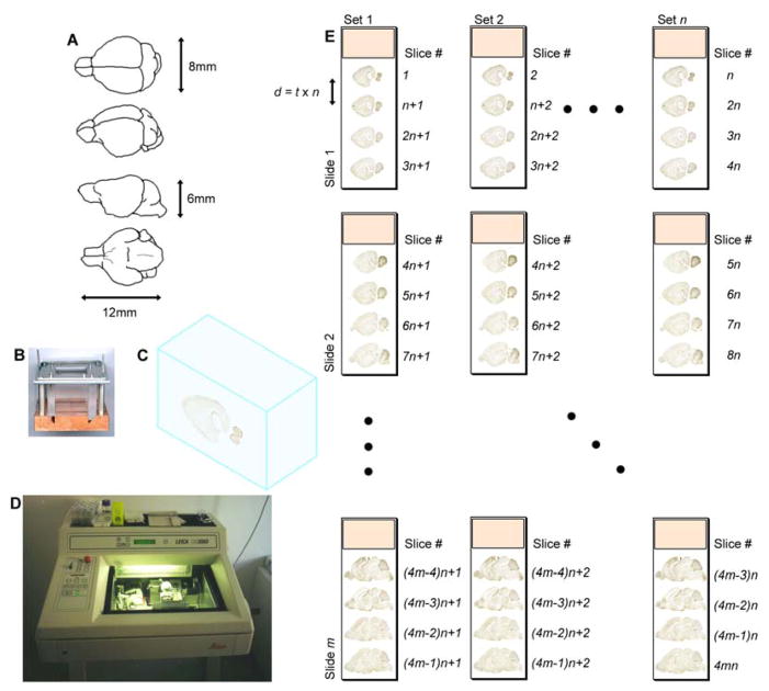
P7 brains extracted from the C57BL6 mouse strain are approximately 6×8×12 mm in size (Fig. 2A). Each fresh mouse brain is placed into a freezing chamber consisting of a 5×5 cm copper base, transparent Plexiglas sidewalls, and an aluminum top bracket held in place by stainless steel rods and a pair of clamps (Fig. 2B). The chamber sits on top of a slab of dry ice while the chamber is filled with O.C.T. cryomount medium. During this process, the brain is aligned visually to keep the brain axes parallel to the walls of the freezing chamber. This creates a frozen block containing the stereotaxically aligned tissue (Fig. 2C). The blocks can be stored indefinitely at −80° C. Frozen blocks must be moved to a −20° C freezer prior to sectioning in order to equilibrate to the temperature inside of a cryostat. Brains are sliced sagittally (i.e., from the left lateral side to just past the midline) into 25 μm-thick tissue sections using the cryostat (Fig. 2D). Serial tissue sections are placed onto alternating sets of slides (Fig. 2E). With eight sets collected for each brain, the resulting distance between tissue sections within a set is 200 μm. Sections are fixed in 4% paraformaldehyde, acetylated, and dehydrated for further storage at −80° C.

Fig. 2.

Tissue preparation protocol for high-throughput in situ hybridization. (A) Basic dimensions and shape of the P7 mouse brain. The third image from the top shows a sagittal view. (B) The empty freezing chamber into which the mouse brain is placed consists of a 5 × 5 cm copper base, transparent Plexiglas sidewalls, and an aluminum top bracket held in place by stainless steel rods and a pair of clamps. This chamber was developed at the Max Planck Institute of Experimental Endocrinology in Hannover, Germany. (C) The frozen block containing the mouse brain. (D) Cryostat used for slicing the mouse brain at a consistent thickness, t = 25 μm. (E) Slices are alternately distributed into n different sets, with each set consisting of m slides. During ISH, a specific gene probe is assigned and applied to an entire set. Distance, d, between slices within a set is t × n.

2.1.3. High-throughput in situ hybridization

High-throughput (HT) ISH was developed as a method to perform large-scale analyses with a daily throughput of 196 standard 25mm×75mm glass slides with four tissue sections per slide (24). HT-ISH is based upon the catalyzed reporter deposition (CARD) signal application protocol that enhances sensitivity of non-radioactive ISH (25). Reaction steps – prehybridization, hybridization and signal amplification/detection – are performed in a flow-through chamber (200 μl) into which solutions are added in parallel with an automated Tecan Genesis pipetting robotic solvent delivery system. Hybridization is carried out with digoxygenin (DIG)-tagged riboprobes. To visualize expression, DIG-tagged riboprobes are detected with an anti-DIG antibody to which peroxidase is coupled. Peroxidase is used to activate a tyramine–biotin conjugate, which is subsequently covalently attached to proteins in the vicinity of the anti-DIG antibody. Then biotin is detected with a streptavidin–alkaline phosphatase-based color reaction (26), resulting in the formation of blue-colored precipitate crystals localized to the cell.

2.1.4. Microscopy

Slides are cover-slipped and digitally scanned via a CCD camera at 1.6 μm/pixel, a magnification appropriate for detecting individual neuron cell bodies which are approximately 10 μm in diameter, using a custom-made automated Leica (Wetzlar, Germany) bright-field compound microscope with a motorized stage that holds up to 8 slides (4). Individual 24-bit color images (each 575×575 pixels in size) are stitched together automatically to produce a single mosaic image approximately 10,000×5,000 pixels in size representing the entire section, a step that relies on pre-calibrated image placement in the mosaic and the accurate translation of the motorized stage. Images are automatically cropped and stored as Red-Green-Blue (RGB) Tagged Image File Format (TIFF) files with Lempel Ziv Welch (LZW) lossless compression using Adobe Photoshop (Adobe Systems Incorporated).

2.2. Detection of gene expression

Different types of neurons and other cells perform a variety of functions. A necessary component of gene expression characterization is cell-based detection of gene expression. For example, a small population of cells could have the same total amount of transcript, but the transcript could be unevenly or evenly distributed across the cells. For these two situations, the functional relevance is potentially substantially different. Dye-based ISH has been shown to quantitatively correlate with transcript levels as detected by microarrays (27). The Celldetekt system for fast accurate automated classification of cellular gene expression described in this section has been validated against visual classification of cellular gene expression as well as calculations of dye content at higher magnifications (28). The motivation for this semi-quantitative approach is based on the limits of resolving small differences in levels of detected precipitate at the resolution at which data is collected, as well as the limited means for validating the significance of such small changes.

2.2.1 Categories of signal strength

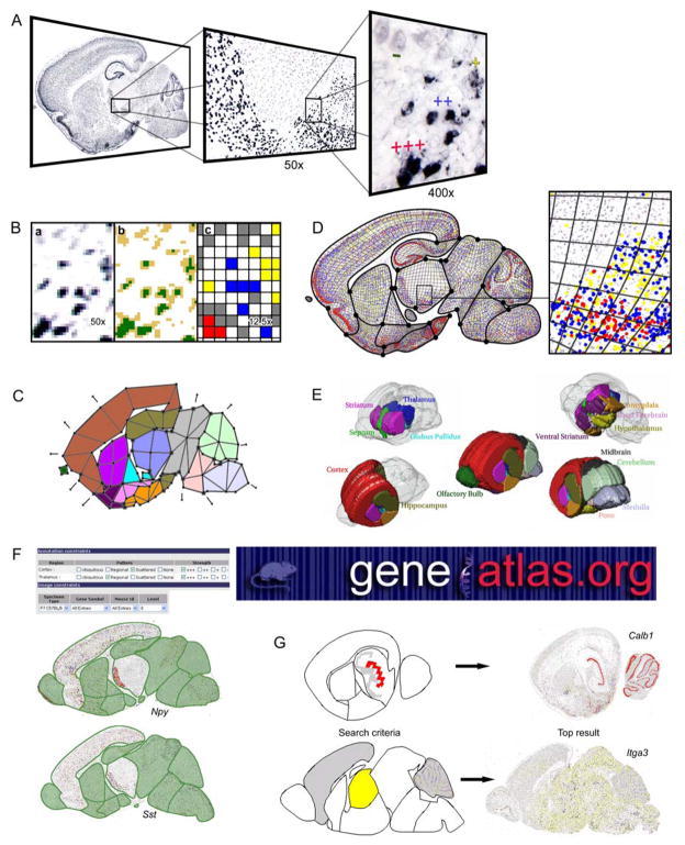
The quantity of cellular precipitates as a result of the non-radioactive ISH increases with the number of detected transcripts (Fig. 3A). Visible levels of gene expression strength range from cells with no detectable expression to cell bodies completely filled with dye precipitate. The range of visibly observable and distinguishable expression strengths is divided into four categories: strongly expressing cells filled with dye precipitate (+++), moderately expressing cells partially filled with precipitate (++), weakly expressing cells with scattered minute particles of deposit (+), and cells with no detectable precipitate (−) (10, 28). Having detected multiple levels of gene expression signal strength enables flexibility in selecting the strength threshold for quantitative comparisons (3), as well as the potential for analyses that incorporate multiple levels of signal strength including scoring systems for clustering gene expression patterns (14).

Fig. 3.

Illustration of automated annotation process for the P7 mouse brain. (A) Cnr1 expression as collected by HT-ISH protocols with strength of expression labeled at high magnification. HT imaging is at 100x. (B) Automated expression strength classification using Celldetekt. (a) Original Cnr1 at 50x as followed by (b) intensity thresholding results in (c) cell signal strengths marked by color in a 12.5x image. (C) Standard deformable map number 4 shown here absent of subdivisions. (D) After registration, the quantified cellular gene expression data is attached to the quadrilaterals in the subdivided standard mesh. (E) The 15 major anatomical regions of the P7 mouse brain are shown here in a 3D stack of the standard maps. (F) Once in the context of the atlas and patterns have been automatically been detected, a textual search at the website www.geneatlas.org can be used to find genes of interest. In this example, two genes are found matching the criteria of strong scattered expression in the cortex and strong regional expression in the thalamus. (G) Sophisticated graphical searches take advantage of the subdivision mesh characteristics and web-friendly display to allow users full control of the region(s) of interest in a search. Users can define their own regions of interest and levels of expression in each region, or they can use genes already in the database as search criteria, or a combination of these mechanisms.

2.2.2 Signal detection

Gene expression signal detection and categorization is implemented as Celldetekt, a python script (http://www.python.org/) utilizing the Python Imaging Library (http://www.pythonware.com/) that automatically identifies pixels representing precipitate and then classifies clusters of pixels by size (28) (Fig. 3B). A fixed threshold method identifies pixel type using two user-provided threshold values, t₁ and t₂, with Green-channel pixel intensities less than t₁ assigned to dye precipitate, and remaining Grey intensities up to t₂ designated as cellular areas without precipitate (Fig. 3Bb). Unassigned pixels indicate the absence of cell bodies. Although fixed throughout a given image, thresholds can be adjusted between sets of data to compensate for variations in the HT-ISH protocol that may result in staining differences for either the precipitate or the background.

Detecting cells is accomplished using a sliding window technique. A series of square windows traverse the entire image marking the locations where the signal filled the window. The first 3×3 pixel window approximates the average size of a neuron cell body (~10μm in diameter) in the image scaled to 3.3 μm/pixel. At locations where every pixel within the window is precipitate signal, the point is marked as a cell with +++ gene expression. After scanning through the entire image, signal near the +++ detected cells are removed by a circular 7 pixel diameter mask to prevent subsequent re-detection. This sliding window procedure is repeated with a 2×2 pixel window to detect ++ cells and then a 1×1 pixel window to detect + cells. Cells without any dye precipitate are next located using the same protocol as for the precipitate-containing cells. Clusters of cells are segmented into approximately cell-sized units by reducing the image size another 25% to produce a digital false color map with each pixel representing one cell color-coded by the expression strength of the cell (Fig. 3Bc).

2.3 Atlas construction

To provide a single common spatial context for gene expression images, a series of two-dimensional (2D) deformable maps of P7 mouse brain sagittal sections is created utilizing the 11 sagittal tissue slices comprising Valverde’s P7 mouse brain atlas (29) as a guide (3, 30). These 2D maps corresponding to 11 standard tissue sections and defining 15 anatomical structures (Fig. 3E) constitute an atlas for the mouse brain. Subdivision meshes (22) are used to represent each map. Each subdivision mesh consists of a coarse mesh of quadrilaterals plus a set of subdivision rules for generating increasingly fine quadrilateral meshes that smoothly approximate the initial coarse mesh (for a detailed description, see the concurrent article). Modeling anatomical regions entails tagging each quadrilateral in the coarse mesh by its associated anatomical region (Fig. 3C). By applying special subdivision rules to edges and vertices shared by quadrilaterals with different tags, the fine mesh accurately models the smooth boundaries between distinct anatomical regions. In addition to precisely fitting the boundaries between major regions, small internal anatomical sub-regions are accurately localized (3).

2.4. Atlas-based registration

Registering the atlas onto the ISH images undergoes the standard two-step procedure, starting with a global affine transformation to account for shifting and rotations during image collection, followed by a local per-vertex deformation to account for anatomical variations (3, 30, 31). The general methodologies for performing the two steps are introduced in the concurrent article in a data-independent manner. Here, we detail the procedures and modifications specifically for registering ISH images.

2.4.1 Image selection

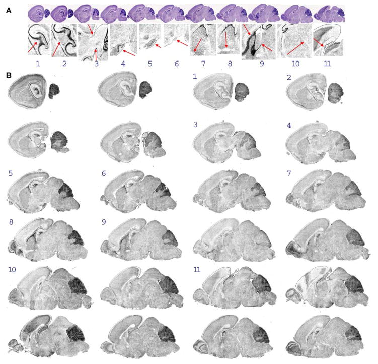
Images that best match the anatomical topology of the 11 standard tissue sections (see 2.3) are selected from the collection of digitized images (32). First, for each standard section, a key anatomical feature was identified (Fig. 4A). Then, an automated program was developed to perform cross-correlation of the key anatomical features to all of the histogram-normalized images of the data set in order to identify which tissue sections were most likely to contain the features (Fig. 4B). To facilitate visual validation – and if necessary a user-decided correction of this step – the implementation displays thumbnail representations of all of the images in the dataset along with the computed best assigned match to each standard. Ultimately, for each standard tissue section, one unmodified image from the dataset is selected even in cases where two images may appear to match a standard tissue section.

Fig. 4.

Automated image selection program output. (A) The header at the top of the image output indicates which anatomical features in the standard sections to look for during visual confirmation of image selection. These are the same features as used during the calculation of the best match via cross-correlation. (B) Main output displays image thumbnails of all 24 ISH data images along with numbers that label the images as best matching a particular standard section.

2.4.2 Initial global registration

To fit a given section with the subdivision atlas, the mesh is first deformed onto the tissue using global affine transformation consisting of translations and rotation. The deformation is computed via standard Principle Component Analysis on the atlas and on the detected tissue on each image (30).

2.4.3 A statistical atlas for local deformation

After global affine alignment to an image, the atlas needs to be further adjusted to account for local differences in anatomical shapes between the atlas and the image. This entails repositioning each vertex in the coarse subdivision mesh, which can be solved by formulating a least-square minimization problem whose goal is to reduce the fitting error between the atlas and the image while maintaining a low geometric distortion of the atlas (31).

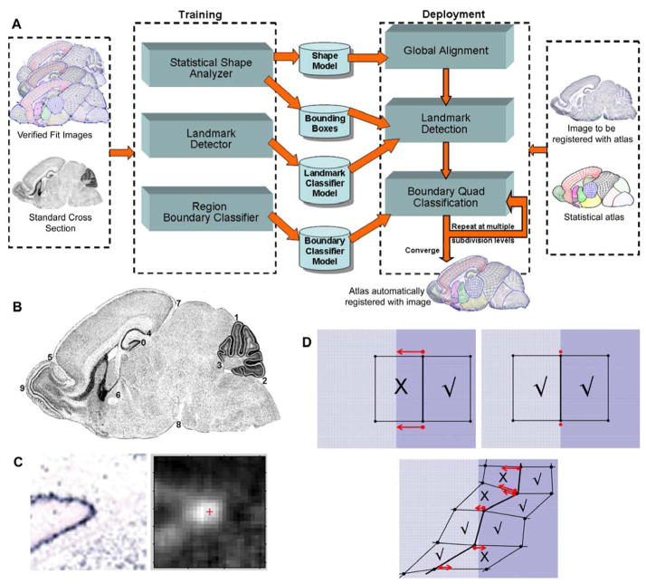
To more accurately fit an ISH image, we have augmented the atlas with statistics of the shape of the regions, the location and appearance of selected anatomical landmarks, and texture variation at anatomical region boundaries (31). Specifically, the subdivision mesh, Ai, for each of the 11 standard cross sections is associated with a triplet such that A_i = (S_i, L_i, B_i), where S_i represents the subdivision mesh shape, L_i describes the position and optimal texture features for selected anatomical landmarks, and B_i models the appearance at the boundaries of anatomical regions. This hybrid statistical framework is the key technology for highly refined automated registration (Fig. 5A). Unlike other image registration methods, for example (33, 34), this is the first approach to combine subdivision surfaces with landmark deformation, where landmarks can be both points and boundary contours.

Fig. 5.

Automated registration. (A) Flow-chart of automated registration steps. (B) Example of 10 landmarks displayed on a standard tissue section. (C) SVM probability estimates for pixels around landmark 0. (D) Classification of mesh elements at a boundary between regions. X marks misclassified quadrilaterals, with arrows indicating how the boundary edge will automatically displace towards the misclassified element. Source: (31) (© 2007 IEEE).

S_i is a representation of the shape at multiple subdivision levels where the shape at each subdivision level is expressed as a linear combination of the mean shape and shape vectors obtained during training. These shape vectors are the eigenvectors corresponding to the eigenvalues that represent the principal modes of shape variation.

L_i captures statistical information about the location and appearance of selected landmarks. These landmarks are locations in the image that have a fairly consistent shape and appearance (Fig. 5B). External boundary landmarks are points of extreme curvature along the outer boundary of the brain section. Each boundary landmark is associated with its average and variance of a set of parameters including mesh location and curvature of the boundary at the landmark. Internal landmarks are anatomical subregions generally recognized by a distinctive change in cell density, such as a cross-section of the anterior commissure fiber tract. Each internal landmark is associated with its average and variance of a set of parameters including mesh location and texture-based classification features acquired from training datasets.

B_i represents the texture features inside the mesh quadrilaterals at the region boundaries. A boundary segment is the anatomical boundary curve between two regions. For each boundary segment, a class of optimized texture features are defined for classifying each side of the segment.

2.4.4 Training the statistical atlas

Training the statistical framework is a one-time step performed using a series of mouse brain gene expression images on which landmarks are marked and the subdivision meshes are expertly fitted manually (31). A template is placed on each landmark and on surrounding areas to extract texture features, including the moments of an ordered set of sub-windows within the template, responses of Gabor filters, and Laws’ Texture energy measures (35). The texture features are normalized and discretized using Fayyad and Irani’s Minimum Description Length criterion (36). Information Gain Ratio is used to rank the features and an optimal set of features for discriminating between the landmark and its surrounding area is obtained in a Forward Selection process. A Support Vector Machine (SVM) classifier (37) is then constructed to distinguish the landmark from its neighbors using the selected optimal features. Similarly, texture features are extracted from quadrilaterals at multiple mesh subdivision levels on opposite sides of anatomical boundaries and SVM classifiers are built for each boundary segment as with the landmarks. The number of training samples used is dependent upon the information redundancy of the training dataset. For our experiments we chose training samples that captured a variety of information. Specifically, 30 images were used for our original training set to generate the results in this paper. The SWM reduces the possibility of over-fitting by finding the hyperplane that maximizes the separation between two classes in multi-dimensional space. Over-fitting was not observed in the dataset that we used.

2.4.5. Registration using the statistical atlas

Subdivision-based atlases are automatically deformed to new gene expression images using an energy minimization framework (described in the concurrent article). After affine alignment, texture features are extracted from pixels within the bounding boxes and the SVM classifier is applied to classify the pixels (Fig. 5C). The pixel with the highest probability estimate surrounded by similarly high estimates is selected as the landmark. Texture features are extracted from quadrilaterals on both sides of anatomical region segments, and the SVM classifier for each specific segment classifies these. The region boundaries are appropriately adjusted to match the classification in the model (Fig. 5D). The process is repeated at multiple levels of subdivision (31).

The statistical atlas for registration utilizing shapes, landmarks, and boundary texture features enables local deformation that accurately captures the shape of brains. All the shapes in our mouse brain datasets have been successfully registered using this approach (31). However, additional training of the registration framework may be necessary as the database of mouse brains expands. This problem can be addressed by adding automatically-fitted images that have been manually verified to the training set.

2.5. Data storage

After registering a standard subdivision mesh to a tissue section image, each cell-based data point generated by Celldetekt (see 2.2.2) is associated with the mesh quadrilateral in the overlying deformed atlas at a fine subdivision level (Fig. 3D). This association, the image of the tissue section, and all other metadata are stored on the www.geneatlas.org host web-server, an online database built using mySQL and Java Servlet pages (3, 30). The association is stored as an array of floating point values, each being the average gene expression level within a quadrilateral of the deformed atlas, with additional multi-resolution summaries used to accelerate region-based queries (30). The image stored is an RGBA image at 12 μm/pixel resolution with the gene expression signal Celldetekt information encoded in the A channel. The image is saved as PNG format (www.libpng.org) which was selected because it is a widely supported lossless-compression image format with no patent-based restrictions on usage (38). Associated metadata include the gene name, gene ID, sagittal plane location, status of mesh-fitting process, mouse identification number, slide number, and links to the high resolution raw image data at GenePaint.org (10).

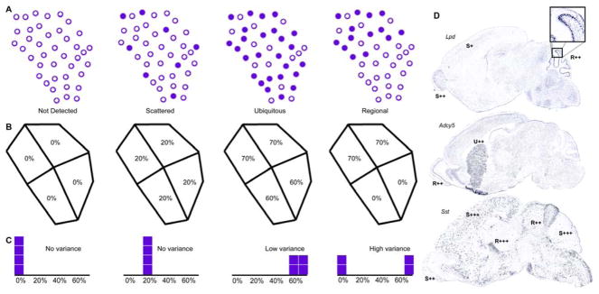
2.6. Pattern annotation

ISH patterns in major anatomical structures are customarily annotated in a textual manner by classifying the expression patterns as ubiquitous (U), scattered (S), regional (R) or not detected (ND) (39). With spatial gene expression information now accurately segmented into major anatomical regions by the registered atlas, pattern annotations are automatically generated for each region (Fig. 6) (39). The two key components of an expression pattern are the number of cells expressing and the distribution of that expression within a structure. Each structure type possesses its own unique substructure arrangement, requiring the parameters used in the annotation algorithm to be assigned on a structure-by-structure basis (Table 1). The classification of ND is assigned when the total percentage of cells expressing in the structure is less than χ.

Fig. 6.

Pattern types and basic pattern assessment. (A) Illustrations of the four types of patterns are shown. Filled circles are expressing cells, and empty circles are non-expressing cells. “Not detected” has no cells expressing. “Scattered” has a small percentage of cells expressing and evenly distributed throughout the structure. “Ubiquitous” has a large percentage of cells expressing and evenly distributed throughout the structure. “Regional” has an uneven distribution of cells. (B) The structure in (A) is divided into 4 quadrilaterals with the percentage of cells expressing shown in each one. (C) Histograms of the distribution of the percentage of cells expressing in each quadrilateral are shown for each example. An even distribution of expression across a structure clusters the values on the histogram. This corresponds to a low variance. Values spread out across the histogram create high variance, which thus indicates differences in expression levels amongst the structure’s substructures. (D) Automatically generated annotations for particular regions are displayed for three different genes: adenylate cyclase 5 (Adcy5), lipidosin (Lpd), and somatostatin (Sst).

Table 1.

Pattern annotation variables listed by structure.

Structure	α	β	γ	δ	χ
Cortex	0.7	0.7	50.00%	2.00%	1.00%
Cerebellum	0.72	0.72	45.00%	2.00%	1.00%
Striatum	0.7	0.72	40.00%	4.00%	1.00%
Basal Forebrain	0.7	0.7	50.00%	3.50%	1.00%
Amygdala	0.7	0.7	57.00%	2.00%	1.00%
Hippocampus	0.73	0.5	50.00%	3.70%	1.50%
Hypothalamus	0.7	0.5	50.00%	1.80%	1.00%
Thalamus	0.55	0.45	50.00%	2.00%	0.90%
Olfactory Bulb	0.65	0.65	50.00%	3.50%	1.00%
Midbrain	0.65	0.7	47.00%	3.00%	0.80%
Pons	0.7	0.7	45.00%	2.00%	1.00%
Medulla	0.7	0.7	45.00%	2.00%	1.00%
Ventral Striatum	0.9	0.7	50.00%	2.00%	1.40%
Globus Pallidus	0.55	0.7	50.00%	2.00%	1.00%
Septum	0.7	0.7	50.00%	3.00%	1.00%

U is assigned to structures in which the total percentage of cells expressing is greater than γ. Between χ and γ, the classifications R and S are differentiated by examining the scaled weighted deviation (SWD) in the percentage of gene expression across the quadrilaterals within the region. SWD is weighted during calculation by the number of cells in each quadrilateral, and scaled by the total percentage of expression. Regional patterns are indicated by higher deviations in the distribution of expression across the structure at subdivision level 1. For SWD greater than α, R is assigned; otherwise, S is assigned. At very low amounts of expression (between χ and δ), deviations are calculated at subdivision level 0 and compared to β. In cases where a particular structure exhibits multiple specific patterns, the most dominant is assigned. This is accomplished by calculating pattern separately for each of the expression strengths and selecting the strongest detected pattern.

2.7. Interactive knowledge discovery applications

2.7.1. Textual queries

Textual queries allow users to search for genes by specifying a set of search criteria based on expression pattern and strength for each major anatomical structure of interest (32). In this interface, each of the 15 major anatomical structures can be restricted to a particular pattern or set of patterns by selecting one or more of the corresponding buttons (Fig. 3F). Data associated with the images that can be used to define the query include the specimen age and strain, gene symbol, mouse ID, standard section plane number, fitted status, GenePaint.org identification number, gene accession number, and Entrez Gene identification number.

2.7.2. Graphical queries

The graphical query is similar to the textual query in that genes are searched based upon their expression pattern; but in this case, the graphical interface allows users to define unique regions of interest by selecting the specific set of quadrilaterals of interest at any level of subdivision (Fig. 3G) (3). After defining the region, users specify the expression strength quad-by-quad as strong, medium, weak, or none. Alternatively, the expression strength distribution of genes in the database may be used as the search criteria for this user-defined region. Queries compare expression patterns using an L₁ or χ² norm of the average gene expression level on a quad-by-quad basis, and sum up the results to calculate an error value representing the difference between two gene expression patterns.

2.7.3. Comparative analysis

Representing gene expression patterns quantitatively in a common coordinate system facilitates the comparison of cellular gene expression strength and distribution in two different experimental states (3). Control and experimentally modified specimens are simultaneously subjected to HT-ISH for a gene of interest, as any changes in conditions (e.g., probe lengths, reaction detection durations) can affect signal amplification, which in turn augments the quantity of precipitate deposited. Celldetekt is performed on imaged specimens and the appropriate standard map is registered to all tissue sections containing the region(s) of interest. The quadrilaterals in the standard mesh overlying the region of interest are selected. The cellular quantitative gene expression values are then extracted from these regions and statistically compared. In this way, blind comparative analysis is performed using a systematic definition of the region. Comparisons can be made using either the percentage of cells in a region expressing the gene at a particular strength, or by simply comparing the total number of cells in that region expressing above a user-determined strength threshold.

2.7.4. Cluster analysis

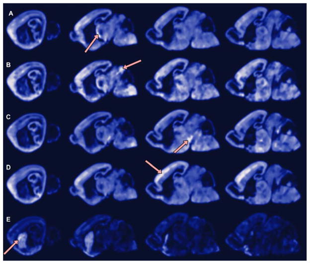
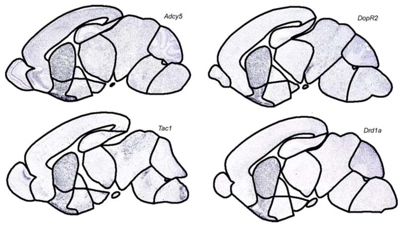
HT-ISH creates an abundance of information in regards to how genes express with a high spatial resolution. With an organ such as a brain that has many different subregions, the tissue itself becomes a natural laboratory for expression analysis since the subregions each have their own functions and set of cell types (14). When expression patterns for many genes are collected in this fashion and mapped into a common coordinate system, two basic categories of questions can be answered by clustering techniques. The first category asks what are the subregions of the brain as defined by gene activities, and what are the gene-based relationships between disconnected regions (Fig. 7). The second seeks to understand which genes tend to work with each other, (i.e., what are the genetic modules (Fig. 8)). To answer these, a k-means clustering algorithm can be applied. The iterative process begins after random assignment of points to k groups. During each cycle, the centroid (i.e., mean) of each group is calculated and points are reassigned to the closest centroid. Once the local minima of total distance between points and centroid is found, the result is stored and the whole process repeats with the points randomly assigned to groups again. After multiple iterations, the result that minimizes total distance between points and centroids is kept. In the case of partitioning the brain, each of the M quadrilaterals is represented as a point in N-dimensional space with N equal to the number of genes in the dataset. The value in each dimension is the percentage of cells either moderately or strongly expressing for that gene in the quadrilateral. The kcluster command from the open source Pycluster python package (40) clusters the points with Euclidean distance applied to score distances from points to centroids. Genes are clustered into groups by using the same technique as for the anatomical subregions, but on the transpose of the point matrix. In this case, the N-dimensional space has N equal to the number of quadrilaterals, and the number of M points is the number of genes.

Fig. 7.

Detecting spatial co-expression. A point is selected and the volume of the brain is locally evaluated for likelihood of expression when the selected point expresses. Standard cross-sections 2, 6, 9, and 10 shown (left column to right column). Positions of interest, indicated by the red arrows, are in the following anatomical structures and substructures: (A) the reticular nucleus in the thalamus; (B) the inferior colliculus of the midbrain; (C) the substantia nigra in the midbrain; (D) layer IV of the somatosensory cortex; and (E) the striatum.

Fig. 8.

Example gene cluster. Clustering genes based on their expression throughout the brain is one method that can identify genes that co-express and perhaps take part in the same gene network. In this example, 100 genes were clustered into 10 groups using k-means clustering. Displayed in this figure is one of the 10 groups. This group contains four genes, each of which generally expresses more in the striatum than in other anatomical locations, suggesting a potential relationship between these four genes.

2.8. Extending pipeline to 3D

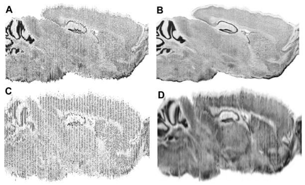
We have begun the process of extending this pipeline for automated atlas-based annotation of gene expression patterns to 3D datasets. One of the primary challenges in such extension is to create a 3D image volume from a stack of 2D ISH images, which is key to subsequent atlas construction, registration, and spatial queries (41, 42). However, the sectioning distortion resulting from ISH experiments yield artifacts when the images are simply stacked together. As an example, Fig. 9A shows a synthetic sagittal cut through the middle of a stack of coronal ISH Nissl stained sections. Note that the cut image is highly discontinuous due to the sectioning distortion that varies randomly from one slice to the next.

Fig. 9.

(A) Virtual sagittal cross-section through a stack of coronal images aligned only using rigid-body transformations (i.e., translations and rotations) reveal 2D distortion introduced during sectioning. (B) Virtual section reconstructed using our warping method. Synthetic sagittal section of stacked coronal sections of (C) raw ISH images and (D) after normalizing gene expression signals and warp-based reconstruction.

To address this challenge, we developed an elastic deformation technique based on dynamic programming that smoothly migrates each pixel on a slice to the average location of the corresponding pixels on multiple neighboring slices (43). The result when applied onto a stack of histological sections is a 3D image volume where any cut exhibits a smooth appearance (Fig. 9B). To apply the method onto gene expression images, normalization of gene expression signal is required for HT-ISH datasets where up to eight different genes will be collected from the same mouse brain by alternating the sections (Fig. 9C). To this end, expressing and not-expressing cells are detected using Celldetekt (28), converting binary images of detected cells to cell density using a Gaussian blur, and applying linear histogram normalization. On these normalized images, the warping algorithm can compute the necessary transformations to remove much of the local sectioning deformations to produce a volume suitable for automated volumetric atlas registration (Fig. 9D).

3. Concluding Remarks

Discovering which genes are active in different cell populations of the brain can significantly expand the knowledge of how gene products interact as well as how they affect biological processes and human disease. Automated atlas-based annotation provides a critical step in harnessing the terabytes of data generated by HT-ISH. The method described in this paper provides a straightforward method to perform interactive knowledge discovery of spatial gene expression datasets. Normally, the biggest challenge in this process is how to normalize in space the location of gene expression from different datasets. Due to the relatively small number of handles controlling the shape of a subdivision atlas – a prime advantage subdivision possesses over other atlas-based registration approaches – the approach described here allows an extremely high level of registration precision as these handles control the explicit boundaries between major anatomical regions, while the subdivision mesh smoothly interpolates the interior of the regions. This enables a variety of knowledge discovery applications that rely on precise registration, such as quantitative comparative analysis of gene expression in small anatomical regions across the mouse brain (3, 12–14). The 2D approach is limited to some extent by the slight variation in slicing angles during data production, as well as the need to fit multiple meshes per brain. This requirement for image slice angle to be well-aligned with the plane of the standard is the greatest challenge for this method, as poorly sliced data becomes unusable. With the future development of a 3D subdivision atlas, this challenge can be overcome and the overall pipeline can become even more efficient.

References

- 1.Albrecht U, Lu H-C, Revelli J-P, Xu X-C, Lotan R, Eichele G. In: Human Genome Methods. Adolph KW, editor. CRC Press; Boca Raton: 1997. pp. 93–119. [Google Scholar]
- 2.Boguski MS, Jones AR. Nat Neurosci. 2004;7:429–33. doi: 10.1038/nn1232. [DOI] [PubMed] [Google Scholar]
- 3.Carson JP, Ju T, Lu HC, Thaller C, Xu M, Pallas SL, Crair MC, Warren J, Chiu W, Eichele G. PLoS Comput Biol. 2005;1:e41. doi: 10.1371/journal.pcbi.0010041. [DOI] [PMC free article] [PubMed] [Google Scholar]
- 4.Carson JP, Thaller C, Eichele G. Curr Opin Neurobiol. 2002;12:562–5. doi: 10.1016/s0959-4388(02)00356-2. [DOI] [PubMed] [Google Scholar]
- 5.Heintz N. Nat Neurosci. 2004;7:483. doi: 10.1038/nn0504-483. [DOI] [PubMed] [Google Scholar]
- 6.Lein ES, Hawrylycz MJ, Ao N, Ayres M, Bensinger A, Bernard A, Boe AF, Boguski MS, Brockway KS, Byrnes EJ, Chen L, Chen L, Chen TM, Chin MC, Chong J, Crook BE, Czaplinska A, Dang CN, Datta S, Dee NR, Desaki AL, Desta T, Diep E, Dolbeare TA, Donelan MJ, Dong HW, Dougherty JG, Duncan BJ, Ebbert AJ, Eichele G, Estin LK, Faber C, Facer BA, Fields R, Fischer SR, Fliss TP, Frensley C, Gates SN, Glattfelder KJ, Halverson KR, Hart MR, Hohmann JG, Howell MP, Jeung DP, Johnson RA, Karr PT, Kawal R, Kidney JM, Knapik RH, Kuan CL, Lake JH, Laramee AR, Larsen KD, Lau C, Lemon TA, Liang AJ, Liu Y, Luong LT, Michaels J, Morgan JJ, Morgan RJ, Mortrud MT, Mosqueda NF, Ng LL, Ng R, Orta GJ, Overly CC, Pak TH, Parry SE, Pathak SD, Pearson OC, Puchalski RB, Riley ZL, Rockett HR, Rowland SA, Royall JJ, Ruiz MJ, Sarno NR, Schaffnit K, Shapovalova NV, Sivisay T, Slaughterbeck CR, Smith SC, Smith KA, Smith BI, Sodt AJ, Stewart NN, Stumpf KR, Sunkin SM, Sutram M, Tam A, Teemer CD, Thaller C, Thompson CL, Varnam LR, Visel A, Whitlock RM, Wohnoutka PE, Wolkey CK, Wong VY, Wood M, Yaylaoglu MB, Young RC, Youngstrom BL, Yuan XF, Zhang B, Zwingman TA, Jones AR. Nature. 2007;445:168–76. doi: 10.1038/nature05453. [DOI] [PubMed] [Google Scholar]
- 7.Magdaleno S, Jensen P, Brumwell CL, Seal A, Lehman K, Asbury A, Cheung T, Cornelius T, Batten DM, Eden C, Norland SM, Rice DS, Dosooye N, Shakya S, Mehta P, Curran T. PLoS Biol. 2006;4:e86. doi: 10.1371/journal.pbio.0040086. [DOI] [PMC free article] [PubMed] [Google Scholar]
- 8.Neidhardt L, Gasca S, Wertz K, Obermayr F, Worpenberg S, Lehrach H, Herrmann BG. Mech Dev. 2000;98:77–94. doi: 10.1016/s0925-4773(00)00453-6. [DOI] [PubMed] [Google Scholar]
- 9.Ringwald M, Eppig JT, Begley DA, Corradi JP, McCright IJ, Hayamizu TF, Hill DP, Kadin JA, Richardson JE. Nucleic Acids Res. 2001;29:98–101. doi: 10.1093/nar/29.1.98. [DOI] [PMC free article] [PubMed] [Google Scholar]
- 10.Visel A, Thaller C, Eichele G. Nucleic Acids Res. 2004;32:D552–6. doi: 10.1093/nar/gkh029. [DOI] [PMC free article] [PubMed] [Google Scholar]
- 11.Gong S, Zheng C, Doughty ML, Losos K, Didkovsky N, Schambra UB, Nowak NJ, Joyner A, Leblanc G, Hatten ME, Heintz N. Nature. 2003;425:917–25. doi: 10.1038/nature02033. [DOI] [PubMed] [Google Scholar]
- 12.Gatchel JR, Watase K, Thaller C, Carson JP, Jafar-Nejad P, Shaw C, Zu T, Orr HT, Zoghbi HY. Proc Natl Acad Sci U S A. 2008;105:1291–6. doi: 10.1073/pnas.0711257105. [DOI] [PMC free article] [PubMed] [Google Scholar]
- 13.McGill BE, Bundle SF, Yaylaoglu MB, Carson JP, Thaller C, Zoghbi HY. Proc Natl Acad Sci U S A. 2006;103:18267–72. doi: 10.1073/pnas.0608702103. [DOI] [PMC free article] [PubMed] [Google Scholar]
- 14.Visel A, Carson J, Oldekamp J, Warnecke M, Jakubcakova V, Zhou X, Shaw CA, Alvarez-Bolado G, Eichele G. PLoS Genet. 2007;3:1867–83. doi: 10.1371/journal.pgen.0030178. [DOI] [PMC free article] [PubMed] [Google Scholar]
- 15.Yaylaoglu MB, Agbemafle BM, Oesterreicher TJ, Finegold MJ, Thaller C, Henning SJ. Am J Physiol Gastrointest Liver Physiol. 2006;291:G1041–50. doi: 10.1152/ajpgi.00139.2006. [DOI] [PubMed] [Google Scholar]
- 16.Bug WJ, Wong WW, Gustafson C, Johnson GA, Martone ME, Price DL, Rosen GD, Williams RW, Zaslavsky I, Nissanov J. IEEE EMBS Conference on Neural Engineering; Kohala Coast, Hawaii. 2007. [Google Scholar]
- 17.Christiansen JH, Yang Y, Venkataraman S, Richardson L, Stevenson P, Burton N, Baldock RA, Davidson DR. Nucleic Acids Res. 2006;34:D637–41. doi: 10.1093/nar/gkj006. [DOI] [PMC free article] [PubMed] [Google Scholar]
- 18.Ng L, Pathak SD, Kuan C, Lau C, Dong H, Sodt A, Dang C, Avants B, Yushkevich P, Gee JC, Haynor D, Lein E, Jones A, Hawrylycz M. IEEE/ACM Trans Comput Biol Bioinform. 2007;4:382–93. doi: 10.1109/tcbb.2007.1035. [DOI] [PubMed] [Google Scholar]
- 19.MacKenzie-Graham A, Lee EF, Dinov ID, Bota M, Shattuck DW, Ruffins S, Yuan H, Konstantinidis F, Pitiot A, Ding Y, Hu G, Jacobs RE, Toga AW. J Anat. 2004;204:93–102. doi: 10.1111/j.1469-7580.2004.00264.x. [DOI] [PMC free article] [PubMed] [Google Scholar]
- 20.Dong HW. The Allen Reference Atlas: A Digital Color Brain Atlas of the C57BL/6J Male Mouse. Wiley; 2008. [Google Scholar]
- 21.Paxinos G, Franklin KBJ. The mouse brain in stereotaxic coordinates. Academic; San Diego, Calif. London: 2001. [Google Scholar]
- 22.Warren J, Weimer H. Subdivision methods for geometric design: a constructive approach. Morgan Kaufmann; San Francisco: 2002. [Google Scholar]
- 23.Mazziotta J, Toga A, Evans A, Fox P, Lancaster J, Zilles K, Woods R, Paus T, Simpson G, Pike B, Holmes C, Collins L, Thompson P, MacDonald D, Iacoboni M, Schormann T, Amunts K, Palomero-Gallagher N, Geyer S, Parsons L, Narr K, Kabani N, Le Goualher G, Feidler J, Smith K, Boomsma D, Hulshoff Pol H, Cannon T, Kawashima R, Mazoyer B. J Am Med Inform Assoc. 2001;8:401–30. doi: 10.1136/jamia.2001.0080401. [DOI] [PMC free article] [PubMed] [Google Scholar]
- 24.Herzig U, Cadenas C, Sieckmann F, Sierralta W, Thaller C, Visel A, Eichele G. In: Novartis Foundation Symposium: Complexity in Biological Information Processing. Bock G, Goode J, editors. Vol. 239. John Wiley & Sons; Chicester: 2001. pp. 129–49. [DOI] [PubMed] [Google Scholar]
- 25.Bobrow MN, Harris TD, Shaughnessy KJ, Litt GJ. J Immunol Methods. 1989;125:279–85. doi: 10.1016/0022-1759(89)90104-x. [DOI] [PubMed] [Google Scholar]
- 26.Kerstens HM, Poddighe PJ, Hanselaar AG. J Histochem Cytochem. 1995;43:347–52. doi: 10.1177/43.4.7897179. [DOI] [PubMed] [Google Scholar]
- 27.Lee CK, Sunkin SM, Kuan C, Thompson CL, Pathak S, Ng L, Lau C, Fischer S, Mortrud M, Slaughterbeck C, Jones A, Lein E, Hawrylycz M. Genome Biol. 2008;9:R23. doi: 10.1186/gb-2008-9-1-r23. [DOI] [PMC free article] [PubMed] [Google Scholar]
- 28.Carson JP, Eichele G, Chiu W. J Microsc. 2005;217:275–81. doi: 10.1111/j.1365-2818.2005.01450.x. [DOI] [PubMed] [Google Scholar]
- 29.Valverde F. Golgi atlas of the postnatal mouse brain. Springer-Verlag; New York: 1998. [Google Scholar]
- 30.Ju T, Warren J, Eichele G, Thaller C, Chiu W, Carson J. In: Eurographics Symposium on Geometry Processing. Kobbelt L, Schröder P, Hoppe H, editors. Eurographics Association; Aachen, Germany: 2003. pp. 166–76. [PMC free article] [PubMed] [Google Scholar]
- 31.Bello M, Ju T, Carson J, Warren J, Chiu W, Kakadiaris IA. IEEE Trans on Medical Imaging. 2007;26:728–44. doi: 10.1109/TMI.2007.895462. [DOI] [PubMed] [Google Scholar]
- 32.Carson JP. Quantitative annotation and analysis of gene expression patterns with an atlas of the mouse brain. Baylor College of Medicine; Houston: 2004. [Google Scholar]
- 33.Bazin PL, Pham DL. Med Image Anal. 2008;12:616–25. doi: 10.1016/j.media.2008.06.008. [DOI] [PMC free article] [PubMed] [Google Scholar]
- 34.Shen D, Davatzikos C. IEEE Trans Med Imaging. 2002;21:1421–39. doi: 10.1109/TMI.2002.803111. [DOI] [PubMed] [Google Scholar]
- 35.Laws K. Textured Image Segmentation. University of Southern California; Los Angeles: 1980. [Google Scholar]
- 36.Fayyad UM, Irani KB. Machine Learning. 1992;8:87–102. [Google Scholar]
- 37.Vapnik V. The Nature of Statistical Learning Theory. Springer; Berlin: 2000. [Google Scholar]
- 38.Wiggins RH, 3rd, Davidson HC, Harnsberger HR, Lauman JR, Goede PA. Radiographics. 2001;21:789–98. doi: 10.1148/radiographics.21.3.g01ma25789. [DOI] [PubMed] [Google Scholar]
- 39.Carson JP, Ju T, Thaller C, Warren J, Bello M, Kakadiaris I, Chiu W, Eichele G. 26th Annual International Conference of the IEEE Engineering in Medicine and Biology Society; San Francisco, CA. 2004. [DOI] [PubMed] [Google Scholar]
- 40.de Hoon MJ, Imoto S, Nolan J, Miyano S. Bioinformatics. 2004;20:1453–4. doi: 10.1093/bioinformatics/bth078. [DOI] [PubMed] [Google Scholar]
- 41.Ju T, Warren J, Carson J, Eichele G, Chiu W, Bello M, Kakadiaris I. The Visual Computer. 2005;21:764–73. [Google Scholar]
- 42.Commean PK, Ju T, Liu L, Sinacore DR, Hastings MK, Mueller MJ. Journal of Digital Imaging. 2008 doi: 10.1007/s10278-008-9118-z. [DOI] [PMC free article] [PubMed] [Google Scholar]
- 43.Ju T, Warren J, Carson J, Bello M, Kakadiaris I, Chiu W, Thaller C, Eichele G. J Neurosci Methods. 2006;156:84–110. doi: 10.1016/j.jneumeth.2006.02.020. [DOI] [PubMed] [Google Scholar]