FAST MONTE CARLO SIMULATION METHODS FOR BIOLOGICAL REACTION-DIFFUSION SYSTEMS IN SOLUTION AND ON SURFACES

Abstract

Many important physiological processes operate at time and space scales far beyond those accessible to atom-realistic simulations, and yet discrete stochastic rather than continuum methods may best represent finite numbers of molecules interacting in complex cellular spaces. We describe and validate new tools and algorithms developed for a new version of the MCell simulation program (MCell3), which supports generalized Monte Carlo modeling of diffusion and chemical reaction in solution, on surfaces representing membranes, and combinations thereof. A new syntax for describing the spatial directionality of surface reactions is introduced, along with optimizations and algorithms that can substantially reduce computational costs (e.g., event scheduling, variable time and space steps). Examples for simple reactions in simple spaces are validated by comparison to analytic solutions. Thus we show how spatially realistic Monte Carlo simulations of biological systems can be far more cost-effective than often is assumed, and provide a level of accuracy and insight beyond that of continuum methods.

1. Introduction

Quantitative simulations of complex biological systems present difficult challenges. One primary issue is the choice of appropriate level of detail. At one extreme, atomic-level simulations of molecular structure require extremely short timesteps, generally on the femtosecond scale [23]. Hence, very large amounts of computer time are required to simulate very small amounts of cumulative “biological” time (e.g., nanoseconds). Parallel machines allow simulation of larger systems through spatial decomposition of atoms across processors, but to reach long “biological” times (e.g., milliseconds and beyond) one must introduce spatial simplifications and algorithms that can be run with longer timesteps. For example, groups of atoms or amino acids can be lumped together (coarse-grained or collective dynamics methods, respectively), and then the movements of the aggregates can be computed with simplified molecular mechanics algorithms [3, 8]. Another example is diffusion of ions in local (molecular) potential fields, e.g., ion channel permeation, using the Poisson–Nernst–Planck equation [5, 14]. At still higher space and time scales, however, detailed molecular structure must be omitted and alternative models and algorithms are necessary.

At cellular scales, finite numbers of molecules interact in complex spaces defined by cell and organelle membranes. To simulate stochastic cellular events with spatial realism at reasonable computational cost, we have previously introduced diffusion and chemical reaction algorithms that use Brownian dynamics for diffusion of individual molecules, ray-tracing of random walk motion vectors to detect collisions, ray-marching to propagate rays after collisions, and Monte Carlo probabilities to decide which collisions lead to reaction events [4, 18, 20]. In many respects our ray-tracing methods are similar to those used in photorealistic computer graphics, where rays of light are followed as they travel from light sources to strike objects, creating shadows and reflections. In principle, light rays are infinitely long and their intensity may be attenuated during travel. Chemical motion rays, however, have a finite initial length that represents a possible net displacement by diffusion, and the ray length must be decremented during tracing as necessary (ray-marching). When using this approach with Monte Carlo reaction probabilities and typical biological systems, individual timesteps often can be on the order of microseconds, and so biological times on the order of milliseconds to minutes are accessible.

We first developed these methods to simulate a specific instance of chemical signaling, diffusion, and reaction of discrete neurotransmitter molecules in synaptic spaces [4, 2, 18, 19, 20, 21, 22]. In its earliest form, our simulation program MCell supported only basic planar surfaces that represented simplified shapes of synaptic membranes [18]. Later we introduced arbitrary triangulated meshes to represent complex curved shapes (MCell version 2 [20, 21, 22, 7]). In all of these earlier studies, however, diffusing molecules reacted only with static molecules localized on surfaces. Thus, molecules diffusing in solution (volume molecules) could not react with each other, nor could surface molecules diffuse and react with themselves.

Most signaling and metabolic pathways, on the other hand, include interactions between various ligand molecules, receptors, enzymes, nucleic acids, etc., all of which may be moving in solution and/or in membranous structures. For example, the epidermal growth factor receptor (EGFR) pathway is critically important to growth, survival, proliferation, and differentiation of mammalian cells [11]. Membrane-bound EGFRs can bind diffusing extracellular ligand molecules, dimerize, autophosphorylate their tyrosine residues, and subsequently trigger a host of intracytoplasmic and intranuclear signaling network modules. Spatially realistic stochastic simulations of cellular networks therefore require new computational tools, and in this paper we introduce unique new MCell algorithms that allow one to model reactions between diffusing molecules in solution, on surfaces, or both. In section 2 we describe concepts and tools for the design of arbitrarily complex models using this new MCell version (MCell3), and in sections 3 and 4 we present and validate new algorithms and software design optimizations that can substantially reduce computational costs. Examples of these optimizations include scheduling of events based on molecular lifetimes, and variable time and space steps. Together with associated tools like DReAMM¹ for model development and visualization, these capabilities open broad new avenues for quantitative spatially realistic biological simulations.

2. MCell3 simulation design

As in previous versions, MCell3 uses a Model Description Language (MDL) to define simulation input conditions and user-requested output. The MCell3 MDL is similar to that for MCell version 2 [20], but in some areas has changed and expanded considerably. In brief, MDL files are human-readable text and typically are modular so that descriptions of mesh geometry, molecules, reactions, output, etc., can be split into separate files for easy editing. A full description is beyond the scope of this paper and will be presented elsewhere.

2.1. Meshes and mesh regions

For spatially complex models one of the biggest challenges is generation of the initial mesh objects, which may number in the hundreds or thousands. Two general methods can be used to create a set of meshes [22, 7]: reconstruction from segmented volumetric imaging data (e.g., serial electron micrographs or electron microscopic tomography), or direct output from CAD (computer-aided design) software. We presently make heavy use of the free CAD program Blender (www.blender.org), for which we have written plug-in modules so that meshes can be exported directly for use with MCell and DReAMM. DReAMM subsequently can be used interactively to define and visualize named subregions (subsets of triangles) on meshes, and to iteratively refine, simplify, extract, and merge subregions and mesh objects to optimize their use with MCell3. DReAMM can also be used to create sophisticated animations of MCell3’s visualization data output, but, again, a full description is beyond the scope of this paper and will be presented elsewhere.

Simple box-shaped mesh objects are created easily with the MDL, and can include arbitrary rectangular subregions on each side. MDL commands also can be used to copy, scale, rotate, and translate boxes and triangulated meshes to create large repeated structures. However, MCell3 does not perform constructive solid geometry operations to retriangulate resulting objects. Remeshing of this sort instead can be performed with other specialized software designed for that purpose (e.g., Blender). Each mesh triangle has a front and back face and if necessary is divided into surface molecule locations (triangular tiles) using barycentric subdivision (see [20] and Figure 4.2). Mesh elements can be reflective, transparent, or absorptive to some or all defined classes of diffusing molecules. Mesh geometry that changes shape within a single simulation is not supported explicitly, but, as with MCell version 2, simulations can be checkpointed and restarted using different meshes to produce geometric alterations. For example, we have previously used checkpointing and a series of meshes to simulate an expanding pore between a synaptic vesicle and a presynaptic nerve membrane [18, 20, 21].

Fig. 4.2.

Molecular encounters. (A) Surface molecules occupy tiles in a barycentric subdivision of a triangle. The molecule being tested (open circle) encounters other molecules (black circles) if they are in the three grid elements adjacent to it (shaded triangles). (B) Volume molecules (open circle) diffuse; when they strike a surface, they encounter any surface molecule present in that grid element (shaded triangle). (C) Diffusing volume molecule (open circle) encounters other volume molecules (black circles) in a cylinder of radius rint about its path of motion; molecules in the wrong direction, farther away than rint, or past the end of the motion are not encountered (gray circles). (D) Encounters made by a moving volume molecule (open circle) are blocked by surfaces (black line). Reactions occur at higher probability when their interaction area is reduced by a surface (right diagram) than when not (left diagram); reactions do not occur when the encounter is blocked by an intervening surface (center diagram).

2.2. Molecules

As introduced above MCell3 supports diffusing and reacting molecules in solution (volume molecules), as well as molecules in membranes (surface molecules). Volume molecules are defined by a user-specified name and a three-dimensional diffusion coefficient, while surface molecules are given a two-dimensional diffusion coefficient. Surface molecules occupy triangular tiles on surface mesh elements, diffuse by hopping from tile to tile (section 3.3), and can react with neighboring surface molecules (section 4.2). Volume molecules do not have solid physical dimensions, but for the purpose of intermolecular collision detection and reaction they do have an effective cross-sectional area (section 4.4). Molecules can be added to simulations in a variety of ways. Specified numbers or densities can be added to mesh objects or regions, or to arbitrary unions or intersections of volumes enclosed by mesh objects. Molecules can also be distributed randomly in ellipsoids or cuboids of arbitrary size and position. Addition of molecules can occur at regular intervals or at arbitrary times. Similar methods can also be used to select molecules at random and remove them from the simulation. Finally, it is possible to specify the explicit location and type of every molecule.

2.3. Reactions

Surface molecules are often used to represent transmembrane proteins. Such a protein in the cell membrane has distinct extracellular, intramembrane, and intracellular domains. Similarly, a protein in an organelle membrane has distinct cytoplasmic, intramembrane, and luminal domains. Thus membrane proteins have a real spatial orientation with respect to the surrounding diffusion spaces. Some bind and release ligand molecules on the same side of the membrane, while others transport ligands across the membrane (bind on one side and release on the other). In some cases they can also flip orientation periodically. In still other cases, they function as voltage- or ligand-gated transmembrane ion channels. Some typical biological examples include the following: sodium-potassium ATPase molecules, which exchange extracellular potassium for intracellular sodium while consuming intracellular ATP; sodium, potassium, or calcium channels; and G-protein coupled receptors, which bind extracellular and intramembrane ligands and interact with a wide variety of intracellular signaling molecules.

Our earlier MDL reaction syntax encompassed some of this geometric complexity [20], but the new MCell3 syntax is much more general and is also closer to standard (space-free) chemistry notation. For example,

$$\text{X}+\text{Y}\to \text{Z}$$

illustrates the MDL syntax for a reaction between two volume molecules that produce a third volume molecule. For reactions involving surface molecules, the spatial directionality is specified by assigning each species to a numbered orientation class. Matching absolute values of the numerical specifiers indicate that the species are in the same class. Within each class matching signs (+/+ or −/−) indicate that the species share the same relative orientation with respect to the surface, while opposite signs (+/− or −/+) indicate opposite orientation.

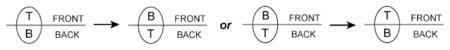
For example, consider the simple case of a transmembrane protein that can flip orientation. The diagram below shows a line that represents a mesh element seen in cross section, similar to a cross-sectional view of a membrane. The front and back of the mesh element are indicated, and could correspond to extracellular, cytoplasmic, or other regions of space depending on the context of the simulation. A single transmembrane protein molecule is shown by an oval with distinct spatial domains labeled T(op) and B(ottom). Again, the biological meaning of these domains depends on the context of the simulation. As shown in the diagram, the protein might begin a timestep in one of two possible configurations, T-FRONT or T-BACK, and subsequently flip to the opposite configuration:

(2.1)

Assuming the protein has been defined using a name of my_protein, the MDL syntax for this reaction might be

$$\text{my}\_\text{protein}\{1\}\to \text{my}\_\text{protein}\{-1\}$$ (2.2)

Since the numerical class specifiers have the same absolute value, the reactant and product are members of the same class. Hence, their relative orientations will be specified by the sign of the numbers. Since they have opposite signs, the molecule will flip orientation in the surface whenever the reaction occurs. As shown in (2.1) above, the molecule can start in either the T-FRONT or B-FRONT configuration, because the change in sign indicates a change in relative, not absolute, orientation. Thus, the same result would be obtained with

$$\text{my}\_\text{protein}\{-1\}\to \text{my}\_\text{protein}\{1\}$$ (2.3)

On the other hand

$$\text{my}\_\text{protein}\{1\}\to \text{my}\_\text{protein}\{2\}$$ (2.4)

indicates that the reactant and product are in different classes altogether. In this case their signs are ignored and the orientation of the product is assigned at random when the reaction occurs.

To make the syntax more compact, numerical class specifiers may be replaced with “tic marks.” In this case the number of tic marks on each species indicates the absolute value of its class, and the type of tic mark (apostrophe versus comma) indicates the sign. For example, in

$$\text{my}\_\text{protein}’\to \text{my}\_\text{protein},$$ (2.5)

the apostrophe and comma are part of the syntax, and (2.5) is equivalent to (2.2) and (2.3) above. On the other hand,

$$\text{my}\_\text{protein}’\to \text{my}\_\text{protein}”$$ (2.6)

is equivalent to (2.4) above.

To enforce absolute orientations and reactions occurring only on particular surfaces, a surface designation may be added to the reaction syntax. If a molecule and the surface are in the same class and have the same sign, then the T(op) of the molecule is aligned with the FRONT of the mesh element. For example, in

$$\text{my}\_\text{protein}’@\text{plasma}\_\text{membrane}’\to \text{my}\_\text{protein},$$ (2.7)

the comma again is a part of the syntax, and (2.7) specifies that the reaction can occur only if the initial configuration is T-FRONT (left-hand side of (2.1) above). In contrast,

$$\text{my}\_\text{protein},@\text{plasma}\_{\text{membrane}}^{’}\to \text{my}\_\text{protein}’$$ (2.8)

specifies that the starting configuration is B-FRONT (right-hand side of (2.1) above).

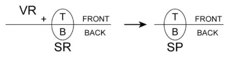
Similar concepts apply when volume molecules react with surface molecules. For example, given a volume reactant ( VR), a surface reactant ( SR), and a surface product ( SP),

$$\text{VR}’+\text{SR}’@\text{plasma}\_\text{membrane}’\to \text{SP}’$$ (2.9)

means that VR can react with SR when it is in the T-FRONT configuration on a mesh element that is part of plasma_membrane. The product SP will have the same orientation as SR and VR. In diagram form,

(2.10)

On the other hand

$$\text{VR}’+\text{SR}’\to \text{SP}’$$ (2.11)

means that VR can react with the T(op) of SR no matter what its configuration, T-FRONT or B-FRONT, or what surface mesh element it occupies. Whatever the directionality of the ensuing reaction, the product SP will be created with the same relative orientation as VR and SR.

Many other combinations are possible but will not be detailed here.² To see that this syntax covers all possibilities, note that the concept of relative orientation is reflexive (a molecule is oriented relative to itself), symmetric (if A and B share a relative orientation, then B and A do as well), and transitive (if A and B share a relative orientation, and B and C do as well, then A and C will also). Thus, “relative orientation” comprises an equivalence class containing reactants and products that must take on a specific relative orientation, and all reactants and products can be assigned to exactly one such class. The numerical class specifiers are exactly these equivalence classes. To easily confirm the behavior of directional reactions, DReAMM can display surface molecules as directional icons such as arrows or receptor protein glyphs. In addition, the FRONT and BACK of mesh elements can be given different colors and reversed as necessary.

2.4. Spatial subvolumes

In a naive collision detection algorithm, the search for intersections between M reacting molecules would scale as O(M²). In addition, the search for collisions between moving molecules and N mesh elements (triangles) would scale as O(MN), yielding approximately O(M(N +M)) overall and intractable run times for all but the smallest simulations. To accelerate performance, MCell3 partitions space into cuboidal spatial subvolumes (SSVs), similar to the method originally described for MCell version 2 [20]. Under optimal conditions, partitioning is adjusted so that each SSV contains only a small number of triangles and also a small number of molecules. The search for ray-triangle collisions during ray-marching thus can be limited to the current SSV, and simply begins again if the moving molecule crosses into an adjoining SSV. This effectively decouples execution time from N, the total number of triangles in the model.

The search for collisions between volume molecules is somewhat more complicated and requires new algorithms in MCell3 (section 4.4). Some molecules in surrounding SSVs may be closer to a current SSV boundary than the length of their effective radius, and therefore they extend into the current SSV. Hence, they must be identified and included in the list of potential collision partners. Under some conditions this requirement can be relaxed with little loss of accuracy (see Figure 4.3, section 4.4). Regardless, scaling of execution time approaches O(M) rather than O(M²), making simulations with 10⁵ or more molecules feasible even on single processors.

Fig. 4.3.

Volume reactions near surfaces. A pair of planes separated by a short distance d is filled with molecule I at a concentration of 1 mM. Molecules of J are introduced; J and I bind and unbind such that molecules of J should spend half of their time bound and half unbound. Plotted is the result of 40 simulations with an average of 100 binding/unbinding events each, comparing fixed $A=\pi r_{int}^2$ (large circles) to an exact calculation of A^★ (medium circles) or a time-saving extension where not only surfaces but also subvolume boundaries block reactions and reduce A^★ (small circles). The result primarily depends on the ratio d/r_int (x-axis); in this case, r_int was set to 5 nm (d ranged from 2 nm to 30 nm), J had a diffusion constant of 100 μm²/s, and I and the IJ complex did not diffuse. Error bars denote standard error of the mean.

2.5. Timesteps and scheduling

Previous versions of MCell were based on fixed timesteps. While the use of a fixed timestep simplifies the program design considerably, it also introduces several computational inefficiencies. First, unimolecular transitions (e.g., (2.1) above) are poorly served by fixed timesteps: states with short lifetimes cannot be represented accurately, while states with long lifetimes are visited many times before a state change occurs. Second, molecules with small diffusion coefficients (e.g., large proteins) may require a position update far less frequently than molecules with large diffusion coefficients (e.g., small ligands) to achieve the same relative spatial accuracy, and thus it is wasteful to update the slow moving molecules as often as the fast moving molecules.

To increase computational efficiency, we implemented a scheduling-based system in MCell3. The scheduler maintains a user-specified canonical timestep ΔT during the simulation, but allows an internal Δt to vary from molecular species to species. Thus, molecules that undergo rapid reactions can have a shorter Δt, while slowly diffusing molecules operate with a large Δt. This is accomplished by scheduling each molecule independently. At time T in the simulation, all events scheduled between T and (T + ΔT) occur, but strict temporal ordering is not enforced within each timestep. Molecule i of molecular species I maintains its own time t_i as well as the time Δu_i to its next unimolecular reaction (if applicable). The molecule diffuses for a species-specific timestep Δt_I, or longer if no reaction partners or geometry could affect it within that time, or for Δu_i if that is less than Δt_I. Bimolecular or surface reactions can happen during diffusion (e.g., (2.10) above), which is modeled as a constant-velocity transit. Products of the reaction are scheduled for their first movement at the time at which the encounter occurred. Nondiffusing molecules that undergo unimolecular transitions are immediately scheduled to undergo their next transition at time t_i + Δu_i, but can be interrupted if hit by a diffusing molecule with which they react. The simulation iterates over all molecules until t_i > (T + ΔT) for all i, and the simulation then advances T by ΔT and begins again.

3. Diffusion algorithms

In this section we present the theory and implementation of MCell3’s optimized algorithms for fast Monte Carlo simulation of diffusion in a volume or on a surface.

3.1. Unbounded diffusion

Suppose a molecular species is present at a concentration c(r, t) and is free to undergo random thermal motion in a fluid. The time evolution of concentration of that species is given by the diffusion equation

$$\frac{\partial c}{\partial t}=D{\nabla }_{\mathbf{r}}^{2}c,$$ (3.1)

where D is the diffusion coefficient of the molecule in that medium at that temperature. In a stochastic simulation we treat concentration as a collection of individual particles at precise locations, rather than represent it as a continuous function. In concept our strategy is as follows: For a given molecule, we use the diffusion equation to calculate the distribution of final positions for that molecule after a time Δt. We then pick a new specific position from that distribution, update the molecule’s position, and advance time by Δt. In practice, we accelerate this process enormously by precomputing a standardized distribution, storing it in memory as look-up tables, and then using random numbers to sample the tables for each movement [20].³

In particular, suppose that a single molecule is at the origin at time t = 0 and diffuses away with diffusion constant D. Then it can be shown from the diffusion equation that

$$c(\mathbf{r},t)\propto \frac{1}{{(4\pi Dt)}^{d/2}}{e}^{-\mathbf{r}·\mathbf{r}/4Dt},$$ (3.2)

where d is the dimensionality of the space in which diffusion is taking place (2 for surfaces, 3 for volumes). This concentration is radially symmetric, so r can be replaced by r = ||r||. It is also convenient to define the diffusion length constant $\lambda =\sqrt{4Dt}$. The probability density of final positions for the molecule then can be written

$$\rho (r,t)=\frac{1}{{\pi }^{d/2}{\lambda }^d}{e}^{-r^2/{\lambda }^2}.$$ (3.3)

To pick a radial distance for diffusion, one can pick a random variable X uniformly between 0 and 1 and solve

$$X=\text{cdf}(R,t)={\int }_0^R\rho (r,t)·\mid \partial S_r^d\mid ·dr$$ (3.4)

for R, where $\mid \partial S_r^d\mid$ is the surface area of a d-dimensional sphere of radius r; we set $\mid \partial S_r^1\mid =1$.

For three dimensions, the surface area is 4πr² so (3.4) becomes

$$X={\int }_0^R\frac{4\pi r^2}{{\pi }^{3/2}{\lambda }^3}{e}^{-r^2/{\lambda }^2}dr,$$ (3.5)

which can be solved for all values of λ by making the substitution r̃ = r/λ (r̃ was denoted by s in [20]). The solution to this dimensionless problem is

$$X={\int }_0^{\stackrel{\sim }{R}}\frac{4{\stackrel{\sim }{r}}^2}{\sqrt{\pi }}{e}^{-{\stackrel{\sim }{r}}^2}d\stackrel{\sim }{r}=\text{erf}(\stackrel{\sim }{R})-\frac{2}{\sqrt{\pi }}\stackrel{\sim }{R}{e}^{-{\stackrel{\sim }{R}}^2}.$$ (3.6)

As introduced above, we speed computation by solving this distribution for regularly spaced values of X when a simulation is initialized, and then store the resulting values in a look-up table held in memory (typically 1024 values). Thereafter, the run-time computation reduces to generation of a pseudorandom number, a table look-up for R̃, and a multiplication by λ to get the radial distance. Alternative methods mentioned above currently present no significant advantages. From here on, we will predominantly express diffusion distances in terms of the length-constant-normalized distance r̃ instead of the actual distance r.

The angle of travel is calculated separately from the distance; one can pick φ uniformly at random from [0, 2π) and pick θ in proportion to the circumference of the circle about the sphere at angle θ (equivalent to picking Y uniformly at random and solving $Y=\frac{1-cos\theta }{2}$ for θ). However, this approach is slow because it requires inverse trigonometric functions to be computed for each diffusion step. Once again we speed computation by precalculating a look-up table of random direction vectors, and then sampling the table for each movement at runtime. We use an iterative method to generate the vectors so that they are nearly uniformly spaced throughout the first octant of the unit sphere (typically > 16000 vectors).

Directions then are determined by picking from the table uniformly at random and then changing the sign of each coordinate on the basis of a random bit. The latter step serves to reflect the vector set into all octants of the unit sphere, and thus negates any small residual bias that remains from using a finite number of vectors [20].

In the two-dimensional case, the radial distance is found from

$$X={\int }_0^{\stackrel{\sim }{R}}2\stackrel{\sim }{r}{e}^{-{\stackrel{\sim }{r}}^2}d\stackrel{\sim }{r}=1-e^{-{\stackrel{\sim }{R}}^2},$$ (3.7)

which is easily inverted to obtain

$$\stackrel{\sim }{R}=\sqrt{-ln(1-X)}\equiv \sqrt{-ln(X)},$$ (3.8)

which we compute directly rather than with a table. The last equality in (3.8) follows since X is uniformly distributed over [0, 1]. Similarly, the angle is simply uniformly distributed on [0, 2π) from which we directly compute a direction vector. In our implementation, surfaces are tiled with a triangular grid, where each tile can hold at most one molecule (Figure 4.2). We presently assume that diffusion will take place only in the low-density limit where it is unlikely that the destination will be occupied by another molecule; if the destination is occupied, the distribution is sampled again to pick a new destination.

To verify that diffusion results are exact, we compare the distribution of a single position update with Δt = 100μs to one hundred successive updates each of Δt = 1μs. The two methods agree with each other and with the analytic solution, both for three-dimensional (Figure 3.1A) and two-dimensional (Figure 3.1B) diffusion. Thus, in the case of unbounded diffusion with no interactions between molecules, our methods produce the correct result with timesteps of arbitrary length.

Fig. 3.1.

Equivalence of single and multiple steps for unbounded diffusion. (A) 10000 molecules diffusing for one 100 μs jump with diffusion constant 200 μm²/s in an unbounded three-dimensional space (open circles) or in 100 jumps of 1 μs (black dots). Shown is the number of molecules in 10 nm radial bins, in comparison to the expected number (black line). (B) 10000 molecules on a flat unbounded surface diffusing with diffusion constant 2μm²/s measured in 1 nm radial bins. Molecules were released one at a time to avoid potential crowding.

In addition, our methods are very fast because few operations are performed to generate each movement. For example, 10⁸ three-dimensional movements can be computed in several minutes on a current workstation. As a discrete example, we compared equilibration of positions for 64000 molecules diffusing in a box to an analogous simulation performed with a particle mesh (64000 nodes) continuum approximation method [15]. The MCell3 simulation required 2–5 minutes depending on how the molecule positions were counted, while the particle mesh simulation required about 2 hours.

3.2. Reflective boundary conditions

Consider a molecule diffusing in two or three dimensions near an infinite plane or line of impermeable material as in Figure 3.2A. If there is a second molecule an equal distance on the opposite side of the plane, then by symmetry it does not matter whether or not the sheet is permeable. We therefore conceptually replace the plane with a virtual molecule. By inspection, this is equivalent to specular reflection of a ray traveling from the initial position of the molecule to where its final position would be in an unbounded simulation. That is, an incoming ray with angle θ to the surface normal is reflected to be an outgoing ray with the same angle.

Fig. 3.2.

Diffusion at boundaries. (A) Ballistic model of a molecule reflecting off of an infinite plane and its equivalence to a virtual molecule on the far side of the plane. (B) Transit or reflection of a molecule diffusing in a plane by means of a shared basis (n, e, f) between two adjacent triangles, making them effectively coplanar.

Specifically, if the molecule is at location r₀ initially, the movement vector from the initial to final position would be m in the unbounded case, and the ray from r₀ to r_Δt = r₀ + m intersects the wall a fraction f of the way along the ray, then the final position for the bounded case is

$${\mathbf{r}}_{\mathrm{\Delta }t}^{\prime }={\mathbf{r}}_0+f\mathbf{m}+(1-f)(\mathbf{m}-2(\mathbf{m}·\widehat{n})\widehat{n}),$$ (3.9)

where n̂ is the normal vector for the surface. This solution is exact regardless of the timestep Δt and holds in both two and three dimensions.

In the case of finite planes, a ballistic trajectory is only an approximation of the true probability density. In particular, corners cast shadows when trajectories are ray-traced, in contrast to true diffusion where the random walk is as likely to carry a molecule around a corner as it is to continue straight. To examine the magnitude of this error, we simulated a release of molecules outside of one face of a box and measured the number that had reached the center of any of the four adjacent faces. The total simulation time was held fixed but the average random walk step length was varied by varying the simulation timestep.

As shown in Figure 3.3 the result converges at short times only if the average step length is short compared to the box side length (less than ~15%). At longer times, the choice of step length is less important; for instance, the figure shows that a mean step length half as long as the box length is adequate after 1.75 ms.

Fig. 3.3.

Diffusion around a box. 5 · 10⁵ molecules with D = 200 μm²/s were released from a point 100 nm from the center of one face of a 1 μm cube. Small sampling boxes were placed at the center of each adjacent face so the number of molecules could be counted. The legend shows the ratio of mean step length to the side length of the box.

3.3. Diffusion on triangulated surfaces

As outlined in section 2.1, MCell3 implements curved biological surfaces as triangulated surface meshes. Molecules diffusing on a surface can encounter boundaries between triangles that are joined at an edge but which are not coplanar. To see how diffusion should be handled in this case, consider a molecule that starts exactly on the edge, and choose a coordinate system aligned with the edge. Travel parallel to the edge is spatially uniform, so diffusion must be unaffected along that axis. By symmetry, the molecule is equally likely to travel away from the edge in either direction, so in the limit as time goes to zero, diffusion along the perpendicular axis is the same as diffusion away from an arbitrary line drawn on a flat surface. As soon as the molecule moves away from the line it is in fact on a flat surface. Thus, there is no position where molecule motion is affected by the presence of an edge, so the solution for noncoplanar triangles is the same as the solution for coplanar triangles. Diffusion on a surface therefore begins by picking a motion vector that assumes movement within the plane of the original triangle. Thereafter, we ray-march along the vector, and as the ray crosses triangle boundaries, we convert the vector between local planar coordinate systems as if the two triangles were coplanar (Figure 3.2B).

The coplanarity method is exact for a single crossing between two triangles, regardless of the angle formed between the triangles. However, if a surface has a high degree of curvature over many triangles, care must be taken to avoid many crossing per random walk step. In other words, inaccuracy results if the average random walk step length is appreciable relative to the curvature. Similar concerns apply for diffusion in solution, where the mean random walk step length should be short relative to the distances around sharp angles (Figure 3.3) or the size of constrictive structures [18, 19, 21].

For example, if molecules are released on one side of a 238-polygon surface that approximates a sphere of radius 100 nm, and take one step of average length 125 nm, nonphysical “focusing” of the molecules is observed at the opposite pole (Figure 3.4), and there is a bias towards diffusing too far. However, these effects rapidly disappear with shorter steps: no detectable errors remain after a 10-fold reduction in time step, which yields an average diffusion length of 40 nm. Thus, as a general rule of thumb, average step lengths should be less than half the radius of curvature. Given radii of curvature and membrane diffusion constants in typical cells, timesteps of 1 μs are usually safe (longer for low curvature or slowly diffusing species). Thus, a specific treatment of nonplanar geometry is not necessary to achieve accurate results with acceptably long timesteps.

Fig. 3.4.

Diffusion on the surface of a triangulated sphere. 50000 surface molecules with a diffusion constant of 5 μm²/s were released at the north pole of a polyhedron (equivalent spherical radius of 100 nm) and allowed to diffuse for a total of 1 ms using a variety of time steps. The legend shows the resulting values for mean step length (nm).

3.4. Fixed-concentration boundaries

It is sometimes convenient to define boundaries at which the concentration of a molecule is a fixed value. Such a constant-concentration boundary is equivalent to an infinite buffer on a surface with diffusion-limited binding. The trivial case of zero concentration, equivalent to a perfectly absorptive surface, is implemented by removing the molecule in question if its movement ray intersects the absorptive surface.

Nonzero concentrations are implemented by computing the number of expected rays intersecting the surface at the desired concentration; all molecules striking the surface are removed from the simulation, and new molecules are created according to the expected number and distribution of rays exiting the surface at the desired concentration.

For three-dimensional diffusion near an infinite plane, molecules near the plane cross according to the one-dimensional diffusion equation along the normal to the plane. The number of crossings is found using (4.5), which is derived when discussing reactions between molecules and surfaces. To find the distribution of molecules, define

$$\rho \times (\stackrel{\sim }{x})=\frac{{\int }_{\stackrel{\sim }{x}}^{\infty }\frac{2}{\sqrt{\pi }}{e}^{-{\stackrel{\sim }{r}}^2}d\stackrel{\sim }{r}}{{\int }_0^{\infty }\rho \times (\stackrel{\sim }{x})d\stackrel{\sim }{x}}=\sqrt{\pi }\text{erfc}(\stackrel{\sim }{x}),$$ (3.10)

where ρ_× is the probability density function of those molecules that have crossed the surface, x̃ is the normalized distance to the surface, and r̃ is the distance to the final position of the molecule in the surface normal direction.

By symmetry, ρ_× should also be the distribution of molecules leaving the surface. Thus, the distribution of final distances for molecules leaving the surface obeys

$$\begin{array}{l}X=\sqrt{\pi }{\int }_0^{\stackrel{\sim }{x}}\text{erfc}(\stackrel{\sim }{r})d\stackrel{\sim }{r}\\ =1-e^{-{\stackrel{\sim }{x}}^2}+\sqrt{\pi }\stackrel{\sim }{x}\text{erfc}(\stackrel{\sim }{x}).\end{array}$$ (3.11)

As with (3.6), this is solved by bisection and the values of x̃ are stored in a table for rapid look-up at runtime.

Equation (3.11) determines the distance along the normal to the plane, but it does not determine how long it took the molecule to get there, or the diffusion in the directions parallel to the plane. Since diffusion along each axis is independent, picking a time also allows us to compute the diffusion in the nonnormal direction. We implement travel linearly, so it is equivalent to consider the (effective) fraction of the distance the molecule traveled after it left the surface. Let r̃ now be the total travel distance of a molecule that ended up a distance x̃ away from the surface. Note that r̃ includes travel both before and after emerging from the plane and also that p(r̃|x̃) is proportional to the probability of diffusing a distance r̃; normalizing the probabilities gives

$$p(\stackrel{\sim }{r}\mid \stackrel{\sim }{x})=\frac{\frac{2}{\sqrt{\pi }\lambda }{e}^{-{\stackrel{\sim }{r}}^2}}{{\int }_{\stackrel{\sim }{x}}^{\infty }\frac{2}{\sqrt{\pi }}{e}^{-{\stackrel{\sim }{y}}^2}d\stackrel{\sim }{y}}=\frac{\frac{2}{\sqrt{\pi }\lambda }{e}^{-{\stackrel{\sim }{r}}^2}}{\text{erfc}(\stackrel{\sim }{x})}.$$ (3.12)

Thus, to pick from this distribution we sample

$$Y=\frac{1}{\text{erfc(}\stackrel{\sim }{x}\text{)}}{\int }_{\stackrel{\sim }{x}}^{\stackrel{\sim }{r}}\frac{2}{\sqrt{\pi }}{e}^{-{\stackrel{\sim }{s}}^2}d\stackrel{\sim }{s}=1-\frac{\text{erfc}(\stackrel{\sim }{r})}{\text{erfc}(\stackrel{\sim }{x})},$$ (3.13)

which can be inverted to solve for r̃ and can be computed rapidly by using a rational function approximation to erfc⁻¹:

$$\stackrel{\sim }{r}={\text{erfc}}^{-1}(Y\text{erfc}(\stackrel{\sim }{x})).$$ (3.14)

Note that 1−Y and Y are both uniformly distributed between zero and one so we use the latter. The duration of diffusion is thus $t=\frac{\stackrel{\sim }{r}}{\stackrel{\sim }{x}}\mathrm{\Delta }t$, where Δt is one timestep for that molecule; this value is used in (3.8) to compute two-dimensional diffusion parallel to the surface. Since the molecule spent the remainder of Δt “on the other side of the surface,” it is advanced in time a full timestep Δt. Validation of this method is shown in Figure 4.4A.

Fig. 4.4.

Microscopic reversibility. (A) Surface reversibility within a single timestep. Pre-existing molecules in solution (downward triangles) are absorbed as they strike the surface from different distances. In turn, new molecules (upward triangles) are released from the surface to maintain a uniform concentration (circles) regardless of distance from the surface. A 0.1 × 1 × 1 μm³ box was used with D = 200 μm²/s and equilibrium concentration of 10 mM. (B) Volume reversibility within a single timestep. Symbols are the same as in (A). A 400 × 20 × 20 nm³ (quasi-one-dimensional) box was used with a single stationary volume molecule at the center. As pre-existing diffusing molecules (downward triangles) strike the stationary molecule they are consumed. In turn, new diffusing molecules (upward triangles) unbind from the stationary molecule to maintain a uniform concentration (circles) regardless of distance from the stationary molecule. The graph shows the distribution along the x-axis. D = 200 μm²/s for moving molecules, rint = 5 nm. Equilibrium concentration is 100 mM. (C) Accuracy of surface buffering. The absorptive surface in (A) was replaced by a reflective surface containing 5 · 10⁴ immobile buffer molecules (ratio of bound to unbound buffer was 1:10) with on rate 5 · 10⁷ M⁻¹s⁻¹ and off rate 5 · 10⁴ s⁻¹. Shown are deviations from the ideal equilibrium (100 μM, dashed line) with various timesteps and either the microscopic reversibility distribution for surface unbinding (open circles) or the distribution obtained with a single random walk step (closed circles).

4. Reaction algorithms

As outlined in section 2.3, MCell3 allows reactions with one or two molecular reactants and an arbitrary number of products. Reactions involving three or more reactants can be implemented by having pairs of reactants produce short-lived intermediate states that then react with a remaining species. Likewise, enzymatic reactions with some maximum reaction rate can be implemented by explicitly creating the different states of the enzyme with appropriate transition rates between the states. Thus, nearly arbitrary reactions can be implemented using MCell3.

Computing the probability of a specific reaction is split into two steps. If a given reactant or pair of reactants can produce n different sets of products with rates k₁, k₂, …, k_n, we first use the total reaction rate $k={\sum }_{i=1}^n{k}_i$ to make a stochastic determination of whether any reaction occurs; the details for each type of reaction are discussed below. If some reaction occurs, we then pick at random which specific reaction pathway was taken, where the ith reaction has a probability of k_i/k, and create product molecules accordingly. The challenge is to relate the total reaction rate k to encounters between individual molecules.

Conceptually, the relationship between bulk reaction rate and individual molecules is simple: the probability that an encounter results in a reaction should be such that a simulated well-mixed reaction has the number of reactions predicted by the bulk reaction rate. Achieving this equality requires different methods depending on the reactants involved.

4.1. Unimolecular transitions

Unimolecular (first order) transitions include processes such as radioactive decay, hydrolysis of ATP bound to an enzyme, and opening and closing of an ion channel. If a molecule leaves its current state with a rate k, the distribution of expected lifetimes is

$$\rho (t)=\frac{1}{k}{e}^{-kt}.$$ (4.1)

We use (4.1) to determine the lifetime of each molecule and then schedule a reaction to occur at the appropriate time, as described previously in section 2.5. We validated our implementation by checking simulations against the analytic result (Figure 4.1).

Fig. 4.1.

Validation of reactions. Simulation of unimolecular decay of 10⁴ molecules at a rate of 10³ s⁻¹ in MCell3 (dots) closely approximates the analytic solution (thick line). Similarly, simulated bimolecular reactions with 10⁴ molecules in a 1 μm³ box with rate 6.022 · 10⁷ M⁻¹s⁻¹ match the analytic solution (thin line) for both reactions between molecules in the volume (downward triangles) and those between molecules in the volume and molecules on the surface (upward triangles).

MCell3 allows unimolecular transitions that occur only when the molecule is on a particular surface (e.g., (2.7) and (2.8) in section 2.3). In this case, if the molecule remains on the surface until the time of the scheduled reaction, the reaction occurs; otherwise, the time until a transition is recalculated when the molecule leaves the surface.

4.2. Reactions between surface molecules

Surface molecules exist on triangular tiles that cover the mesh elements of the surface. Only a single molecule is allowed to exist in each tile, so each molecule has three immediate neighbors, as shown in Figure 4.2A. On each timestep, surface molecules that can react with their neighbors check the three neighboring positions and react according to their local concentration. In particular, if a reactant molecule I is present at density σ_I, the expected number of reactions in one timestep is k σ_I Δt if the reactants are not consumed in the reaction, and 1 − e^{−k σ_IΔt} if they are.

The probability of finding I in each of the neighboring tiles is σ_IA, where A is the area of the tile, so the expected number of reactions in one timestep of length Δt is p_Δt σ_IA, where p_Δt is the probability of reacting with one neighbor if it exists. Equating the two formulae for the expected number of reactions gives

$$p_{\mathrm{\Delta }t}=\frac{k}{A}\mathrm{\Delta }t$$ (4.2)

if the reactants are not consumed. For simplicity, this formula is used even if the reactants are consumed. It is correct to first order; the second order approximation is

$$p_{\mathrm{\Delta }t}^{(2)}\approx \frac{k}{A}(1-k{\sigma }_I\mathrm{\Delta }t)\mathrm{\Delta }t=p_{\mathrm{\Delta }t}-{\sigma }_I{Ap}_{\mathrm{\Delta }t}^2,$$ (4.3)

which depends on the surface concentration of I, not the local concentration, and thus cannot be computed correctly by a purely local algorithm. The approximation is good when either p_Δt is small or the tiles are mostly empty and thus σ_IA is small.

4.3. Reactions between a volume molecule and a surface molecule or surface

As volume molecules diffuse they can intersect surface mesh elements. Although these collisions do not scale exactly the same way as an exact solution to the reaction-diffusion equation between the probability distribution of a diffusing surface molecule and a surface density of reactants, the scaling does show a higher probability for close molecules and a lower probability for more distant molecules. Thus, we check for reactions between a diffusing volume molecule and a surface or a molecule upon that surface when the volume molecule’s movement ray strikes that surface (Figure 4.2B).

When a collision occurs, a random number is compared to the Monte Carlo probability p that each collision leads to a reaction event. The derivation of p has previously been described in detail, including the use of correction factors for variations in tile size from mesh element to mesh element [20]. Here we present a brief discussion for comparison with subsequent sections.

A single surface molecule immersed in a solution of a volume reactant at concentration ρ_I has an expected reaction rate of kρ_I. For the moment, assume that the surface molecule is only reactive on one side. The surface molecule is present in a tile of area A; we can consider only those volume molecules present in a column above that tile since at equilibrium conditions (and by symmetry), the probability of a molecule leaving that column at any point is equal to the probability of it entering. The number of molecules in a slice of width dR of that column is ρ_IAdR; the probability that a molecule starting a distance R away will diffuse far enough to hit the tile is

$${\int }_R^{\infty }\frac{1}{\sqrt{\pi }\lambda }{e}^{-r^2/{\lambda }^2}dr=\frac{1}{2}\text{erfc}\left(\frac{R}{\lambda }\right),$$ (4.4)

so the total number of collisions in one timestep Δt is

$${\int }_0^{\infty }\frac{1}{2}\text{erfc}\left(\frac{R}{\lambda }\right){\rho }_I\mathit{AdR}=\frac{{\rho }_{I}A\lambda }{2\sqrt{\pi }}.$$ (4.5)

The collision rate times the probability p of reaction per collision gives the reaction rate. Equating this product to the bulk reaction rate kρ_I allows one to solve for p,

$$p=\frac{2\sqrt{\pi }k}{Av},$$ (4.6)

where v = λ/Δt is the characteristic velocity of the diffusing molecule in the simulation. If the surface molecule can react when hit from either side, the number of collisions doubles, so to match the reaction rate the probability is halved, giving

$$p=\frac{\sqrt{\pi }k}{Av}.$$ (4.7)

A volume molecule can become a surface molecule by “reacting” with the surface. The biological counterpart would be a molecule in solution partitioning into a membrane. Reactions between volume molecules and surfaces are treated as outlined above, but with every tile on the surface treated as a potential interaction partner. Since bimolecular rate constants are typically measured in M⁻¹s⁻¹, even for reactions between molecules on the surface and those in the volume, we use these units for all volume-surface interactions.

4.4. Reactions between volume molecules

Exact solutions to reaction-diffusion equations involving volume molecules are difficult. One simple numerical approach is to move all molecules and then create reaction pairs among those within a cut-off distance [1, 13]. A related alternative would give diffusing molecules a chance to react with all neighbors within some distance, as with reactions between surface molecules. Still another alternative is for diffusing molecules to treat other volume molecules as if they are on a virtual surface, and to test for reactions as collisions occur during ray-marching. We favor the latter approach because it preserves correlations between diffusive motion and the location of reactants. For example, in a steep gradient of a reactant, one would expect more surviving diffusing molecules in the direction of lower concentration; this is qualitatively established within a single timestep with the latter approach.

Consider a moving volume molecule in the center of a disk of area $A=\pi r_{int}^2$ as it sweeps out a cylindrical interaction volume (Figure 4.2C). If a partner reactant I is present at concentration ρ_I, then the bulk reaction rate of the diffusing molecule should be kρ_I. The expected number of collisions is Rρ_IA, where R is the distance diffused; the average number is thus

$${\int }_0^{\infty }R{\rho }_{I}A\frac{4\pi R^2}{{\pi }^{3/2}{\lambda }^3}{e}^{-R^2/{\lambda }^2}dR=\frac{2\lambda {\rho }_{I}A}{\sqrt{\pi }}.$$ (4.8)

Once again, we equate the bulk reaction rate kρ_I with the product of the number of collisions and the probability of reaction per collision, and then solve for p

$$p=\frac{\sqrt{\pi }}{2vA}k,$$ (4.9)

where again v = λ/Δt and is the characteristic velocity of the moving molecule. This equation is correct if only one of the two molecules is diffusing. If two molecules I and J are both diffusing with timesteps Δt_I and Δt_J and diffusion lengths λ_I and λ_J, we can set both the probability of reaction and interaction area A to be the same regardless of who is moving, and note that if the simulation timestep is Δt, then the expected number of moves in one timestep is Δt/Δt_I for molecule I and Δt/Δt_J for J. To conserve the reaction rate we then have

$$k\mathrm{\Delta }t=p\frac{2{\lambda }_{I}A\mathrm{\Delta }t}{\sqrt{\pi }\mathrm{\Delta }{t}_I}+p\frac{2{\lambda }_{J}A\mathrm{\Delta }t}{\sqrt{\pi }\mathrm{\Delta }{t}_J},$$ (4.10)

which yields

$$p=\frac{\sqrt{\pi }}{2(v_I+v_J)A}k.$$ (4.11)

This equation for p holds whenever the target molecule is farther than r_int from all blocking surfaces (Figure 4.2C and 4.2D, left). If this is not true, then the value of p must be corrected because a portion of the interaction cylinder is clipped (occluded) and the number of collisions will be fewer than expected (Figure 4.2D, right). If a surface that is impermeable to the moving molecule separates the path of the moving molecule from the location of the reactant, the reaction is considered to be blocked and does not occur (Figure 4.2D, middle). If the reactant is accessible but the disk’s area is clipped from an area A to an area A^★ < A, then the number of collisions is proportional to A^★ instead of A, since all collisions in the inaccessible area are absent. The probability of reaction is therefore adjusted upward by a factor of A/A^★ in order to maintain the proper binding rate. Details of the computation of A^★ are given in the appendix, and the importance of using this correction is illustrated in Figure 4.3.

If the motion vector of the moving molecule passes within r_int of a subvolume partition (section 2.4), then the interaction cylinder will extend into the adjoining subvolume, potentially encompassing additional molecules with which valid collisions can occur. Searching for these additional molecules adds additional computation but is important for optimal accuracy and is the default behavior.

On the other hand, the extra computation can be avoided with little loss of accuracy if there are no substantive concentration gradients across subvolume partitions. Under these conditions, about the same number of molecules will be within r_int on either side of any partition. To compensate for missed collisions with those molecules that are outside of the subvolume, the probability of reaction is increased for the collisions with those molecules that are inside the subvolume. In such cases, the reaction disk area A is clipped by the partition, just as outlined above for clipping by impermeable surfaces. Increasing the probability of reaction by the factor of A/A^★ offsets the missed collisions as long as molecules are positioned symmetrically across the partitions. Figure 4.3 shows an example of this time-saving feature used under equilibrium binding conditions.

4.5. Unbinding reactions

In reversible reactions, previously bound molecules dissociate from the bound state at a first order rate k s⁻¹. Thus, unbinding of a molecule is a unimolecular transition, and the time of unbinding can simply be computed and scheduled as outlined previously in sections 2.5 and 4.1. One key issue, however, is the new spatial location of the just-unbound molecule. In principle, the distribution of positions upon unbinding should match the distribution of positions that preceded binding, yielding exact microscopic spatial reversibility of reversible reactions. The need for microscopic reversibility can be illustrated by considering a case in which unbinding becomes infinitely fast. In this limit, the distributions of possible positions of the molecule prior to binding and after binding should be indistinguishable, because the bound time is so short that in effect it never took place at all.

If the simulation timestep is very short compared to the times for binding and unbinding, then the initial unbinding location is not very critical because the molecule will take many random walk steps before the likelihood of rebinding or other events becomes appreciable. However, this leads to computational inefficiency, and so we have developed methods to place just-unbound molecules in the correct spatial distribution within the first timestep after unbinding. The necessary distributions differ depending on whether unbinding occurs from a volume molecule or from a surface molecule, as described below.

Consider a reversible binding reaction between species I and J and a bound state IJ. If J is a volume molecule and I and IJ are both surfaces molecules, then the correct spatial distribution for J upon unbinding is the same as the distribution used with a fixed-concentration boundary. This follows because the distribution of molecules appearing from a fixed-concentration boundary must match the distribution of molecules that can reach the boundary within one timestep (section 3.4). Thus, when a reaction produces volume molecules from a surface, we pick movement vectors using the distribution (3.11) as with fixed-concentration boundaries. During a single timestep, the J that binds to free I on the surface is matched by the J released from IJ on the surface, yielding a randomly uniform average concentration of J in the volume at all distances from the surface. This is illustrated in Figure 4.4A.

If I, J, and IJ are all volume molecules, then the unbinding of I or J in essence must reverse the ray-tracing trajectory that led to binding within a timestep. In effect, this binding trajectory has two components. First, the moving molecule (say, J) follows its motion ray and determines that it passes within r_int of the other molecule (I); that is, J’s motion vector intersects a virtual disk around the position of I. For binding, the orientation of the disk is perpendicular to the motion vector. If there are no blocking surfaces between the point of intersection and the position of I, binding can occur and IJ is created at the existing location of I. Thus, when IJ is created, J undergoes an apparent second movement within the virtual disk to the point of IJ formation. To reverse this process, both motions must be reversed. First, J must be ray-traced to a point chosen randomly within a virtual disk of radius r_int. The orientation of this disk is chosen at random. Subsequent to that, J must be ray-traced in a direction perpendicular to the disk, ending at a distance chosen from a distribution that matches the distribution of distances previous to binding.

To calculate this distribution, we note that to react after a distance x, we must travel a distance of at least x; binding probabilities are not scaled by diffusion distance and encounters are equally likely at all distances if there is a uniform concentration of I. Thus

$$p_{\text{rx}}(\stackrel{\sim }{x})=\frac{{\int }_{\stackrel{\sim }{x}}^{\infty }\frac{4}{\sqrt{\pi }}{\stackrel{\sim }{r}}^2{e}^{-{\stackrel{\sim }{r}}^2}d\stackrel{\sim }{r}}{{\int }_0^{\infty }{p}_{\text{rx}}(\stackrel{\sim }{x})d\stackrel{\sim }{x}}=\stackrel{\sim }{x}{e}^{-{\stackrel{\sim }{x}}^2}+\frac{\sqrt{\pi }}{2}\text{erfc}(\stackrel{\sim }{x}),$$ (4.12)

and we pick from this distribution using bisection to solve for x̃ in the cumulative distribution equation

$$X=1-e^{-{\stackrel{\sim }{x}}^2}+\frac{\sqrt{\pi }}{2}\stackrel{\sim }{x}\text{erfc}(\stackrel{\sim }{x}),$$ (4.13)

obtained by integration of (4.12). These values are stored in a table for look-up. Presently, we always move one timestep, to match the one timestep assumed for the reverse reaction; a full three-dimensional distribution is created by the random orientation of the disk. One major asymmetry with binding is that near surfaces, the unbound molecules reflect instead of sampling a surface-limited disk; the effect is similar, however. Figure 4.4B illustrates the effectiveness of this approach.

It is important to note that ensuring the correct distribution of locations upon unbinding does not guarantee exactly accurate rebinding behavior, because for binding we use an average probability that does not depend on the distance between the reactants. The largest inaccuracies will occur if the binding probability is high and the binding partners are close to each other. To improve accuracy, one can simply reduce the timestep and therefore the binding probability, but for many conditions convergence of results will be obtained with longer timesteps if microscopic reversibility is used. This is shown in Figure 4.4C, where small deviations from a precise equilibrium point are shown for different timesteps with or without microscopic reversibility enabled (in the absence of microscopic reversibility, unbinding molecules simply take one random walk step away from the bound location).

5. Conclusion

In this paper we have described new tools for the development of models used in MCell3 simulations, as well as new algorithms and capabilities included in MCell3. As the power of computer hardware continues to increase, and the scope of computational biology continues to expand, stochastic simulation methods coupled to spatially realistic models will continue to be of increasing interest and importance. Various continuum and discrete approaches to volume and surface diffusion and reaction are under development by different investigators [16, 1, 13, 12, 15, 17], and a major challenge for the future is to determine the quantitative and qualitative impact of the different approaches when trying to understand complex biological systems.

At present, MCell3’s ray-tracing approach to interactions in solution and on arbitrarily complex surfaces remains unique. By virtue of optimizations in both software and algorithm design, spatially realistic simulations of subcellular to cellular systems are presently feasible on desktop systems. In addition, we are presently pursuing development of a new parallel version aimed at efficient scaling to very large numbers of processors. To this end, we are exploring run-time techniques for supporting asynchronous data-driven execution via a programming methodology and library called Tarragon [6]. Preliminary results with a synthetic MCell-like benchmark have demonstrated that Tarragon can mask a significant amount of communication with productive computation. Once these capabilities are implemented together with our new MCell3 algorithms, dramatic new possibilities for quantitative cell and tissue modeling will become feasible.

Appendix

Disk interaction area algorithm

In order to correctly relate bulk reaction rates with the probability of an encounter near a surface resulting in a reaction, we need to take into account that the volume of encounter is reduced by clipping with the surface. A single molecule diffusing in three dimensions is given a movement vector m; along this vector it sweeps out a disk of radius r_int, the interaction radius. A second molecule at position p is hit (i) if the projection of p on m, p_m, points in the +m direction and is shorter than m; (ii) if the orthogonal component, p − p_v, has length less than r_int; and (iii) if there are no surfaces intersected by either the vector p_m from the moving molecule’s original position, or by the vector p − p_m from the updated point. In other words, a molecule undergoing a reaction first travels along its original movement vector to the closest approach to the reaction partner, then makes a right angle and travels directly to the target. Thus, at any position along its movement vector, the moving molecule has an interaction area of $A=\pi r_{int}^2$ unless surfaces intervene. Since our formula for reaction probability is proportional to the true accessible area, A^★, it is desirable to have a rapid and accurate method for computing this reduced area.

Suppose that the moving molecule has traveled until its potential reaction partner is perpendicular to the motion vector. Let m̂ be the direction of motion and û be in the direction from the moving molecule to its partner. Then if we let v̂ = m̂ × û, the vectors m̂, û, v̂ form a coordinate system where the potential interaction area forms a circle of radius r_int in the û, v̂ plane. To compute the accessible interaction area, we first intersect all relevant surfaces with the û, v̂ plane to form line segments. We will not describe here all special cases (surfaces in the plane, intersection at a point instead of a line, etc.) as they almost never occur with random molecule motions and thus can be handled with any sensible policy without introducing measurable error. The set of relevant surfaces is restricted by using partitions to divide the model space into subvolumes; the relevant surfaces must lie within the subvolume surrounding the moving molecule or within a distance r_int of a partition boundary. In cases where the model does not contain steep concentration gradients, it is often substantially faster to consider the partitions as impermeable surfaces and only consider surfaces within a single subvolume.

Once the list of surfaces, optionally including partition boundaries, has been reduced to a set of line segments, those segments are clipped by the circle of radius r_int. We allow intersecting surfaces, so this operation in general yields an arbitrary set of line segments within the circle; any potential reaction partner on the far side of a line from the origin is inaccessible and a reaction cannot occur. We use the following algorithm (with slight modifications for additional speed at the expense of clarity) to compute the accessible area; the basic idea is to simply walk around the circle computing the area piece by piece.

1. Mark all points q that are endpoints of lines, are intersections between lines, or are points on lines or the unit circle with the same angular coordinate as an endpoint or intersection, and sort them in polar coordinates in order of increasing θ. Points that have the same θ are sorted by r, closer points first.

2. Let the i0 be the index of the point closest to the origin. Note that q_i0 is accessible from the origin since if there were a line closer to the origin that blocks access to q_i0, we would have picked a point on that line in step 1 which would be closer to the origin than q_i0 is. Set the total accessible area found thus far to be A^★ = 0.

3. Starting with i = i0, find j which is the index point reached by following the innermost line from point i in the +θ direction, or i + 1 if no such line exists (wrapping back to 0 as needed).

4. Compute the area of the segment between q_j and q_i and add this to the area A^★. If j was reached by following a line, the area is $\frac{1}{2}\left|\right|{\mathbf{q}}_i\times {\mathbf{q}}_j\left|\right|$; otherwise, it has area zero (i.e., θ_i = θ_j) or is a segment along the circle of area $({\theta }_j-{\theta }_i)r_{int}^2$.

5. Let i = j. If we have reached i0 again, we have found the entire area A^★ and are done. If not, return to step 3 and find a new j.

A graphical representation of this algorithm is presented in Figure A.1.

Fig. A.1.

Computation of accessible area. For the disk shown with the intersecting surfaces shown in red, the algorithm defines intersection and endpoints (thin black arrows) and cuts other lines at those angles (thick brown arrows). The algorithm then traverses these points, starting with the innermost, as indicated (blue dashed lines), computing areas in the sequence numbered. These areas are either triangles (pale yellow) or circular arcs (beige). Some segments have area zero (unnumbered, radially outward blue dashed line).

References

- 1.Andrews SS, Bray D. Stochastic simulation of chemical reactions with spatial resolution and single molecule detail. Phys Biol. 2004;1:137–151. doi: 10.1088/1478-3967/1/3/001. [DOI] [PubMed] [Google Scholar]
- 2.Anglister L, Stiles JR, Salpeter NM. Acetylcholinesterase density and turnover number at frog neuromuscular junctions, with modeling of their role in synaptic function. Neuron. 1994;12:783–794. doi: 10.1016/0896-6273(94)90331-x. [DOI] [PubMed] [Google Scholar]
- 3.Atilgan AR, Durrell SR, Jernigan RL, Dernirel MC, Keskin O, Bahar I. Anisotropy of fluctuation dynamics of proteins with an elastic network model. Biophys J. 2001;80:505–515. doi: 10.1016/S0006-3495(01)76033-X. [DOI] [PMC free article] [PubMed] [Google Scholar]
- 4.Bartol TM, Jr, Land BR, Salpeter EE, Salpeter MM. Monte Carlo simulation of MEPC generation in the vertebrate neuromuscular junction. Biophys J. 1991;59:1290–1307. doi: 10.1016/S0006-3495(91)82344-X. [DOI] [PMC free article] [PubMed] [Google Scholar]
- 5.Cardenas AE, Coalson RD, Kurnikova MG. Three-dimensional Poisson-Nernst-Planck theory studies: Influence of membrane electrostatics on gramicidin A channel conductance. Biophys J. 2000;79:80–93. doi: 10.1016/S0006-3495(00)76275-8. [DOI] [PMC free article] [PubMed] [Google Scholar]
- 6.Cicotti P, Baden SB. Asynchronous cellular microphysiology simulation; Proceedings of the 12th Annual SIAM Conference on Parallel Processing for Scientific Computing (San Francisco, CA, 2006); SIAM, Philadelphia. 2006. [Google Scholar]
- 7.Coggan JS, Bartol TM, Esquenazi E, Stiles JR, Lamont S, Martone ME, Berg DK, Ellisman MH, Sejnowski TJ. Evidence for ectopic neurotransmission at a neuronal synapse. Science. 2005;309:446–451. doi: 10.1126/science.1108239. [DOI] [PMC free article] [PubMed] [Google Scholar]
- 8.Kolinski A, Jaroszewski L, Rotkiewicz P, Skolnick J. An efficient Monte Carlo model of protein chains. Modeling the short-range correlations between side group centers of mass. J Phys Chem B. 1998;102:4628–4637. [Google Scholar]
- 9.Marsaglia G. Choosing a point from the surface of a sphere. Ann Math Statist. 1972;43:645–646. [Google Scholar]
- 10.Marsaglia G, Tsang WW. The ziggurat method for generating random variables. J Statist Softw. 2000;5:1–7. [Google Scholar]
- 11.Oda K, Matsuoka Y, Funahashi A, Kitano H. A comprehensive pathway map of epidermal growth factor receptor signaling. Mol Syst Biol. 2005;1 doi: 10.1038/msb4100014. article 2005.0010. [DOI] [PMC free article] [PubMed] [Google Scholar]
- 12.Opplestrup T, Bulatov VV, Gilmer GH, Kalos MH, Sadigh B. First-passage Monte Carlo algorithm: Diffusion without all the hops. Phys Rev Lett. 2006;97 doi: 10.1103/PhysRevLett.97.230602. article 230602. [DOI] [PubMed] [Google Scholar]
- 13.Plimpton SJ, Slepoy A. Microbial cell modeling via reacting diffusive particles. J Phys Conf Ser. 2005;16:305–309. [Google Scholar]
- 14.Rocchia W, Alexov E, Honig B. Extending the applicability of the nonlinear Poisson-Boltzmann equation: Multiple dielectric constants and multivalient ions. J Phys Chem B. 2001;105:6507–6514. [Google Scholar]
- 15.Sbalzarini IF, Walther JH, Bergdorf M, Hieber SE, Kotsalis EM, Koumoutsakos P. PPM: A highly efficient parallel particle mesh library for the simulation of continuum systems. J Comput Phys. 2006;215:566–588. [Google Scholar]
- 16.Sbalzarini IF, Hayer A, Helenius A, Koumoutsakos P. Simulations of (an)isotropic diffusion on curved biological surfaces. Biophys J. 2006;90:878–885. doi: 10.1529/biophysj.105.073809. [DOI] [PMC free article] [PubMed] [Google Scholar]
- 17.Schwartz P, Adalsteinsson D, Colella P, Arkin AP, Onsum M. Numerical computation of diffusion on a surface. Proc Natl Acad Sci USA. 2005;102:11151–11156. doi: 10.1073/pnas.0504953102. [DOI] [PMC free article] [PubMed] [Google Scholar]
- 18.Stiles JR, Van Helden D, Bartol TM, Jr, Salpeter EE, Salpeter MM. Miniature endplate current rise times < 100 μs from improved dual recordings can be modeled with passive acetylcholine diffusion from a synaptic vesicle. Proc Natl Acad Sci USA. 1996;93:5747–5752. doi: 10.1073/pnas.93.12.5747. [DOI] [PMC free article] [PubMed] [Google Scholar]
- 19.Stiles JR, Kovyazina IV, Salpeter EE, Salpeter MM. The temperature sensitivity of miniature endplate currents is mostly governed by channel gating: Evidence from optimized recordings and Monte Carlo simulations. Biophys J. 1999;77:1177–1187. doi: 10.1016/S0006-3495(99)76969-9. [DOI] [PMC free article] [PubMed] [Google Scholar]
- 20.Stiles JR, Bartol TM. Monte Carlo methods for simulating realistic synaptic microphysiology using MCell. In: DeSchutter E, editor. Computational Neuroscience: Realistic Modeling for Experimentalists. CRC Press; Boca Raton, FL: 2001. pp. 87–127. [Google Scholar]
- 21.Stiles JR, Bartol TM, Salpeter MM, Salpeter EE, Sejnowski TJ. In: Synaptic variability: New insights from reconstructions and Monte Carlo simulations with MCell Synapses. Cowan WM, Stevens CF, Südhof TC, editors. The Johns Hopkins University Press; Baltimore, MD: 2001. pp. 681–731. [Google Scholar]
- 22.Stiles JR, Ford WC, Pattillo JM, Deerinck TE, Ellisman MH, Bartol TM, Sejnowski TJ. Spatially realistic computational physiology: Past, present, and future. In: Joubert G, editor. Parallel Computing: Software Technology, Algorithms, Architectures & Applications. Elsevier; Amsterdam: 2004. pp. 685–694. [Google Scholar]
- 23.Tajkhorshid E, Aksimentiev A, Balabin I, Gao M, Isralewitz B, Phillips JC, Zhu F, Schulten K. Large scale simulation of protein mechanics and function. In: Richards FM, Eisenberg DS, Kuriyan J, editors. Advances in Protein Chemistry. Vol. 66. Elsevier Academic Press; New York: 2003. pp. 195–247. [DOI] [PubMed] [Google Scholar]