

Abstract
Multiple object tracking (MOT) has proven to be a powerful technique for studying sustained selective attention. However, surprisingly little is known about its underlying neural mechanisms. Previous fMRI investigations have identified several brain areas thought to be involved in MOT, but there were disagreements between the studies, none distinguished between the act of tracking targets and the act of attending targets, and none attempted to determine which of these brain areas interact with each other. Here we address these three issues. First, using more observers and a random effects analysis, we show that some of the previously identified areas may not play a specific role in MOT. Second, we show that the frontal eye fields (FEF), the anterior intraparietal sulcus (AIPS), the superior parietal lobule (SPL), the posterior intraparietal sulcus (PIPS) and the human motion area (MT+) are differentially activated by the act of tracking, as distinguished from the act of attention. Finally, by using an algorithm modified from the computer science literature, we were able to map the interactions between these brain areas.
Keywords: multiple object tracking, fMRI, attention, inferior parietal sulcus, medial temporal area
Introduction
Multiple object tracking (MOT, Pylyshyn & Storm, 1988) is a versatile experimental paradigm for studying sustained visual attention in a dynamic world. In a typical MOT experiment, the observer is presented with an array of identical items. At the start of trial, a subset of the items is designated as the targets. All the items then move randomly and independently for several seconds before coming to a halt. One item is highlighted and the observer is asked whether this item had been designated as a target at the start of the experiment. Because all the items are identical, the only way the observer can perform this task is by keeping track of the target items throughout the trial.
MOT experiments have been used to study object-based attention (Alvarez & Scholl, 2005; Scholl, Pylyshyn, & Feldman, 2001; VanMarle & Scholl, 2003), change detection (Bahrami, 2003), cognitive development (O'Hearn, Landau, & Hoffman, 2005; Trick, Jaspers-Fayer, & Sethi, 2005), the effects of psilocybin (Carter et al., 2005), and the development of expertise (Allen, McGeorge, Pearson, & Milne, 2004; Green & Bavelier, 2006). However, the most dramatic finding to come out of the MOT paradigm is the simplest: observers can track several, independently moving objects, suggesting that they may be able to attend to more than one object simultaneously (Sears & Pylyshyn, 2000).
While at least 70 papers have been published on MOT (for reviews see Cavanagh & Alvarez, 2005; Scholl, in press; Scholl et al., 2001) we know surprisingly little about the neural mechanisms underlying performance on the task. The first fMRI study to address this question was by Culham et al. (1998). They employed a standard MOT task, except that observers did not respond at the end of the trial (to avoid contamination from motor responses). To reveal the brain areas involved in MOT, Culham et al. subtracted the BOLD fMRI activity when their observers passively viewed moving disks from the activity when their observers were actively tracking a subset of the same disks. This analysis yielded a large set of areas that were inferred to be specifically important in the MOT task.
Two subsequent fMRI studies of MOT (Culham, Cavanagh, & Kanwisher, 2001; Jovicich et al., 2001) added a variation in tracking load, the number of targets tracked. Culham et al. describe a region as having “task only” activity if its activity was significantly greater when an observer tracked targets as opposed to passively viewing the same stimulus. They described a region as showing “load-dependent” activity if its activity was a linear function of tracking load. Each brain area activated by tracking was categorized into one of these two categories. Jovicich et al. (2001) used a similar methodology except that they allowed an area to simultaneously belong to both categories. In addition, instead of the term “task only” they used the term “attention”. For consistency, we will retain the term “task only”. The results of these three studies are summarized in Table 1.
Table 1.
Summary of the results of this study and those of three previous fMRI studies of MOT.
|
Culham et al. (1998, Table 1) (7 observers) |
Culham et al. (2001, Figure 3) (8 observers) |
Jovicich et al. (2001, Table 1) (4 observers) |
This study (13 observers) |
|||||
|---|---|---|---|---|---|---|---|---|
| left | right | task > load | load > task | task | load | tracking | attention | |
| Anterior cingulate | y | |||||||
| Supplementary motor area | HC: 1/2 SC: 1/5 | HC: 1/2 SC: 0/5 | right side only | y | ||||
| Superior frontal sulcus | right side only | |||||||
| Inferior precentral sulcus | HC: 2/2 SC: 2/5 | HC: 2/2 SC: 1/5 | right side only | y | y | |||
| Frontal eye fields | HC: 2/2 SC: 2/5 | HC: 2/2 SC: 3/5 | y | y | y | |||
| Postcentral sulcus | 7/7 | 7/7 | ||||||
| Transverse parietal sulcus | 5/7 | 5/7 | y | y | ||||
| Superior parietal lobule | 6/7 | 6/7 | y | y | y | y | ||
| Inferior parietal lobule | y | |||||||
| Anterior intraparietal sulcus | 7/7 | 7/7 | y | y | y | y | ||
| Posterior intraparietal sulcus | 7/7 | 7/7 | y | y | y | y | ||
| Parieto-insular cortex | 0/7 | 3/7 | ||||||
| Lateral occipital cortex | 5/7 | 6/7 | y | |||||
| MT+ | 5/7 | 5/7 | y | y | y | y | ||
| Cerebellum | y | y | ||||||
| Basal ganglia | y | |||||||
task = task only activity, load = load-dependent activity. HC = head coil, SC = surface coil (less sensitive to frontal areas). To make the nomenclature consistent between studies, what Culham et al. (1998) labeled as the precuneus and what Culham et al. (2001) labeled as the TrIPS, we refer to as the transverse parietal sulcus (TranPS) and the posterior IPS (PIPS) respectively.
Although these studies were highly informative, they did not distinguish between tracking a target and simply attending to a target. The number of attended targets was always the same as the number of tracked targets. Thus, one could not determine whether the brain areas identified by previous fMRI MOT studies were active because the observers were tracking targets or because the observers were simply attending to them. Our study was designed to avoid this confound by comparing the BOLD fMRI signal generated when observers attended to two stationary targets to the signal generated when they attended and tracked two moving targets. Because the displays were otherwise similar and the number of targets attended was the same in both conditions, subtracting the former activity from the later should isolate the activity due to tracking. To preview our results, we found that frontal eye fields (FEF), the anterior intraparietal sulcus (AIPS), the superior parietal lobule (SPL), the posterior intraparietal sulcus (PIPS) and the human motion areas (MT+) were all preferentially activated, each one bilaterally, by the observer tracking the targets as opposed to merely attending to them. In addition, we compared the activity generated when our observers attended to two stationary targets, as opposed to passively viewing the same stimulus. Only PIPS was significantly activated by this contrast.
We then wished to know how these brain areas interact with each other. We determined this using the first stage of the Cyclic Causal Discovery (CCD) algorithm (Richardson, 1996). In essence, this algorithm uses correlations and partial correlations to determine which pairs of brain areas interact while simultaneously avoiding both the common source and common child confounds. It is described in more detail in Appendix A. Using this algorithm we constructed an undirected graph that represents the interactions between the brain areas involved in MOT.
Materials and methods
Stimuli
Stimuli were presented using MATLAB® and the NOISIS toolbox, version 17 (Morocz, Cosman, Wells, & van Gelderen, 2005; Morocz, van Gelderen, Shalev, Spelke, & Jolesz, 2004). As depicted in Figure 1, all trials started with a white fixation cross on a gray background. Above the cross was printed an attention instruction: either “Attend” or “Don't Attend.” After two seconds, the instruction disappeared and eight 0.6° diameter disks appeared. Four of these were stationary and four moved at 6°/second. Moving disks always moved in a straight line except when they bounced off another disk or the sides of the 12° × 12° display area. Initially, six of the disks were green and two were red. The red color designated the target disks, which were either moving or stationary, depending on the attention condition. After two seconds, all disks became the same color, alternating black and white at a rate of 2.0 Hz. This flicker was intended to prevent disappearance of the stationary disks due to motion-induced blindness (Bonneh, Cooperman, & Sagi, 2001; Graf, Adams, & Lages, 2002). This stage lasted for twelve seconds, after which the trial ended.
Figure 1.

The three stimulus conditions. Throughout all conditions the observer always maintained fixation on the central cross. A) Attend Moving: The observer attends to the two red, moving disks and continues to do so after the disks began to alternate between black and white. The alternation ensured that the stationary disks did not disappear due to motion-induced blindness (Bonneh et al., 2001; Graf et al., 2002). B) Attend Stationary: Identical to the “Attend Moving” condition, except that the attended disks were stationary. C) Passive Viewing: Identical stimulus to the “Attend Moving” condition. The only difference was that the observer did not attend to any of the disks.
Attend moving
This condition began with the instruction “Attend.” Of the six disks that were initially green, four were stationary while two were moving. The two red disks also moved. The observer was instructed to attend to the red target disks and track them throughout the trial. Once all the disks became identical, if the observer happened to lose track of one of the targets, then he or she was instructed to immediately begin tracking another moving disk so that two disks were being tracked at all times (even if not the “correct” two).
Attend stationary
This condition was identical to the previous condition except that the red target disks were stationary and remained so throughout the trial.
Passive viewing
This condition was identical to the “attend moving” condition except that the initial instruction was “Don't Attend.” Observers were instructed to passively view the display without attending to any of the disks. A similar passive viewing condition was used in the three previous fMRI studies of MOT (Culham et al., 1998, 2001; Jovicich et al., 2001).
These three conditions were presented in the following sequence [B A C B C A B A C B C A ....], which was repeated until 25 trials had occurred. The starting point in this sequence was randomized between functional scans. The advantage of this sequence is that each condition was proceeded equally often by the other two conditions. The data from first trial were always discarded. The sole function of this trial was to allow the fMRI signals to stabilize. Only the BOLD fMRI data from the remaining 24 trials were analyzed. Each functional scan (i.e. the complete presentation of the 25 trials) lasted for 400 seconds. A least two, usually three, functional scans were obtained for each observer.
Observers
Data were collected from 13 observers (4 females), all of whom gave written informed consent. All observers were healthy, had a visual acuity of at least 20/25 without corrective glasses (but with contacts, if needed, as these could be used in the scanner), had no neurological defects and were right handed (Edinburgh handedness inventory mean = 0.87, STD = 0.14; Oldfield, 1971). Ages ranged from 23 to 28 years (mean = 25.5, STD = 1.6).
Pre-testing
The observers never responded to the stimuli while in the scanner. This avoided activating the pre-motor cortex, which would have masked the activity expected in surrounding areas. Instead, observers were pre-tested to ensure that they could accurately track the targets. The pre-test stimulus was identical in all respects to the “attend moving” condition described above except that at the end of each trial one of the disks turned red and the observer was asked to indicate whether or not this disk was a target. The testing session continued until the observer correctly answered 25 trials in a row. The task was easy and no observers made more than one mistake before achieving this criterion.
Fixation accuracy was also measured during pre-testing using stimuli identical to those employed in the scanner. The average standard deviation of the fixation accuracy was 0.24 degrees. We found no difference in the fixation accuracy in the three conditions (F(2,36) = 0.78, p = 0.47). For technical reasons, we could not monitor eye movements in the scanner, but have no reason to suspect that they would be different from those measured during the pre-testing.
Scanning
Scanning was performed in a Signa Excite 3.0T General Electric scanner. For each observer, all scanning was done in a single session, during which we obtained three functional scans, a low resolution anatomical and a high-resolution anatomical scan. The high-resolution anatomical scan used for reference was T1 weighted and used a voxel size of 1 × 1 × 1 mm. The functional scans used a voxel size of 4 × 4 × 4 mm, were T2* weighted, axial, had a scan repeat time of TR = 1.7 seconds, TE = 33 ms and a flip angle of 80°. The low-resolution anatomical scan was T2 weighted and was used to spatially normalize the functional scans. Data were analyzed using MATLAB 7.3 (The Mathworks, MA) utilizing the SPM5 toolbox (Frackowiak et al., 2003). For the functional scans, the 9 volumes corresponding to the first trial were discarded to allow for starting effects to dissipate (Frackowiak et al., 2003). Subsequent volumes were then aligned to correct for head motion (Friston et al., 1995). During the scan, each observer's head was stabilized with padding inside the 8-channel head coil. If more than 1 mm of head motion observed over the course of the three functional scans (done in quick secession), the data from that subject were discarded. In total, the data from four observers had to be discarded. Slice-timing correction was performed, the data were normalized using the Montreal Neurological Institute (MNI) 152 template and smoothed using a 10 mm isotropic Gaussian kernel, full width at half maximum (Frackowiak et al., 2003). The stimulus sequence was convolved with the canonical hemodynamic response function and the activation induced by each of the three conditions was extracted using regression (Ashburner et al., 2007). For each contrast, the two conditions of that contrast were compared by a t-test on a voxel by voxel basis. This calculation was performed at the group level. The significance level used in the t-tests was set so that at most 1% of the reported hits were false positives (false discovery rate, Genovese, Lazar, & Nichols, 2002). While this method results in far fewer Type II errors than would have been achieved had we used the Bonferroni correction or a family-wise error correction based on random field theory, it does have a tendency to report false positives in the form of isolated voxels, or small clumps of voxels, distributed throughout the brain (Chumbley & Friston, in press). To avoid reporting these spurious activations, the optional extent threshold in SPM5 was set to 50 voxels. This meant that all regions of activity that contained less than 50 voxels were deleted from our analysis. This allows us to be confident that any reported areas were not spurious and at most contain 1% more active voxels than they should (Ashburner et al., 2007).
Time courses
For each observer, a spherical ROI, of radius 5 mm, was defined for each of the 10 regions (5 in each hemisphere) that had been previously identified as being involved in MOT. Conventionally, ROI's are defined relative to anatomically features. However, in this study we chose to define them functionally, as some of the areas of interest varied in their anatomical location. For each observer this was done by a group analysis, moving-passive contrast, on the other 12 observers. Thus, an observer's data were not used to define their own ROIs, thereby avoiding potential confounds (Vul & Kanwisher, in press). Each observer therefore had slightly different ROIs. For each ROI for each observer, a time course was extracted. Thus, in total, 13 × 10 = 130 time courses were obtained. These time courses were low pass filtered with a cut-off frequency of 0.08 Hz to remove cardiac and respiratory effects. We assumed the hemodynamic delay, i.e. the time to peak activity, to be six seconds (Frackowiak et al., 2003) and identified those sections of the time course that corresponded to condition A (i.e. the tracking condition). These sections were then analyzed using the CCD algorithm as this algorithm avoids both the common-source and common-parent confounds that potentially can occur in a connectivity analysis (Richardson, 1996). Normally, this algorithm would first create an undirected graph representing the interactions between a set of time series and then attempt to assign a direction to each interaction. However, the directional second stage is not as robust as the first stage and can be sensitive to minor changes in the results of the first stage. Therefore, we show here only the (undirected) results from the first stage. For further discussion of the algorithm please see Appendix A.
Results
Figure 2A shows the “Moving-Passive” contrast, which was computed by subtracting BOLD activity in the “Passive Viewing” condition from activity in the “Attend Moving” (i.e. tracking) condition. This contrast reveals which brain areas were more active when an observer tracks multiple targets as opposed to passively viewing the same stimulus. This activity was essentially bilateral. There was activity in frontal eye fields (FEF) located at the junction of the precentral sulcus and the superior frontal sulcus (Paus, 1996; Petit, Clark, Ingeholm, & Haxby, 1997). There was also activity in the anterior intraparietal sulcus (AIPS), the posterior intraparietal sulcus (PIPS), the superior parietal lobule (SPL) and an area identified by a previous fMRI MOT study as the MT complex (MT+, Culham et al., 1998).
Figure 2.

The moving-passive contrast, obtained by subtracting the BOLD fMRI activity of the passive viewing condition from the attend moving condition (False Discovery Rate FDR = 0.01). A) Our data. B) The Jovicich et al. data (3b, Jovicich et al., 2001). AntIPS = anterior intraparietal sulcus, FEF = frontal eye fields, MT+ = medial temporal complex, PIPS = posterior intraparietal sulcus, SPL = superior parietal lobule and TranPS = transverse parietal sulcus.
Following Culham et al. (1998, 2001), we did not collect responses in the scanner to avoid eliciting motor cortex activity. This meant that we were unable to directly verify that our observers were performing correctly. However, indirect evidence suggests that our observers were following instructions. First, we pretested our observers outside the scanner to verify that they were capable of doing the task accurately. Second, Jovicich et al. (2001) did verify that their observers were tracking the targets while in the scanner, and Figure 3b shows the results they obtained using a similar contrast (Figure 3B of Jovicich et al., 2001). The agreement between our study and theirs is excellent. If our observers had not been tracking the targets, it is difficult to imagine how they could produce almost the same activations as Jovicich et al.'s observers. Finally, note that observers were instructed, in the event of losing a target, to immediately start tracking another object. This meant that in the tracking condition, they were always tracking two objects.
Figure 3.
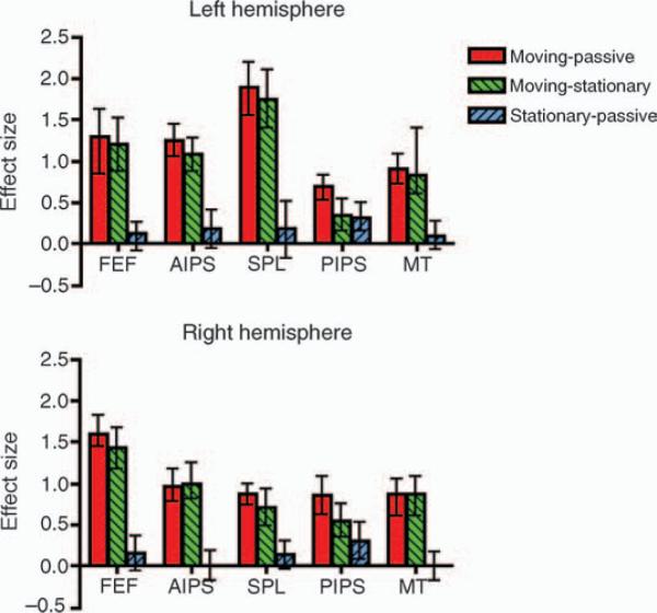
An ROI analysis for each of the 10 brain areas (5 in each hemisphere) for the three possible contrasts. AntIPS = anterior intraparietal sulcus, FEF = frontal eye fields, MT+ = medial temporal complex and SPL = superior parietal lobule. The error bars represent 95% confidence intervals, not corrected for multiple comparisons.
Having identified five brain areas, each activated bilaterally, involved in the MOT task, we wished to determine whether these areas were activated by the act of attending, by the act of tracking, or by both acts. We did this by performing a group region of interest (ROI) analysis on these ten areas. Using the group moving-passive contrast, the 10 ROIs (5 in each hemisphere) were identified (see Materials and methods). For each ROI we report the moving-passive contrast, the moving-stationary contrast and the stationary-passive contrast. The results are shown in Figure 3.
In both the moving and stationary conditions, the observer always attended to the same number of targets. In this sense, the attentional load was the same. However, in the moving condition the observer was also obliged to track the targets. Thus, the moving-stationary contrast (green) isolates the effects of tracking. Figure 3 shows that this contrast was significant in all ten brain areas, suggesting that all these brain areas are involved in tracking. Considering now the stationary-passive contrast (blue), we see that this contrast was significant for only one brain area (PIPS). The stationary condition and the passive condition were identical except that in the former the observer had to attend to two stationary targets. Thus, in our study only PIPS is significantly activated by the act of attending to a stationary object.
To identify the interactions between these brain areas, we used the modified CCD algorithm (Richardson, 1996) to create an undirected graph for each observer that represented the interactions between that observer's brain areas. We then pooled the data from all observers. Performing a Wilcoxon sign rank test on the pooled data revealed no left-right asymmetry between these undirected graphs (n = 20, signed rank = 36, p > 0.21). This justified pooling the left and right hemispherical data to increase accuracy. Since all interhemispheric connections occurred only between the left and right portions of the same brain area, here we show only the connections within a single hemisphere and only those that were found in at least half the observers (Figure 4).
Figure 4.
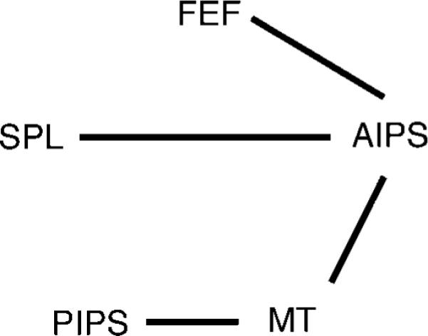
The undirected graph obtained using the modified CCD algorithm. The links denote connections that were found in at least 50% of the observers.
Discussion
The above results show that the FEF, AIPS, SPL, PIPS and MT+ are specifically involved in tracking, each being activated bilaterally. This was found both in the traditional moving-passive contrast and in the more rigorous moving-stationary contrast. As discussed below, while this finding is broadly consistent with previous fMRI studies of MOT, our data suggest that the areas involved in MOT are fewer than previously thought. Using this data, the stationary-passive contrast, and data from previous studies we speculate as to the role these areas may play in MOT. In particular, we consider the relationship between our data and some of the visual short term memory (VSTM) literature, since MOT and VSTM are clearly related (Cavanagh & Alvarez, 2005).
Comparison with other studies
Table 1 shows the results for both this study and the three previous fMRI studies of MOT (Culham et al., 1998, 2001; Jovicich et al., 2001). As these studies used slightly different naming conventions, we adopted just one of them, that of Jovicich et al. (2001). In particular, what Culham et al. (1998) labeled as the precuneus and what Culham et al. (2001) labeled as TrIPS, we label as the transverse parietal sulcus (TranPS) and the posterior IPS (PIPS) respectively.
From Table 1, we see that five brain areas were reported to be activated bilaterally by MOT in all four studies. These areas were the frontal eye fields (FEF), the anterior intraparietal sulcus (AIPS), the superior parietal lobule (SPL), the posterior intraparietal sulcus (PIPS) and the human motion area (MT+). Two areas were identified by the previous three studies but not by the current one. These areas were the supplementary motor area (SMA) and the inferior precentral sulcus. However, whereas Culham et al. (1998) and Jovicich et al. (2001) reported these areas to be active bilaterally, Culham et al. (2001); Figure 3) found activity only on the right side in these areas. The evidence for left SMA activation is further weakened by Culham et al. (1998) finding significant activation in this area in only 2 of their 7 observers. These previous studies either did not perform a group analysis (Culham et al., 1998) or performed only a fixed effects group analysis (Culham et al., 2001; Jovicich et al., 2001), making generalization of their results problematic. By testing more observers and by using a random effects analysis, we were better able to exclude spurious activations. When we performed an ROI analysis using the coordinates for these areas given by Jovicich et al. (2001), we were still unable to find significant activity in either the SMA or the inferior precentral sulcus at the p < 0.05 level (uncorrected for multiple comparisons).
Two areas were reported by only two of the four studies to be activated by MOT: the precuneus and the lateral occipital cortex (Culham et al., 1998; Jovicich et al., 2001). However, this apparent disagreement is probably due to different naming conventions. All studies reported that the area denoted by Culham et al. (1998) as the precuneus to be active. However, whereas Culham et al. (1998) considered this area to be distinct from the superior parietal lobule (SPL), Culham et al. (2001) did not. In this report, we adopted the Culham et al. (2001) definition of SPL. Similarly, the definition of the lateral occipital cortex is also problematic. Whereas Culham et al. (1998) labeled this as a distinct area, Culham et al. (2001) refer to part of this region as the TrIPS (which we call posterior IPS) and the rest of it as MT+.
Six areas have each been reported by only one study. However, one of these reports can be attributed to differences in naming convention: The activity that Culham et al. (1998) attribute to the postcentral sulcus, other studies attribute to the anterior intraparietal sulcus. Another two of the single-area reports can be attributed to differences in experimental paradigms. Jovicich et al. (2001) was the only study to have their observers make motor responses within the scanner. This could explain why theirs was the only study to report activation in the cerebellum and the basal ganglia. The three remaining areas (parieto-insular cortex, Culham et al., 1998; superior frontal sulcus, Culham et al., 2001; anterior cingulate, Jovicich et al., 2001) cannot be attributed to differences in naming conventions or differences in experimental paradigms. As they appear to be unrepeatable, they presumably represent noise.
Possible function of each brain area
In this section, we will consider only the five areas found by all four studies to be activated by MOT: FEF, AIPS, SPL, PIPS and MT+. SPL and FEF are an interesting subset of the network, in that their involvement in tracking depends on the criteria. They are activated more by attending to moving targets than to stationary targets in our data, but their activation is primarily not load dependent (Culham et al., 2001). This is consistent with the idea that the role of SPL and FEF (in MOT) is the generation and suppression of eye movements (Culham et al., 2001). When not required to fixate, observers in MOT experiments typically make saccadic eye movements (Fazl & Mingolla, 2008; Fehd & Seiffert, 2008). Thus, it is likely that although our observers were required to suppress any eye movements, they were still involuntarily planning saccades, which they then had to suppress. SPL is known to be involved in saccade generation (Doricchi et al., 1997) and FEF has been implicated in saccade suppression (Burman & Bruce, 1997; Guitton, Buchtel, & Douglas, 1985; Priori, Bertolasi, Rothwell, Day, & Marsden, 1993).
As MT+ is sensitive to motion (motion localizers were used to identify MT+ in Culham et al., 1998) and is retinotopically organized (e.g. Huk, Dougherty, & Heeger, 2002), it seems likely that its role is to represent the location of moving targets. Activity in MT+ is also known to be modulated by attention (Berman & Colby, 2002), which would explain why MT+ is active when observers attend to moving as opposed to stationary targets.
PIPS is unique among the five areas in that we found that it responds to the act of attending to stationary items. Furthermore, there is strong evidence in Figure 4 for an interaction between PIPS and MT+. If we accept the argument that MT+ represents the locations of objects, then the interaction between PIPS and MT+ is consistent with PIPS indexing which of the objects represented in MT+ are currently being attended. If so, PIPS would be required in order to attend to objects, whether moving or stationary, but may not necessarily be responsible for tracking per se. We discuss the potential role of PIPS more fully in next section.
Finally, along with PIPS, AIPS is also held to be a general purpose attention area (Corbetta et al., 1998; Donner et al., 2000; Wojciulik & Kanwisher, 1999), and previous studies (Culham et al., 2001; Jovicich et al., 2001) reported that its response increased with tracking load. However, AIPS only seems to be brought on line when the targets are moving. This suggests that (in MOT) AIPS is mainly responsible for actively tracking objects, as opposed to simply attending to them. In the undirected graph in Figure 4, AIPS is at the center of the tracking network, underscoring its central importance in tracking. Ignoring interhemispherical connections, we find strong connections between AIPS and three of the other four areas, whereas none of the remaining areas seems to be strongly connected with more than one area besides AIPS.
Finally, note that the modified CCD analysis showed very little evidence for cross-hemispheric interactions, except between the left and right halves of the same brain area. This suggests that the flow of information is mainly contained within a cerebral hemisphere. This predicts that tracking should be easier if the targets are divided across visual hemifields, rather than concentrated in one field or the other, since then both hemispheres can participate in tracking. Precisely this pattern of performance was found in a recent study by Alvarez and Cavanagh (2005).
Relation to VSTM
As Cavanagh and Alvarez (2005) noted, MOT and visual short term memory (VSTM) are tightly linked. The neural underpinnings of MOT and VSTM also appear to overlap. Todd and Marois have noted that neural activity in IPS increases with the number of objects memorized (Todd & Marois, 2004) and that individual differences in IPS activity correlate with individual differences in VSTM capacity (Todd & Marois, 2005). Xu and Chun (2006) have distinguished between the functions of anterior and posterior IPS.1 In their studies, AIPS activity is determined by both the number of objects to be remembered and their complexity. The asymptote in AIPS for simple and complex shapes was predicted by each observer's capacity to remember simple and complex shapes, respectively. Activity in PIPS, in contrast, was related to the number of different locations to be held in memory, asymptoting near four objects, regardless of the objects' complexity. Thus, in Xu and Chun's view, PIPS functions as a spatial index, pointing at the locations of the attended objects, while AIPS represents the features of the remembered object. This is consistent with our findings in MOT, where PIPS seems to represent attended objects even when they are stationary, while AIPS becomes involved when the objects move, perhaps because the computation is then more complex. Thus, AIPS might be involved in updating the locations held in PIPS, or it might represent information about the targets that can be used to track them, such as direction or speed (Fencsik, Klieger, & Horowitz, 2007; Fencsik, Urrea, Place, Wolfe, & Horowitz, 2006).
Conclusions
Our goal in this study was to identify the neural network underlying multiple object tracking. We improved on previous studies in three ways. First, we scanned more observers, and used a random effects analysis. This meant that we could more easily exclude spurious activations. This allowed us to reduce the number of areas relevant to MOT to five areas each activated bilaterally: the frontal eye fields (FEF), the anterior intraparietal sulcus (AIPS), the superior parietal lobule (SPL), the posterior intraparietal sulcus (PIPS) and the human motion area (MT+). Second, we added a condition in which observers attended to stationary targets. This distinguished activity due to attending to targets from activity due to tracking moving targets. We found that all five areas were activated by tracking moving targets, while only PIPS was significantly activated by attending to stationary targets. Finally, we derived an undirected graph of the interactions between these areas using an algorithm modified from computer science (Richardson, 1996). This analysis placed AIPS at the center of the tracking network.
Our data, taken in the context of the relevant literature, suggest that MOT may be achieved by the following architecture: MT+ represents the locations of all the objects in the scene, while PIPS indexes which of the objects are the targets, moving or not. Interactions between these two areas bind indexes to locations. Tracking moving targets also engages AIPS, which represents information about the target in addition to their locations (Xu & Chun, 2006). AIPS in turn communicates with SPL and FEF to suppress eye movements under fixation, and presumably to coordinate eye movements under more naturalistic conditions (Culham et al., 2001). This hypothesis, although consistent with the data in the literature, is necessarily speculative and further research will be needed to test it.
Acknowledgments
PH and ML were supported by EY16187.
Appendix A
The modified CCD algorithm
A worked example
Here we illustrate how the first stage of the CCD algorithm (Richardson, 1996) works with a simple example. For further details and a proof of the validity of this algorithm, the reader is referred to the original source. Suppose Figure A1a represents the true causal relationships between five brain areas: area A projects to areas B and C, which both project to area D, which in turn projects to area E. We start by calculating every possible pairwise correlation. For any pair of brain areas whose time courses are correlated at the 0.05 significance level, Bonferroni corrected for multiple comparisons, we create a link between the pair of brain areas to produce the undirected graph shown in Figure A1b. Thus, each link in this graph represents a statistically significant correlation. However, if a pair of brain areas have correlated activities, this does not prove that they interact because the correlation might be caused by them receiving input from a common source (the common source confound). Thus, some of the link shown in Figure A1b may spurious. The next step is to identify and delete any spurious links.
Figure A1.
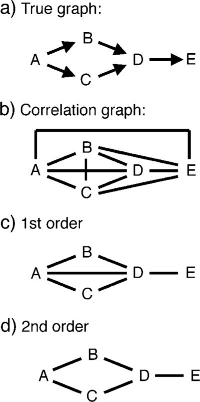
An example of how the modified CCD algorithm works. a) The true directed graph of how the five brain areas interact. b) The graph initially created by the modified CCD algorithm. As all possible pairwise correlations are significant, every brain area is linked directly to every other brain area. c) The result of pruning graph b using first order correlations. d) The result of pruning graph c using second order partial correlations.
We begin by considering each link in Figure A1b in turn to determine if the correlation corresponding to this link was caused by the corresponding pair of brain areas receiving input from just a single common source. We select a node, say node A, and another node that is linked to A, say node E. We then create a set S that contains all the other nodes that are linked to A. In this case, S is {B, C, D}. Set S therefore comprises a set of possible common sources to A and E. We calculate all possible first order partial correlations between A and E that are conditioned on a member of S. In this case, there are three possible partial correlations rAE,B,rAE,C and rAE,D. In this example, since the influence of A and E is mediated by D, we would find rAE,D not to be statistically significant. This would prove that the correlated activity between A and E was caused by these nodes receiving input from D. Thus, we delete the link between A and E as it does not represent a true connection (i.e. it is spurious). This procedure is repeated for all the other nodes that link to A, and then the whole procedure is repeated for each other node in the graph. This results in the undirected graph shown in Figure A1c.
We now consider each link in Figure A1c in turn and consider the possibility that that the link does not represent a true connection but instead the correlation corresponding to this link was caused by the pair of brain areas receiving input simultaneously from two common sources. We test this possibility using second order partial correlations. As before, we start by selecting a node, say node A, and then selected another node that is linked to A, say node D. We then form a set S of the other nodes that are linked to A. In this case, S is {B, C}. We measure all possible second order partial correlations between A and D conditioned on members of set S. In this case, there is only one, rAD,BC. Because this partial correlation is not significant, we know that the correlation between A and D was caused by these two nodes both receiving input from B and C. Thus, the link between A and D does not represent a true connection, so is deleted. This procedure is then repeated for all the other nodes that are linked to A (i.e. B and C) and the whole procedure is then repeated for every other node in the graph. This results in the graph shown in Figure A1d. Since no node is this graph is linked to more than three other nodes, it is not possible that any of these links represent correlations caused the corresponding pair of brain areas receiving input from three or more common sources. Thus, we know that each link represents a true connection, so we are done.
Pseudo code
1) Create an undirected graph G with a node for each brain area. Perform a correlation analysis on the time courses for each possible pair of brain areas. For any correlations that are significant at the 0.05 level, Bonferroni corrected for multiple comparisons, add an link between the corresponding nodes in graph G.
2) Let n represent the order of the partial correlation under consideration. Initialize n to 1.
3) Loop 1: Repeat until all nodes of graph G are linked to less than n + 1 other nodes
Loop 2: Repeat until all nodes of graph G that are linked to at least n + 1 other nodes have been examined
Select a node X of graph G that is linked to at least n + 1 other nodes
Loop 3: Repeat until all nodes connected to X have be examined or node X is no longer linked to at least n + 1 other nodes
i) Select a node Y that is linked to X
ii) Create a set S of the nodes that are linked to X, not including Y
iii) Create a listing of all possible subsets of S, made without replacement, that have cardinality n.
iv) For each subset in turn, measure the partial correlation between X and Y conditioned on the subset. Test at a significance level of 0.05 (not corrected for multiple comparisons, as this was done in step 1). If any of these correlations are not significant, delete the link between X and Y and immediately exit from Loop 3.
End of Loop 3
End of Loop 2
Increment n by 1
End of Loop 1
Footnotes
Commercial relationships: none.
Xu and Chun used the terms “superior” and “inferior” where we use “anterior” and “posterior”; we retain our terminology for consistency.
References
- Allen R, McGeorge P, Pearson DG, Milne AB. Attention and expertise in multiple object tracking. Applied Cognitive Psychology. 2004;18:337–347. [Google Scholar]
- Alvarez GA, Cavanagh P. Independent resources for attentional tracking in the left and right visual hemifields. Psychological Science. 2005;16:637–643. doi: 10.1111/j.1467-9280.2005.01587.x. [DOI] [PubMed] [Google Scholar]
- Alvarez GA, Scholl BJ. How does attention select and track spatially extended objects? New effects of attentional concentration and amplification. Journal Experimental Psychology: General. 2005;134:461–476. doi: 10.1037/0096-3445.134.4.46. [DOI] [PubMed] [Google Scholar]
- Ashburner J, Flandin G, Henson R, Kiebel SJ, Kilner JM, Mattout J, et al. SPM5 Manual. Wellcome Trust Center for Neuroimaging; London: 2007. [Google Scholar]
- Bahrami B. Object property encoding and change blindness in multiple object tracking. Visual Cognition. 2003;10:949–963. [Google Scholar]
- Berman RA, Colby CL. Auditory and visual attention modulate motion processing in area MT+ Cognitive Brain Research. 2002;14:64–74. doi: 10.1016/s0926-6410(02)00061-7. [DOI] [PubMed] [Google Scholar]
- Bonneh YS, Cooperman A, Sagi D. Motion-induced blindness in normal observers. Nature. 2001;411:798–801. doi: 10.1038/35081073. [DOI] [PubMed] [Google Scholar]
- Burman DD, Bruce CJ. Suppression of task-related saccades by electrical stimulation in the primate's frontal eye field. Journal of Neurophysiology. 1997;77:2252–2267. doi: 10.1152/jn.1997.77.5.2252. [DOI] [PubMed] [Google Scholar]
- Carter OL, Burr DC, Pettigrew JD, Wallis GM, Hasler F, Vollenweider FX. Using psilocybin to investigate the relationship between attention, working memory, and the serotonin 1A and 2A receptors. Journal of Cognitive Neuroscience. 2005;17:1497–1508. doi: 10.1162/089892905774597191. [DOI] [PubMed] [Google Scholar]
- Cavanagh P, Alvarez GA. Tracking multiple targets with multifocal attention. Trends in Cognitive Sciences. 2005;9:349–354. doi: 10.1016/j.tics.2005.05.009. [DOI] [PubMed] [Google Scholar]
- Chumbley J, Friston KJ. False discovery rate revisited: FDR and topological inference using Gaussian random fields. Neuroimage. doi: 10.1016/j.neuroimage.2008.05.021. in press. [DOI] [PubMed] [Google Scholar]
- Corbetta M, Akbudak E, Conturo TE, Snyder AZ, Ollinger JM, Drury HA, et al. A common network of functional areas for attention and eye movements. Neuron. 1998;21:761–773. doi: 10.1016/s0896-6273(00)80593-0. [DOI] [PubMed] [Google Scholar]
- Culham JC, Brandt SA, Cavanagh P, Kanwisher NG, Dale AM, Tootell RB. Cortical fMRI activation produced by attentive tracking of moving targets. Journal of Neurophysiology. 1998;80:2657–2670. doi: 10.1152/jn.1998.80.5.2657. [DOI] [PubMed] [Google Scholar]
- Culham JC, Cavanagh P, Kanwisher NG. Attention response functions: Characterizing brain areas using fMRI activation during parametric variations of attentional load. Neuron. 2001;32:737–745. doi: 10.1016/s0896-6273(01)00499-8. [DOI] [PubMed] [Google Scholar]
- Donner T, Kettermann A, Diesch E, Ostendorf F, Villringer A, Brandt SA. Involvement of the human frontal eye field and multiple parietal areas in covert visual selection during conjunction search. European Journal of Neuroscience. 2000;12:3407–3414. doi: 10.1046/j.1460-9568.2000.00223.x. [DOI] [PubMed] [Google Scholar]
- Doricchi F, Perani D, Incoccia C, Grassi F, Cappa SF, Bettinardi V, et al. Neural control of fast-regular saccades and antisaccades: An investigation using positron emission tomography. Experimental Brain Research. 1997;116:50–62. doi: 10.1007/pl00005744. [DOI] [PubMed] [Google Scholar]
- Fazl A, Mingolla E. Predicting eye movement trajectories in a multiple object tracking (MOT) task with free viewing [Abstract] Journal of Vision. 2008;8(6):103, 103a. http://journalofvision.org/8/6/103/, doi:10.1167/8.6.103. [Google Scholar]
- Fehd HM, Seiffert AE. Eye movements during multiple object tracking: Where do participants look? Cognition. 2008;108:201–209. doi: 10.1016/j.cognition.2007.11.008. [DOI] [PMC free article] [PubMed] [Google Scholar]
- Fencsik DE, Klieger SB, Horowitz TS. The role of location and motion information in the tracking and recovery of moving objects. Perception & Psychophysics. 2007;69:567–577. doi: 10.3758/bf03193914. [DOI] [PubMed] [Google Scholar]
- Fencsik DE, Urrea J, Place SS, Wolfe JM, Horowitz TS. Velocity cues improve visual search and multiple object tracking. Visual Cognition. 2006;14:18–21. [Google Scholar]
- Frackowiak RSJ, Friston KJ, Frith C, Dolan R, Price CJ, Zeki S, et al. Human brain function. Academic Press; San Diego, CA: 2003. [Google Scholar]
- Friston KJ, Ashburner J, Poline JB, Frith CD, Heather JD, Frackowiak RSJ. Spatial registration and normalization of images. Human Brain Mapping. 1995;2:165–189. [Google Scholar]
- Genovese CR, Lazar NA, Nichols T. Thresholding of statistical maps in functional neuro-imaging using the false discovery rate. Neuroimage. 2002;15:870–878. doi: 10.1006/nimg.2001.1037. [DOI] [PubMed] [Google Scholar]
- Graf EW, Adams WJ, Lages M. Modulating motion-induced blindness with depth ordering and surface completion. Vision Research. 2002;42:2731–2735. doi: 10.1016/s0042-6989(02)00390-5. [DOI] [PubMed] [Google Scholar]
- Green CS, Bavelier D. Enumeration versus object tracking: Insights from video game players. Cognition. 2006;101:217–245. doi: 10.1016/j.cognition.2005.10.004. [DOI] [PMC free article] [PubMed] [Google Scholar]
- Guitton D, Buchtel HA, Douglas RM. Frontal lobe lesions in man cause difficulties in suppressing reflexive glances and in generating goal-directed saccades. Experimental Brain Research. 1985;58:455–472. doi: 10.1007/BF00235863. [DOI] [PubMed] [Google Scholar]
- Huk AC, Dougherty RF, Heeger DJ. Retinotopy and functional subdivision of human areas MT and MST. Journal of Neuroscience. 2002;22:7195–7205. doi: 10.1523/JNEUROSCI.22-16-07195.2002. [DOI] [PMC free article] [PubMed] [Google Scholar]
- Jovicich J, Peters RJ, Koch C, Braun J, Chang L, Ernst T. Brain areas specific for attentional load in a motion-tracking task. Journal of Cognitive Neuroscience. 2001;13:1048–1058. doi: 10.1162/089892901753294347. [DOI] [PubMed] [Google Scholar]
- Morocz IA, Cosman E, Wells WM, van Gelderen P. Prefrontal networking during mental arithmetic. Annual Meeting of the Organization for Human Brain Mapping.2005. p. 1147. [Google Scholar]
- Morocz IA, van Gelderen P, Shalev R, Spelke ES, Jolesz FA. Temporal unfolding of mental calculation: A 3D PRESTO fMRI study. Annual Meeting of the Organization for Human Brain Mapping.2004. p. 186.95001. [Google Scholar]
- O'Hearn K, Landau B, Hoffman JE. Multiple object tracking in people with Williams syndrome and in normally developing children. Psychological Science. 2005;16:905–912. doi: 10.1111/j.1467-9280.2005.01635.x. [DOI] [PMC free article] [PubMed] [Google Scholar]
- Oldfield RC. The assessment and analysis of handedness: The Edinburgh inventory. Neuropsychologia. 1971;9:97–113. doi: 10.1016/0028-3932(71)90067-4. [DOI] [PubMed] [Google Scholar]
- Paus T. Location and function of the human frontal eye-field: A selective review. Neuropsychologia. 1996;34:475–483. doi: 10.1016/0028-3932(95)00134-4. [DOI] [PubMed] [Google Scholar]
- Petit L, Clark VP, Ingeholm J, Haxby JV. Dissociation of saccade-related and pursuit-related activation in human frontal eye fields as revealed by fMRI. Journal of Neurophysiology. 1997;77:3386–3390. doi: 10.1152/jn.1997.77.6.3386. [DOI] [PubMed] [Google Scholar]
- Priori A, Bertolasi L, Rothwell JC, Day BL, Marsden CD. Some saccadic eye movements can be delayed by transcranial magnetic stimulation of the cerebral cortex in man. Brain. 1993;116:355–367. doi: 10.1093/brain/116.2.355. [DOI] [PubMed] [Google Scholar]
- Pylyshyn ZW, Storm RW. Tracking multiple independent targets: Evidence for a parallel tracking mechanism. Spatial Vision. 1988;3:179–197. doi: 10.1163/156856888x00122. [DOI] [PubMed] [Google Scholar]
- Richardson TS. A discovery algorithm for directed cyclic graphs. Morgan Kaufmann; San Francisco, CA: 1996. [Google Scholar]
- Scholl BJ. What have we learned about attention from multiple object tracking (and vice versa) In: Dedrick D, Trick L, editors. Computation, cognition, and pylyshyn. MIT Press; Cambridge, MA: in press. [Google Scholar]
- Scholl BJ, Pylyshyn ZW, Feldman J. What is a visual object? Evidence from target-merging in multiple-object tracking. Cognition. 2001;80:159–177. doi: 10.1016/s0010-0277(00)00157-8. [DOI] [PubMed] [Google Scholar]
- Sears CR, Pylyshyn ZW. Multiple object tracking and attentional processing. Canadian Journal of Experimental Psychology. 2000;54:1–14. doi: 10.1037/h0087326. [DOI] [PubMed] [Google Scholar]
- Todd JJ, Marois R. Capacity limit of visual short-term memory in human posterior parietal cortex. Nature. 2004;428:751–754. doi: 10.1038/nature02466. [DOI] [PubMed] [Google Scholar]
- Todd JJ, Marois R. Posterior parietal cortex activity predicts individual differences in visual short-term memory capacity. Cognitive Affective Behavioral Neuroscience. 2005;5:144–155. doi: 10.3758/cabn.5.2.144. [DOI] [PubMed] [Google Scholar]
- Trick LM, Jaspers-Fayer F, Sethi N. Multiple-object tracking in children: The “Catch the Spies” task. Cognitive Development. 2005;20:373–387. [Google Scholar]
- VanMarle K, Scholl BJ. Attentive tracking of objects versus substances. Psychological Science. 2003;14:498–504. doi: 10.1111/1467-9280.03451. [DOI] [PubMed] [Google Scholar]
- Vul E, Kanwisher M. Begging the question: The non-independence error in fMRI data analysis. In: Hanson S, Bunzl M, editors. Foundational issues for human brain mapping. MIT Press; in press. [Google Scholar]
- Wojciulik E, Kanwisher N. The generality of parietal involvement in visual attention. Neuron. 1999;23:747–764. doi: 10.1016/s0896-6273(01)80033-7. [DOI] [PubMed] [Google Scholar]
- Xu Y, Chun MM. Dissociable neural mechanisms supporting visual short-term memory for objects. Nature. 2006;440:91–95. doi: 10.1038/nature04262. [DOI] [PubMed] [Google Scholar]