Image-based models of cardiac structure with applications in arrhythmia and defibrillation studies

Abstract

The objective of this article is to present a set of methods for constructing realistic computational models of cardiac structure from high-resolution structural and diffusion tensor magnetic resonance images and to demonstrate the applicability of the models in simulation studies. The structural image is segmented to identify various regions such as normal myocardium, ventricles, and infarct. A finite element mesh is generated from the processed structural data, and fiber orientations are assigned to the elements. The Purkinje system, when visible, is modeled using linear elements that interconnect a set of manually identified points. The methods were applied to construct 2 different models; and 2 simulation studies, which demonstrate the applicability of the models in the analysis of arrhythmia and defibrillation, were performed. The models represent cardiac structure with unprecedented detail for simulation studies.

Introduction

The primary cumulative goal of all cardiac research is a comprehensive understanding of the structure and function of the heart in health and disease. A key to achieving this goal is the integration of information obtained at various levels, from ion channels and calcium cycling to activation maps and regional strain distributions. Computational modeling provides a powerful tool to address this challenge and is thus becoming essential for the complete understanding of the heart. Computational approaches require finite element representations (or models) of the geometry and fiber architecture of the cardiac tissue.¹ The cardiac architecture must be accurately acquired to construct realistic models. Recent advances in magnetic resonance (MR) imaging technologies have facilitated the acquisition of geometry and tissue architecture of the heart at very high spatial resolution. Modern anatomical MR scanners can image the cardiac histoanatomy of small experimental animals, such as rabbit, with an isotropic resolution in the order of 10⁻⁵ m.² Advanced diffusion tensor (DT) MR equipments can measure the diffusivity of water in the tissue with a resolution in the order of 10⁻⁴ m.³ The primary eigenvectors of the DTs have been shown to be aligned with the prevailing cardiomyocyte orientations, commonly referred to as “fiber orientations.” Evidence also suggests that the secondary and tertiary eigenvectors are oriented normally to the main cell axes, in the myocardial laminar plane and perpendicular to it, respectively.

The objective of this article is twofold. First, we present a set of generic methods that we have developed for constructing detailed computational models of the heart from high-resolution structural and DTMR images. Second, we demonstrate the application of these models in the study of arrhythmia and defibrillation. The models that we present contain unprecedented structural detail, opening enhanced opportunities for modeling cardiac function. In the following, Section 2 presents the methods for generating whole-heart models, Section 3 presents the reconstructed whole-heart models, Section 4 describes the reconstruction of the Purkinje network, Section 5 reports results of electrophysiologic simulation studies, demonstrating the utility of image-based modeling in arrhythmia and defibrillation research, and Section 6 concludes the article.

Methodology for image-based whole-heart model generation

Segmentation of the structural image

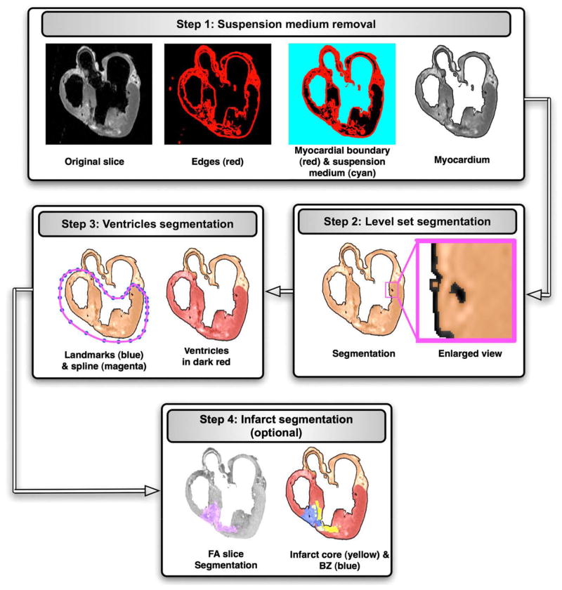
To generate image-based models of the heart, it is necessary to classify (or segment) the voxels in the structural MR image into different groups, such as normal tissue, diseased tissue (or infarct), background, and so on. Segmentation of high-resolution cardiac images is a very challenging task because of the complex geometry and topology of the myocardium, measurement noise, blurred object boundaries in the images, and the overlap of image intensities between different voxel groups. After extensive experimentation with various existing segmentation techniques such as edge detection, deformable models, region growing, level set methods, k-means clustering, and so on,⁴ we developed a processing pipeline for the segmentation of the structural MR image as illustrated in Fig. 1. The figure shows the results as an example image slice is processed through the steps 1 to 4 in the pipeline. Step 1 in the figure shows the original example slice. The steps of the pipeline are explained in detail below.

Fig. 1.

The application of the segmentation pipeline to an example image slice. The sequence of rectangular blocks illustrates the results as an example image slice is processed through the steps 1 to 4 in the pipeline.

Suspension medium removal

In the first step of our segmentation pipeline, the structural MR image is processed to label and “remove” the voxels corresponding to the cavity content, and the medium in which the heart was suspended during the image acquisition. A combination of edge detection, region growing, and manual editing is used in this step. The edge detection is performed in each slice of the image, by first computing the intensity variance of the 2-dimensional (2D) local neighborhood of each voxel in the slice and then by selecting voxels with a variance above a certain threshold. Step 1 in Fig. 1 shows the edges for the example slice. The collection of image slices after the edge detection forms the edge image, a 3-dimensional (3D) map of the 2D edges.

From the edge image, the myocardial boundary of the whole heart is extracted using a 3D region growing algorithm. This algorithm, when initialized with a user defined voxel, identifies a voxel set such that the set forms a connected structure, which includes the user defined voxel; the members of the set have the same image intensity. Next, from the image that represents the myocardial boundary, voxels that correspond to the suspension and cavity medium are extracted using the region growing algorithm. Finally, the suspension medium is removed from the original structural MR image by assigning the background intensity to all voxels that correspond to the medium. Step 1 in Fig. 1 shows the myocardial boundary, suspension medium, and myocardium for the example slice. The collection of image slices after the removal of the suspension medium forms a 3D image of the myocardium.

Level set segmentation

In the next step, a level set method is applied to the image of the myocardium, to separate the larger coronary arteries and interlaminar clefts, as well as to refine the myocardial boundary extracted during the previous steps. Level set methods have the inherent capability to implicitly track complex topologies. This characteristic makes them highly suitable for the delineation of the complex coronary artery network and interlaminar clefts. In the level set methods, the segmentation is achieved through the evolution of a surface Γ, which is implicitly represented as the zero level set of a time-dependent 3D function Φ(x, y, z, t), i.e. Γ(t) = {x, y, z|Φ(x, y, z, t) = 0}, where x, y, z are the Cartesian coordinates, and t is the time. The evolution of Φ is formulated as a partial differential equation, which contains terms for advancing the surface based on image intensities, smoothening the surface, and attracting the surface to the edges in the image. For detailed information on the level set segmentation, the reader is referred to reference 5. Step 2 in Fig. 1 illustrates the level set segmentation for the example slice. It must be noted that it is necessary to remove the suspension medium before the level set segmentation because the surface may otherwise evolve into the medium in image regions where the boundary between myocardium and medium is blurred.

Segmentation of ventricles

In the third step of our model generation pipeline, segmentation of the ventricular myocardium is performed to account for the presence of an insulating layer of connective tissue between the atria and the ventricles (annulus fibrosus), as well as to assign different electrophysiologic properties (atrial vs ventricular) to the tissue on either side of this boundary. To perform this step, in each slice, the ventricular portion of the tissue is labeled by fitting a closed spline curve through landmark points placed around the ventricles and along the atrioventricular (AV) border. All voxels that belong to tissue inside the curve are marked as ventricular. Step 3 in Fig. 1 shows the landmarks, spline, and ventricular myocardium for the example slice. The identification of landmark points is performed manually for a number of slices that are evenly distributed in the image. The manual placement of the landmarks is guided by the elevated voxel intensity of the dense tissue along the AV border and the location of AV valves. The landmarks for the remaining slices are obtained by linearly interpolating the manually identified points.

Mathematically, let s₁, s₂, s₃,…,s_n denote the sequence of slices in the image, and let s_i1, s_i2, s_i3,…, s_im denote the slices for which the landmarks are identified manually, where i₁ < i₂ < i₃ < … < i_m. The number of landmarks is the same in every slice. Let p denote the number of landmarks, and let l₁, l₂, l₃,…,l_pdenote the landmarks. Note that a landmark in one slice is denoted by the same index as the corresponding landmark in any other slice. If ( $x_j^{i_a},y_j^{i_a}$) and ( $x_j^{i_{a+1}},y_j^{i_{a+1}}$) are the coordinate pairs of landmark l_j on slices s_ia and s_{ia + 1} respectively, then the coordinates of l_j on slices s_k, i_a < k < i_{a + 1} are given by

$$\{\begin{array}{l}{x}_j^k=x_j^{i_a}+\frac{(j_k-i_a)}{(i_{a+1}-i_a)}\left(x_j^{i_{a+1}}-x_j^{i_a}\right),\hfill \\ y_j^k=y_j^{i_a}+\frac{(j_k-i_a)}{(i_{a+1}-i_a)}\left(y_j^{i_{a+1}}-y_j^{i_a}\right)\hfill \end{array}$$ (1)

Infarct segmentation

After the delineation of the ventricles, any infarct tissue present is labeled using a combination of level set segmentation of the fractional anisotropy (FA) image, intensity thresholding of the anatomical image. In this procedure, the DTMR image is interpolated to the resolution of the structural MR image if the resolution of the latter is higher. The interpolation of the DTMR image is performed by first linearly interpolating the diffusion-weighted images to the desired resolution and then recalculating the local DTs using existing methods.⁶ From the interpolated DTMR image, the FA image is generated by computing the FA of the DT at each voxel.⁷ The FA is a measure of the directional diffusivity of water, and its values range from 0 to 1. A value of 0 indicates perfectly isotropic diffusion, and 1 indicates perfectly anisotropic diffusion. The infarct region is characterized by lower anisotropy, and therefore lower FA values, compared to the healthy myocardium⁸ because of the myocardial disorganization in the infarct. Based on this difference in FA values, the infarct region is separated from the normal myocardium by applying a level set segmentation to the 3D FA image. Step 4 in Fig. 1 shows the segmentation of the FA image slice that corresponds to the example slice. Next, the infarct region is subdivided into 2 areas, a core, which is assumed to contain inexcitable scar tissue, and a border zone, which is assumed to contain excitable but pathologically remodeled tissue, by thresholding the structural MR image based on the intensity values of the voxels. The core has high or low intensity, whereas the border zone has medium intensity.^9,10 Step 4 in Fig. 1 illustrates the final segmentation of the example slice. Once any infarct areas present are identified, segmentation of the structural MR image is complete.

Mesh generation

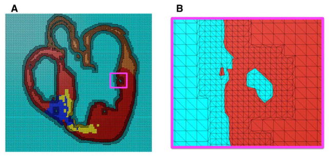
Next, a finite element mesh is generated from the segmented structural MR image using Tarantula, a commercial software (http://www.meshing.at/Spiderhome/Tarantula.html). Details regarding the mesh generation methodology can be found in a recent article.¹¹ The software is very robust; produces boundary-fitted, locally refined, smooth conformal meshes; and allows the user to select the desired resolution in various regions. The software automatically assigns region identifiers to the elements based on the segmentation, thereby differentiating the elements that belong to the infarct regions, the ventricles, or the rest of the tissue. Fig. 2A shows a mesh generated for the segmented slice shown in Fig. 1. Fig. 2B presents a small region of the mesh in detail. As the figure illustrates, the interior tissue volume is meshed at low resolution, whereas the interface between tissue and nontissue is refined by a factor of about 2. This local adaptation of the resolution significantly reduces the number of elements in the mesh without compromising the geometric detail.

Fig. 2.

Mesh generation: (A) mesh corresponding to the segmented image slice shown in Fig. 1; (B) enlarged view of the small region enclosed by the magenta box in A.

Fiber mapping

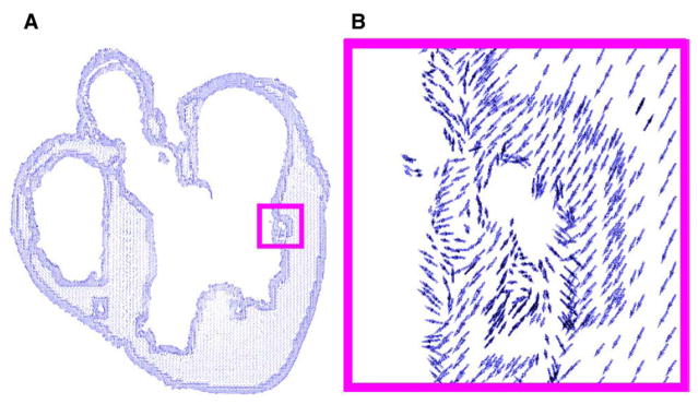
In the final step of the model generation pipeline, fiber orientations are mapped onto the anatomical mesh by interpolating the primary diffusion vectors on the centroids of the elements. First, a reference vector field is constructed by computing the primary eigenvector of each tensor in the previously interpolated DTMR image. This vector field is in the same coordinate system as the finite element mesh. The fiber orientation assigned to an element in the mesh is the direction of that vector in the reference field nearest to the centroid of the element. Fig. 3A shows the derived fiber orientations, mapped to the mesh shown in Fig. 2A. Fig. 3B shows a small region in more detail.

Fig. 3.

Assignment of fiber orientations: (A) 2D projection of orientations assigned to the mesh shown in Fig. 2A; (B) enlarged view of the small region enclosed by the magenta box in A.

Data sets and whole-heart models

Models were generated from MR data sets of a normal rabbit heart and a rabbit heart with cardiac infarction. For the infarcted heart, both structural MR and DTMR images were acquired, at resolutions of 61 × 61 × 60 and 122 × 122 × 500 μm³, respectively. The infarct was 4 weeks old and induced by occlusion of the lateral division of the coronary artery.¹² For the normal heart, only the structural MR image was acquired, at a very high resolution of 26.5 × 26.5 × 24.5 μm³. These data sets have been used in a previous studies, where data acquisition techniques have been described.^2,13

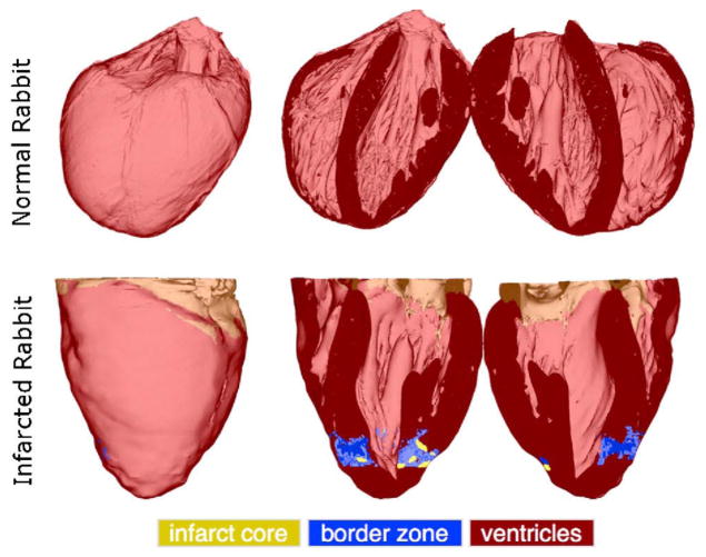
Fig. 4 visualizes the generated whole-heart models. In each row, the first column shows the anterior view of the entire organ model, and the second and third columns show the model split open along the horizontal long axis view plane. Ventricles, infarct cores, and border zones are shown in dark red, yellow, and blue, respectively. The developed methods have reconstructed the overall geometries of the hearts. In the normal rabbit heart data set, the atria had collapsed in the process of data acquisition, which necessitated the removal of all tissue that does not belong to the ventricular myocardium. The normal rabbit model consisted of approximately 31 million elements, and the infarcted model consisted of 1 million elements. The average edge lengths in the normal and infarcted models were 50 and 230 μm, respectively.

Fig. 4.

The models of normal and infarcted rabbit hearts. In each row, the first column shows the anterior view of the entire model, and the second and third columns show the model split in half along a horizontal long-axis view plane.

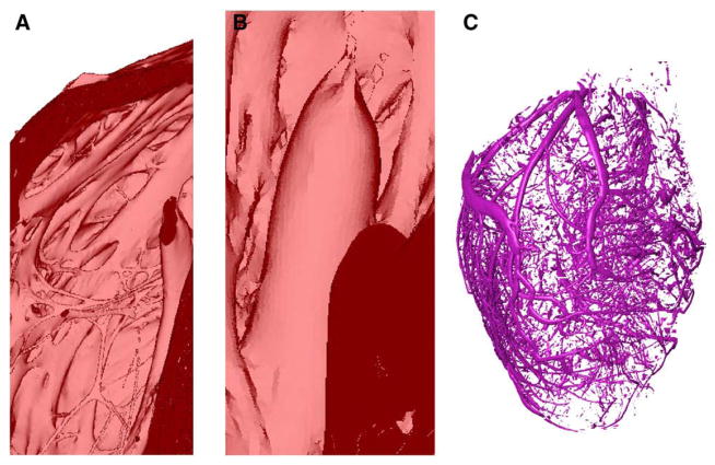
Fig. 5A shows an enlarged view of the muscular trabeculations in the basal region of the right ventricular (RV) chamber in the normal rabbit model. Fig. 5B presents a papillary muscle that is attached to the mitral valve in the infarcted rabbit model. Fig. 5C shows the extracted coronary vessels and interlaminar clefts in the normal rabbit model. Note that the vessels and clefts are separated from the rest of the myocardium during the level set segmentation. The reconstruction of the papillary muscles and of the complex network of trabeculations, arteries, and interlaminar clefts illustrate the high resolution of the structural detail that can be obtained using the methods developed here.

Fig. 5.

Demonstration of the structural detail that can be obtained using our processing pipeline: (A) the endocardial trabeculations in the basal region of the RV in the normal rabbit model; (B) a papillary muscle that is attached to the mitral valve of the infarcted rabbit model; (C) blood vessels and interlaminar clefts in the normal rabbit model.

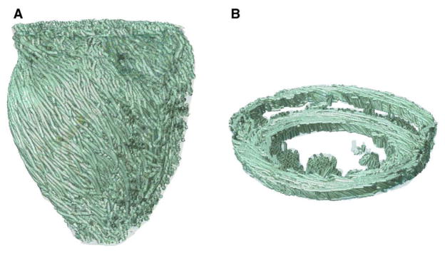
Visualization of the 3D arrangement of fiber orientations in the heart is a challenging problem. A common solution is to use the so-called streamlining method.¹⁴ In this method, fiber orientation is displayed as a track, which is traced by moving a particle according to the velocity field defined by the primary diffusion vectors. To obtain a smooth visualization, it is important to remove measurement noise by filtering the velocity field. To do so, we used a locally regularizing filter called the Perona-Malik Nonlinear Anisotropic filter.¹⁵ Fig. 6 displays the primary eigenvector tracks for the infarcted rabbit model. A visual comparison of the tracks with existing anatomical data^16,17 verifies the qualitative correlation of the fiber orientations in these models.

Fig. 6.

Visualization of fiber tracks, indicative of regionally prevailing cell orientation, in the infarcted rabbit model. (A) Epicardial view of tracks in the entire model; (B) tracks in a slab of tissue between 2 short-axis planes.

Purkinje system modeling

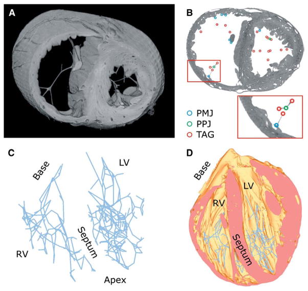
We have developed a methodology for reconstructing the Purkinje System (PS) from a high-resolution structural MR image and a finite element mesh representing the normal rabbit ventricles. Explicit reconstruction of the PS incorporates additional structural detail into the whole-heart model and allows the user to assign distinct electrophysiologic properties to the PS. For each slice in the image, branching points within the free-running PS (Purkinje-Purkinje junctions, PPJs) and points where the PS entered the myocardium (Purkinje-myocardial junctions, PMJs) are identified by visual inspection and spatial coordinates of these points are recorded. To construct the model of the free-running PS, the PMJ and PPJ points are mapped onto the closest vertices in the finite element mesh and connected using linear elements, with intermediate points or tags inserted in segments that deviated noticeably from straight lines. Although this eliminated the elegant curvature of the physical system, the preservation of junctions and bifurcations ensures that the resulting model is an excellent approximation from an electrophysiologic perspective.

The above methodology was applied to the high-resolution structural MR image of the normal rabbit heart and the corresponding finite element mesh. Fig. 7 shows the results. Fig. 7A shows a slab of the mesh that lies between 2 short-axis planes. Fig. 7B illustrates the PMJs, PPJs, and tags on a short-axis slice of the image. The inset in Fig. 7B displays the enlarged view of the small region enclosed in the red box. In the RV, there were 70 PPJs and 71 PMJs, with 49 of PMJs being found on the free wall, 10 on papillary muscles, and 12 on the septum. In the larger left ventricle, 138 PPJs and 99 PMJs were found, with 61, 24, and 14 PMJs, respectively, situated at the sites reported for the RV. Fig. 7C shows the reconstructed model of the entire PS, and Fig. 7D shows the PS overlaid on the mesh.

Fig. 7.

Reconstructing the PS: (A) a slab of the mesh that lies between 2 short-axis planes; (B) the PMJs, PPJs, and tags on a short-axis slice of the image. The inset displays the enlarged view of the small region enclosed in the red box; (C) the reconstructed PS; (D) the PS overlaid on the mesh.

Simulation examples of defibrillation and arrhythmia in the generated models

In this section, we present 2 different electrophysiologic simulation examples using each of the 2 models presented in Section 3. The first study uses the infarcted rabbit model to investigate the influence of the infarct core on the formation of virtual electrodes at defibrillation shock-end. In the second study, the RV free wall extracted from the high-resolution normal rabbit model is subject to pacing stimuli to examine reentrant waves. These studies use cardiac models with unprecedented structural detail and demonstrate the utility of image-based modeling in arrhythmia and defibrillation research. The studies have not been published previously.

Shock-end virtual electrode polarization in infarcted rabbit model

The infarcted rabbit model was used for a bidomain simulation study of virtual electrode polarization (VEP) formation at shock-end. We hypothesized that the infarct core would influence the formation of VEPs in the area of the core. Different VEP patterns at shock-end can ultimately lead to different post-shock propagating behavior and, in the case of defibrillation shocks, to different shock outcomes. For example, positive VEPs can lead to repolarization in regions where tissue is excitable (termed make excitation because it occurs at shock onset). Negative VEP, on the other hand, can deexcite action potentials, creating post-shock excitable gaps. Close spatial proximity of such deexcited regions with positive VEPs can result in “break” excitation at shock-end.¹⁸

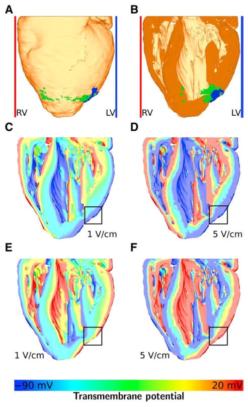
The left ventricular shocks were defined to occur when a plate electrode next to the left ventricle (blue bar in Fig. 8A and B) was used as the cathode and a plate electrode next to the RV (red bar in Fig. 8A and B) was used as ground. For RV shocks, the opposite arrangement was used. Left and RV shocks of 1 and 5 V/cm strength and of 5-millisecond duration each were applied with a coupling interval (the time between the last pacing stimulus and shock onset) of 160 milliseconds after apical pacing.

Fig. 8.

Simulations of the infarcted rabbit model showing the effect of the infarct core on shock-end virtual electrode polarizations. A, The whole heart model with infarct core (blue), border zone (green), and the plate electrodes. B, The heart cut in half at a coronal plane. C, Transmembrane potential at shock-end of a 1 V/cm left ventricular shock. D, Transmembrane potential at shock-end of a 5 V/cm left ventricular shock. E, Transmembrane potential at shock-end of a 1 V/cm right ventricular shock. F, Transmembrane potential at shock-end of a 5 V/cm right ventricular shock. The color bar for C through F is shown in the bottom panel. Transmembrane potentials of −90 mV or less are colored as −90 mV, and potentials of 20 mV or more are colored as 20 mV.

The Mahajan-Shiferaw rabbit ventricular ionic model was used to simulate the action potential.¹⁹ This ionic model is capable of representing the properties of fast ventricular action potential of the rabbit and therefore it is a model well suited for the study of arrhythmia and arrhythmia therapy. To account for the behavior of ventricular myocytes after applied shocks,^18,20 and to maintain stability during the drastic changes in transmembrane potentials occurring during shocks,²¹ the ionic model was modified by adding electroporation and I_a current. It was assumed that I_a is part of the K⁺ flow through the L-type Ca²⁺ channel I_Ca,L.¹⁸ The infarct core was modeled as passive tissue with a resting potential of −80 mV.²² The intracellular and extracellular longitudinal conductivities were both set to 0.295 S/m. The transverse conductivities were set to 0.046 and 0.184 S/m for the intracellular and extracellular spaces, respectively.²³ For the infarct core, normal conductivity values were reduced by half.²⁴

Fig. 8A shows the whole heart model in an anterior-posterior view (ie, the heart is viewed from the front, the RV can be seen on the left, the left ventricle can be seen on the right). The border zone is marked in green, and the infarct core is marked in blue. Fig. 8B shows the posterior part of the heart after the model was cut in half along a coronal plane. Fig. 8C to F display the simulation results overlaid on the coronal cut. Fig. 8C shows the distribution of transmembrane potential V_m at shock-end of a 1 V/cm left ventricular shock, Fig. 8D shows V_m at shock-end of a 5 V/cm left ventricular shock, Fig. 8E shows V_m at shock-end of a 1 V/cm RV shock, and Fig. 8F shows V_m at shock-end of a 5 V/cm RV shock. Note that both the border zone was modeled as infarct core, resulting in a larger core, and no border zone. The region of the infarct core is approximately marked by the black squares in Fig. 8C to F. The color bar for transmembrane potentials shown in the bottom panel applies to Fig. 8C to F.

The results show that, at shock-end, VEP is present in all transmural areas of the heart, with virtual cathodes facing the ground electrodes and virtual anodes facing the cathodes (plate electrodes). Also, with higher shock strengths, the gradients in transmembrane potential between virtual cathodes and anodes become steeper and virtual anodes and cathodes lie closer together spatially. In Fig. 8C and E (1 V/cm shocks), large areas of tissue lie between positive (red) and negative (blue) VEPs. In Fig. 8D and F (5 V/cm shocks), on the other hand, positive and negative VEPs lie closer together. Close to the site of the infarction (see Fig. 8B), the virtual anode (blue color coding) is more pronounced than in other parts of the tissue. For 1 V/cm shocks (Fig. 8C and E), no virtual cathode (red color coding) is present in the area of the infarction.

This more prevalent virtual anode, in conjunction with a less prevalent virtual cathode, leads to an increased excitable gap in the area of the infarction. Defibrillation shocks are successful if they abolish fibrillatory activity and do not induce new fibrillation wave fronts. In terms of VEPs, defibrillation shocks are successful if make and break excitations travel through shock-induced excitable gaps before the rest of the ventricles becomes excitable again.¹⁸ Therefore, a larger excitable gap, as was observed in the area of the infarction in this study, can compromise shock outcome. In this study, an image-based cardiac model with unprecedented structural detail has been used for the first time to demonstrate the formation of VEPs.

Reentry in the RV free wall

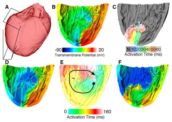
A geometrical mesh of the RV free wall was extracted from the model of the normal rabbit heart shown in Fig. 4. Fig. 9A illustrates the extracted RV wall. Because DTMR data were not available for the normal rabbit case, fiber orientations were assigned to the elements using a recently developed algorithm.²⁵ This algorithm has been found to match DTMR-derived fiber orientations with an accuracy of 95%. The resultant RV free wall model consisted of approximately 15 million elements.

Fig. 9.

Initiation of an apical wave reentry in the rabbit right ventricular free wall. A, Surface of rabbit ventricles with right ventricular wall boxed in. B, Voltage map of second reentrant beat initiated by premature line stimulus in the wake of a propagating wave. C and D, Activation and voltage maps, respectively, of third and final pacing stimulus and subsequent wave propagation. E and F, Activation and voltage maps, respectively, of a reentrant beat after initiation as shown in C and D. The color bar in B applies to D and F also.

The tissue active response was modeled again using the rabbit ventricular ionic model.¹⁹ Pacing stimuli were applied from the apex (bottom of Fig. 9B–F), beginning at a basic cycle length of 210 milliseconds and decreasing to a minimum of 168 milliseconds. After 8 pulses were applied at a cycle length of 168 milliseconds, a large stimulus was applied to the lower right quarter of the model in the refractory tail of the last paced wave. This initiated one beat of reentry (ending as shown in Fig. 9B). Three line stimuli were applied in the excitable gap of this reentrant wave (as shown in Fig. 9C–D) to reinitiate reentry until the tissue was able to sustain a reentrant wave unassisted. In Fig. 9D, the voltage map was taken at time of stimulus application, while the activation map shows from then through 60 milliseconds later. Colored isochrones in Fig. 9C represent 10 milliseconds of propagation per color as shown in the scale. An example of one beat of such reentry is shown in Fig. 9E to F. In Fig. 9F, voltage map was taken in the middle of the period shown in Fig. 9E. The black arrow in Fig. 9E indicates approximate direction of propagation starting at the circle and ending near the arrow. Colored isochrones in Fig. 9E represent 10 milliseconds of propagation per color, with values indicated by the scale. The reentrant pathway is shown in Fig. 9E, whereas a snapshot of transmembrane potential during the same reentrant beat is shown in Fig. 9F. Reentry was sustained for at least 3 seconds.

During reentry, no consistent reentrant pathway was observed. Rather, on each rotation, the wave meandered through the various endocardial structures and the bulk tissue in the ventricular wall. The long, thin network of strands was occasionally responsible for transmitting activation to a region at rest, although typically the activation wave front moved through the bulk of the wall itself. Qualitatively, the pattern of wave front propagation was reminiscent of polymorphic rather than of monomorphic ventricular tachycardia. The simulation study enables us for the first time to examine the role of endocardial structures such as trabeculations in initiation and maintenance of reentry.

Concluding remarks

This report presents a set of generic methods for reconstructing high-resolution 3D heart models from structural MR and DTMR images and demonstrates the utility of these models in the study of arrhythmia and defibrillation. The models presented in this article offer hitherto unavailable structural detail, heralding enhanced opportunities for modeling cardiac electrophysiology. In particular, our models contain fine details of the cardiac geometry such as endocardial trabeculations and the PS, and incorporate atrial and ventricular fiber data acquired at resolutions in the order of 10⁻⁴ m. The simulation studies presented here are the first to demonstrate that highly detailed image-based cardiac models can be used in the study of arrhythmia and defibrillation.

References

- 1.Hunter PJ, Pullan AJ, Smaill BH. Modeling total heart function. Annu Rev Biomed Eng. 2003;5:147. doi: 10.1146/annurev.bioeng.5.040202.121537. [DOI] [PubMed] [Google Scholar]
- 2.Burton RAB, Plank G, Schneider JE, et al. Three-dimensional models of individual cardiac histoanatomy: tools and challenges. Ann N Y Acad Sci. 2006;1080:301. doi: 10.1196/annals.1380.023. [DOI] [PMC free article] [PubMed] [Google Scholar]
- 3.Helm PA, Younes L, Beg MF, et al. Evidence of structural remodeling in the dyssynchronous failing heart. Circ Res. 2006;98:125. doi: 10.1161/01.RES.0000199396.30688.eb. [DOI] [PubMed] [Google Scholar]
- 4.Suri JS, Kamaledin SS, Singh S. Advanced algorithmic approaches to medical image segmentation: state of the art applications in cardiology, neurology, mammography, and pathology. London: Springer-Verlag; 2002. [Google Scholar]
- 5.Ibanez L, Schroeder W, Ng L, Cates J. The Itk software guide: the insight segmentation and registration toolkit. Clifton Park, New York: Kitware Inc; 2003. [Google Scholar]
- 6.Chen J, Liu W, Zhang H, et al. Regional ventricular wall thickening reflects changes in cardiac fiber and sheet structure during contraction: quantification with diffusion tensor MRI. Am J Physiol Heart Circ Physiol. 2005;289:H1898. doi: 10.1152/ajpheart.00041.2005. [DOI] [PubMed] [Google Scholar]
- 7.Basser PJ, Pierpaoli C. Microstructural and physiological features of tissues elucidated by quantitative-diffusion-tensor MRI. J Magn Reson. 1996;111:209. doi: 10.1006/jmrb.1996.0086. [DOI] [PubMed] [Google Scholar]
- 8.Chen J, Song S-K, Liu W, et al. Remodeling of cardiac fiber structure after infarction in rats quantified with diffusion tensor MRI. Am J Physiol Heart Circ Physiol. 2003;285:H946. doi: 10.1152/ajpheart.00889.2002. [DOI] [PubMed] [Google Scholar]
- 9.Schmidt A, Azevedo CF, Cheng A, et al. Infarct tissue heterogeneity by magnetic resonance imaging identifies enhanced cardiac arrhythmia susceptibility in patients with left ventricular dysfunction. Circulation. 2007;115:2006. doi: 10.1161/CIRCULATIONAHA.106.653568. [DOI] [PMC free article] [PubMed] [Google Scholar]
- 10.Wu M-T, Tseng W-YI, Su M-YM, et al. Diffusion tensor magnetic resonance imaging mapping the fiber architecture remodeling in human myocardium after infarction: correlation with viability and wall motion. Circulation. 2006;114:1036. doi: 10.1161/CIRCULATIONAHA.105.545863. [DOI] [PubMed] [Google Scholar]
- 11.Prassl AJ, Kickinger F, Ahammer H, et al. Automatically generated, anatomically accurate meshes for cardiac electrophysiology problems. IEEE Trans Biomed Eng. 2009 doi: 10.1109/TBME.2009.2014243. [in revision] [DOI] [PMC free article] [PubMed] [Google Scholar]
- 12.Kim SC, Vasanji A, Efimov I, Cheng Y. Spatial distribution and extent of electroporation by strong internal shock in intact structurally normal and chronically infarcted rabbit hearts. J Cardiovasc Electrophysiol. 2009 doi: 10.1111/j.1540-8167.2008.01201.x. [in press] [DOI] [PMC free article] [PubMed] [Google Scholar]
- 13.Vadakkumpadan F, Arevalo H, Prassl AJ, et al. Image-based models of cardiac structure in health and disease. IEEE Trans Med Imaging. 2009 doi: 10.1002/wsbm.76. [under review] [DOI] [PMC free article] [PubMed] [Google Scholar]
- 14.Rohmer D, Sitek A, Gullberg GT. Reconstruction and visualization of fiber and laminar structure in the normal human heart from ex vivo diffusion tensor magnetic resonance imaging (DTMRI) data. Invest Radiol. 2007;42:777. doi: 10.1097/RLI.0b013e3181238330. [DOI] [PubMed] [Google Scholar]
- 15.Perona P, Malik J. Scale-Space and edge detection using anisotropic diffusion. IEEE Trans Pattern Anal Mach Intell. 1990;12:629. [Google Scholar]
- 16.Helm P, Beg MF, Miller M, Winslow R. Measuring and mapping cardiac fiber and laminar architecture using diffusion tensor MR imaging. Ann N Y Acad Sci. 2005;1047:296. doi: 10.1196/annals.1341.026. [DOI] [PubMed] [Google Scholar]
- 17.Streeter DDJ, Spotnitz HM, Patel DP, Ross JJ, Sonnenblick EH. Fiber orientation in the canine left ventricle during diastole and systole. Circ Res. 1969;24:339. doi: 10.1161/01.res.24.3.339. [DOI] [PubMed] [Google Scholar]
- 18.Trayanova N. Defibrillation of the heart: insights into mechanisms from modelling studies. Exp Physiol. 2006;91:323. doi: 10.1113/expphysiol.2005.030973. [DOI] [PubMed] [Google Scholar]
- 19.Mahajan A, Shiferaw Y, Sato D, Baher A, Olcese R, Xie LH. A rabbit ventricular action potential model replicating cardiac dynamics at rapid heart rates. J Biophys. 2008;94:392. doi: 10.1529/biophysj.106.98160. [DOI] [PMC free article] [PubMed] [Google Scholar]
- 20.Cheng Y, Mowrey K, Wagoner DV, Tchou PJ, Efimov IR. Virtual electrode-induced reexcitation: a mechanism of defibrillation. Circ Res. 1999;85:1056. doi: 10.1161/01.res.85.11.1056. [DOI] [PubMed] [Google Scholar]
- 21.Skouibine K, Trayanova N, Moore P. A numerically efficient model for simulation of defibrillation in an active bidomain sheet of myocardium. Math Biosci. 2000;166:85. doi: 10.1016/s0025-5564(00)00019-5. [DOI] [PubMed] [Google Scholar]
- 22.Jacquemet V, Henriquez CS. Modelling cardiac fibroblasts: interactions with myocytes and their impact on impulse propagation. Europace. 2007;9:29. doi: 10.1093/europace/eum207. [DOI] [PMC free article] [PubMed] [Google Scholar]
- 23.Roth BJ. Electrical conductivity values used with the bidomain model of cardiac tissue. IEEE Trans Biomed Eng. 1997;44:326. doi: 10.1109/10.563303. [DOI] [PubMed] [Google Scholar]
- 24.Walker NL, Burton FL, Kettlewell S, Smith GL, Cobbe SM. Mapping of epicardial activation in a rabbit model of chronic myocardial infarction. J Cardiovasc Electrophysiol. 2007;18:862. doi: 10.1111/j.1540-8167.2007.00858.x. [DOI] [PubMed] [Google Scholar]
- 25.Bayer JD, Plank G, Prassl AJ, Trayanova NA. Assigning fiber and sheet orientations to unstructured meshes of cardiac tissue: a novel rule-based approach. Am J Physiol. 2009 [in preparation] [Google Scholar]