Three-Dimensional Microwave Breast Imaging: Dispersive Dielectric Properties Estimation using Patient-Specific Basis Functions

Abstract

Breast imaging via microwave tomography involves estimating the distribution of dielectric properties within the patient's breast on a discrete mesh. The number of unknowns in the discrete mesh can be very large for three-dimensional imaging, and this results in computational challenges. We propose a new approach where the discrete mesh is replaced with a relatively small number of smooth basis functions. The dimension of the tomography problem is reduced by estimating the coefficients of the basis functions instead of the dielectric properties at each element in the discrete mesh. The basis functions are constructed using knowledge of the location of the breast surface. The number of functions used in the basis can be varied to balance resolution and computational complexity. The reduced dimension of the inverse problem enables application of a computationally efficient, multiple-frequency inverse scattering algorithm in 3-D. The efficacy of the proposed approach is verified using two 3-D anatomically realistic numerical breast phantoms. It is shown for the case of single-frequency microwave tomography that the imaging accuracy is comparable to that obtained when the original discrete mesh is used, despite the reduction of the dimension of the inverse problem. Results are also shown for a multiple-frequency algorithm where it is computationally challenging to use the original discrete mesh.

I. INTRODUCTION

Microwave tomography is an imaging technique which is currently under investigation for breast cancer detection [1]-[5] and treatment monitoring applications [6]. Patient data is acquired using an array of antennas to transmit low-power microwaves into the breast and measure the resulting microwave scattered signals. Reconstruction algorithms are then applied to the multistatic data to estimate the spatial distribution of dielectric properties throughout the breast volume.

The dielectric properties of breast tissue at microwave frequencies [7]-[11] are sensitive to certain physiological factors of clinical interest, such as water content, temperature, and vascularization. It is for this reason that microwave tomography and various other microwave imaging approaches e.g., see [12], [13] and references therein) have the potential for detecting and monitoring malignancies. Recent results also show a positive correlation between reconstructed dielectric properties and mammographic breast density [5]. Mammographic breast density is recognized as an important factor in determining a patient's risk of breast cancer [14]. These results suggest that microwave tomography also offers the potential for characterizing normal breast tissue density and may play an important future clinical role as a non-ionizing alternative to X-ray mammography breast cancer risk assessment.

The microwave tomography imaging problem is a specific example of what is known as electromagnetic inverse scattering [15]. The unknown spatial distribution of dielectric properties in a region of interest e.g., a volume enclosing the breast) is usually estimated on a discrete mesh composed of electrically small elements. Examples of discrete elements in two-dimensional imaging include pixels [16], [17] and finite-element triangles [18], while voxels are frequently used in the three-dimensional setting e.g., [19]-[21]).

Irrespective of the nature of the mesh, the number of mesh elements is usually large. This is particularly true for three-dimensional imaging, where the large number of unknowns can preclude the use of certain reconstruction strategies due to computational limitations. However, the number of degrees of freedom of typical microwave 3-D breast imaging systems is far less than the number of fine resolution mesh elements needed to capture the detail of the breast surface and interior structure. The degrees of freedom of the problem are determined by factors such as the number and location of observations, the number of frequencies used, and the resolution of the illuminating wavelengths. For example, a 2-D analytical study [22] has shown how the degree of illposedness of the inverse problem varies with these factors.

Computationally tractable approaches to the 3-D microwave breast tomography problem can be achieved by making use of the fact that the system is highly underdetermined on a fine mesh. Several different techniques for reducing the dimension of the inverse scattering problem have been proposed. Conformal methods [18] constrain the inverse scattering problem within the shape of the patient's breast. Only mesh elements inside the breast volume are considered in the solution, leading to increased imaging accuracy [4], [18], [23]. However, the number of elements is still very large for the 3-D case unless the dimension of the voxels is large. Another option for reducing the dimension of the inverse scattering problem is to increase the dimension of the voxels, thereby reducing the number needed to represent a given volume. This is essentially the approach taken in 2-D by Paulsen et al. with their dual mesh finite element scheme [24]. The dual mesh method uses a non-uniform finite element mesh of varying node density to efficiently represent areas of slowly varying wavenumber distribution. In [25], a 2-D pixel-based rectangular mesh is replaced with a set of smooth basis functions, which are chosen adaptively. This inverse scattering algorithm starts with a relatively small number of large scale basis functions and replaces a large scale basis function with several smaller scale basis functions if the result is determined to produce a better image. This adaptive procedure results in a large reduction in the dimension of the inverse problem when the object being imaged is relatively simple, e.g., a single homogeneous object in a homogeneous background. The dimension reducing methods of Paulsen et al. [24] and Baussard et al. [25] encounter increased challenges of computational complexity in a large-scale 3-D regime having unknown interior heterogeneity.

In this paper we propose a new strategy for solving the 3-D microwave inverse scattering problem. We replace a conventional mesh comprised of a very large number of voxels with a conformal basis having a relatively small number of smooth basis functions. These basis functions are custom constructed based on the volume defined by the interior of the breast surface. We thus refer to them as patient-specific basis functions, though we note that the design of the basis is independent of the heterogeneity of the interior tissue. The characteristics of the basis functions are chosen so that the resolution performance of the basis is matched to the resolution afforded by the measurement system. In contrast to the reduction of dimension achieved by replacing the fine mesh with a coarser voxel-based mesh, the use of patient-specific basis functions allows the reduction of the number of unknowns while avoiding discretization error of the breast surface and interior, which can adversely impact imaging performance.

Our patient-specific basis approach allows for implementation of more complex 3-D reconstruction strategies, which are computationally challenging with a high resolution voxel-based mesh. In particular, we implement a solution for simultaneous 3-D reconstruction at multiple-frequencies [26], [27]. A common approach to inverse scattering involves solving for the distribution of dielectric properties at a single frequency. The stability and imaging performance of single-frequency algorithms tend to be very dependent upon the chosen frequency [28]. Multiple-frequency approaches can combine the stabilizing effects of lower frequencies with the improved resolution of higher frequencies [27]. A parametric dispersion model may be used in multiple-frequency methods to represent the frequency-dependent behavior of the dielectric properties. The ill-posed nature of the inverse problem is reduced by solving for the distribution of the parameters of the dispersion model [26] instead of solving for the dielectric properties at each frequency independently.

The memory storage requirements of the multiple-frequency approach is on the order of MFKP, where M is the number of transmit-receive pairs in the array, F is the number of frequencies, K is the number of unknown elements in the reconstruction region, and P is the number of parameters in the dispersion model. To date the multiple-frequency approach has only been applied to 2-D imaging problems for which K is no larger than a few hundred [26], [27]. In the 3-D examples considered in this paper, K is as large as 30,000 when voxels are used, making the solution of even a single-frequency system extremely demanding of computational resources. The application of our patient-specific basis functions reduces K to less than 700. This allows for data from a larger number of frequencies F to be considered simultaneously.

Two computational testbeds are used to evaluate the efficacy of our approach to the 3-D multiple-frequency microwave tomography problem. Each testbed consists of an anatomically realistic numerical breast phantom derived from a 3-D Magnetic Resonance Image (MRI). An array of antennas surrounds each numerical phantom, and multistatic measurements of the phantoms are simulated using the Finite-Difference Time-Domain (FDTD) method [29]. The first testbed contains a phantom derived from an MRI of a patient with “scattered fibroglandular” breast tissue, as classified according to the American College of Radiology's [30] Breast Imaging-Reporting and Data System (BI-RADS). The phantom in the second testbed is derived from an MRI of a patient having breast tissue classified as “heterogeneously dense”. Each phantom is assigned realistic tissue properties using recently reported data from comprehensive large scale studies on the ultrawideband dielectric properties of breast tissue types [11], [31]. This is the first study using numerical phantoms that are representative of both patient-derived anatomical structure and the most current dielectric properties data for malignant and normal breast tissues.

An overview of the inverse scattering methods used in this paper is given in the next section. In Section III, we show how the patient-specific basis functions are constructed when the location of the patient's breast surface is known. In Section IV, we describe the 3-D computational testbeds which are used to evaluate our methods. In Section V, the results from applying our methods to the computational testbeds are given. We first compare our basis function approach to the performance with the original voxel-based mesh for the case of 3-D microwave breast tomography at a single frequency. We then use our patient-specific basis function approach to solve the 3-D multiple-frequency breast tomography problem. Concluding remarks and discussion of the results are given in Section VI.

We note the following use of nomenclature throughout the paper. Electromagnetic field vectors and dyads are denoted by upper case letters with an overline (e.g., $\stackrel{‒}{E}$). Position vectors are shown as lower case letters with an arrow overline e.g., $\overrightarrow{r}$), while all other vector quantities are indicated by lowercase boldface type (e.g., v). Matrices are denoted by uppercase boldface type (e.g., M); the matrix transpose and complex-conjugate transpose operations are represented by superscripts ^T and ^H respectively. Some functions shown will be of the form f(x| y). Here x denotes the independent variable, while y is a parameter.

II. INVERSE SCATTERING METHODS

Our approach is based on the Distorted Born Iterative Method (DBIM) [32]. This section starts with a description of the single-frequency DBIM under the assumption of a voxel-based mesh. We then modify the DBIM for use with an alternative set of basis functions. We next extend the single-frequency DBIM to the multiple-frequency domain under the assumption of a parametric dispersion model. Finally, we describe the inversion techniques employed by our algorithm, as well as the initial and terminal points of the iterative procedure.

A. Distorted Born Iterative Method

The DBIM is an inverse scattering algorithm which is used to obtain an estimate of the spatial distribution of dielectric properties within a region V. In this paper we define V as the interior breast volume of a patient lying in the prone position and data is acquired by an antenna array exterior to V. In sequence, each antenna transmits a microwave signal while the other antennas in the array measure the scattered field. For the m^th transmitting antenna, the nonlinear integral equation that relates the continuous spatial distribution of dielectric properties within V to the scattered electric field at the n^th receiving antenna at a single frequency ω is given by [28]

$${\stackrel{‒}{E}}_{\mathrm{s}}({\overrightarrow{r}}_n\mid {\overrightarrow{r}}_m)=\stackrel{‒}{E}({\overrightarrow{r}}_n\mid {\overrightarrow{r}}_m)-{\stackrel{‒}{E}}_{\mathrm{b}}({\overrightarrow{r}}_n\mid {\overrightarrow{r}}_m)={\omega }^2\mu {\int }_{\nu }{\stackrel{‒}{G}}_{\mathrm{b}}({\overrightarrow{r}}_n,\overrightarrow{r}\prime )\stackrel{‒}{E}(\overrightarrow{r}\prime \mid {\overrightarrow{r}}_m)(ϵ(\overrightarrow{r}\prime )-{ϵ}_{\mathrm{b}}(\overrightarrow{r}\prime ))d\overrightarrow{r}\prime$$ (1)

In Equation (1), ${\stackrel{‒}{E}}_{\mathrm{s}}$, $\stackrel{‒}{E}$, and ${\stackrel{‒}{E}}_{\mathrm{b}}$ are the scattered, total, and background electric fields respectively. The total field is measured at each antenna, but is unknown inside V. The position vectors of the m^th transmitting and the n^th receiving antennas are given by ${\overrightarrow{r}}_m$ and ${\overrightarrow{r}}_n$ respectively. Inside the integral, ${\stackrel{‒}{G}}_{\mathrm{b}}$ is the dyadic Green's function of the background medium, while $ϵ\left(\overrightarrow{r}\right)$ and ${ϵ}_{\mathrm{b}}\left(\overrightarrow{r}\right)$ are the complex permittivity of the unknown object and the known background, respectively. The difference between the complex permittivity of the object and background is defined as the contrast function, which is denoted by $o\left(\overrightarrow{r}\right)$ [28].

The DBIM solves this nonlinear problem by using an estimate of the total complex permittivity ${ϵ}_{\mathrm{b}}\left(\overrightarrow{r}\right)+o\left(\overrightarrow{r}\right)$ as the background profile, where ${\stackrel{‒}{G}}_{\mathrm{b}}$ is the associated Green's function. The method iteratively refines the estimated profile of the heterogeneous background by solving the nonlinear system for the contrast function $o\left(\overrightarrow{r}\right)$. Several simplifying assumptions and approximations are made prior to the solution of the system. Under the Born approximation [28], the integral in (1) is linearized by replacing the unknown total electric field $\stackrel{‒}{E}$ with the known background field ${\stackrel{‒}{E}}_{\mathrm{b}}$ Using the scalar approximation [33] to simplify the computational complexity of the problem, we make a simplifying assumption that only the z-directed component of the background field is non-zero $({\stackrel{‒}{E}}_{\mathrm{b}}={\left[E_{\mathrm{b}}^x{E}_{\mathrm{b}}^y{E}_{\mathrm{b}}^z\right]}^{\mathrm{T}}={\left[00E_{\mathrm{b}}^z\right]}^{\mathrm{T}})$ and that only the z-directed component of the electric field is measured by the receiving antennas. The impact of the information loss due to the scalar approximation depends upon the type of imaging application [34], [35]. Previous work in 2-D microwave breast imaging has shown that the scalar approximation does not significantly impact imaging performance [36] and is therefore adopted here. These approximations yield the following simplified integral equation:

$$E_{\mathrm{s}}^z({\overrightarrow{r}}_n\mid {\overrightarrow{r}}_m)\approx {\omega }^2\mu {\int }_{\nu }{G}_{\mathrm{b}}^{zz}({\overrightarrow{r}}_n,\overrightarrow{r}\prime )E_{\mathrm{b}}^z(\overrightarrow{r}\prime \mid {\overrightarrow{r}}_m)o(\overrightarrow{r}\prime )d\overrightarrow{r}\prime$$ (2)

where $G_{\mathrm{b}}^{zz}({\overrightarrow{r}}_n,{\overrightarrow{r}}^{\prime })$ represents the z-z component of the Green's function dyad.

Equation (2) can be discretized, e.g. via the Riemann sum under the assumption that all quantities are constant over the discrete volume elements of the mesh. Discretization of (2) for all transmit-receive pairs results in the following set of linear equations:

$$\mathbf{A}\left(\omega \right)o=\mathbf{b}\left(\omega \right)$$ (3)

In (3), A(ω) is an M-by-K matrix, where M is the number of transmit-receive pairs in the antenna array and K denotes the number of elements in the discretization. Without loss of generality, we assume a uniform grid of cubic voxels of edge dimension L. The K-by-1 vector ο contains the unknown dielectric properties contrast for the K voxels in V, while b(ω) is an M-by-1 vector whose elements are equal to the residual scattered fields $E_{\text{scat}}^z({\overrightarrow{r}}_{n_q}\mid {\overrightarrow{r}}_{m_q})=E^z({\overrightarrow{r}}_{n_q}\mid {\overrightarrow{r}}_{m_q})-E_{\mathrm{b}}^z({\overrightarrow{r}}_{n_q}\mid {\overrightarrow{r}}_{m_q})$, where q = 1, … ,M.

Solving (3) results in a discrete approximation ô of the true distribution of contrast $o\left(\overrightarrow{r}\right)$ The approximation may be improved by adding ô to the background and using a series of computational electromagnetics simulations to calculate the new background electric field and inhomogeneous Green's function for the new background profile ϵ_b + ô [16]. These quantities are then substituted into (2) and a new discretization (3) is obtained. The iterative application of this sequence of computations forms the basis of the DBIM.

The DBIM algorithm begins with an initial assumption ϵ_b0 of the background profile. At the i^th iteration the background electric field and the Green's function are computed for the background profile ϵ_bi, and the associated discretization (3) is given by:

$${\mathbf{A}}_i\left(\omega \right)o_{i+1}={\mathbf{b}}_i\left(\omega \right)$$ (4)

where A_i(ω) is the discretization of (2) for $G_{\mathrm{b}}^{zz}{\mid }_i$ and $E_{\mathrm{b}}^z{\mid }_i$, and the vector b_i(ω) contains the residual scattered fields due to background profile ϵ_bi. Equation (4) is solved to obtain an estimate ô_i+1 of the new contrast function. The background profile is then updated:

$${ϵ}_{\mathrm{b}i+1}={ϵ}_{\mathrm{b}i}+{\widehat{o}}_{i+1}$$ (5)

The series of computational electromagnetics simulations performed at each iteration are often collectively referred to as the “forward solver.” In this paper, the forward solver employs FDTD computations on the same voxel-based grid used in the discretization of (2). The FDTD simulations compute the background fields at the antennas and in the reconstruction region V. The Green's function is calculated using the reciprocity of the background field observed at each voxel in V for each antenna in the array [16].

B. Extension to Basis Functions

We re-express the vector of dielectric properties contrast as a linear combination of basis functions: ο = Ψ φ. The linear system of (3) may now be rewritten as:

$$\mathbf{A}\left(\omega \right)\Psi \phi =\mathbf{b}\left(\omega \right)$$ (6)

The real-valued matrix Ψ is K′-by-R, where R is the number of basis functions in the expansion and K′ is the number of discrete samples in each basis function. In the general case, the basis functions need not be sampled on the voxel-based grid, but the contrast ô estimated on the basis must then be resampled to the voxel mesh prior to the forward solver computation. In this paper K′ = K since the basis functions are sampled at each voxel of the same grid used in the discretization of (2).

Each column of Ψ represents a different basis function from the set. The R-by-1 complex-valued vector φ contains the coefficients for the basis functions. The i^th iteration of the DBIM now consists of solving for the coefficients ${\widehat{\phi }}_{i+1}$, and the estimated distribution of dielectric properties is given by (5) where ${\widehat{o}}_{i+1}=\Psi {\widehat{\phi }}_{i+1}$.

C. Multiple-Frequency DBIM

Two types of dispersion models have been used in prior demonstrations of the multiple-frequency approach [26], [27]. In [27], Fang et al. incorporate linear and logarithmic dispersion models into their microwave tomography algorithm. Brandstatter et al. [26] assume a Cole-Cole model for complex conductivity within the context of multiple-frequency electrical impedance tomography. Generally the more complicated the assumed dispersion model and the wider the frequency range, the greater the number of unknown parameters that need to be estimated.

We use the Debye relation to model the dispersive behavior of the complex relative permittivity of breast tissue:

$${ϵ}_r\left(\omega \right)={ϵ}_{\infty }+\frac{\Delta ϵ}{1+j\omega \tau }+\frac{{\sigma }_{\mathrm{s}}}{j\omega {ϵ}_o}$$ (7)

where ϵ_∞, Δ_ϵ, σ_s and τ are the four parameters of the single-pole Debye model. Lazebnik et al. [37] have recently shown that (7) provides an accurate representation of the frequency-dependent behavior of the dielectric properties of breast tissue at microwave frequencies. For simplicity we consider ϵ_∞, Δ_ϵ, and σ_s to be unknown and we assume that the relaxation time constant τ is known and invariant with position. This is a reasonable assumption since τ does not vary extensively across the different biological tissues of the breast [11], [31], [37], [38].

The extension to the multiple-frequency case is the same for both the voxel and basis function versions of the DBIM. The multiple-frequency approach essentially involves solving (3) or (6) at multiple frequencies (ω₁, ω₂, … , ω_F) simultaneously. The systems of equations at different frequencies are coupled via the Debye model in (7), such that the contrast funtion o represents the contrast of the unknown parameters of the model. Since the model parameters are real-valued, the first step is to separate the real (R) and imaginary (I) components of each set of equations. Then the real and imaginary parts of the complex permittivity are expressed in terms of the Debye parameters (7), to obtain the set of multiple-frequency equations (8) below.

The matrix B(ω_f) in (8) is either equal to A(ω_f) if the Debye parameters are being estimated at the voxel level, or A(ω_f)Ψ if basis functions are being used. The vector of unknowns on the left hand side of (8) is composed of three vectors of equal length: ο_∞, ο_Δ, and ο_σ. These subvectors contain the contrast functions for the respective Debye parameters, ϵ_∞, Δ_ϵ, and σ_s, for each of K voxels or R basis functions. Each iteration of the DBIM now involves solving (8) for these distributions of Debye parameters. The (ϵ₀ω₁)^-1 scaling factor is grouped with ο_σ in order to provide solution stability [27]. For the remainder of this paper we use the symbol M to refer to the matrix on the left-hand side of (8) and d to refer to the vector of residual scattering components on the right-hand side. The dimension of M is (2MF) × (3K) if voxels are being used and (2MF) × (3R) when basis functions are used.

D. Inverse Solutions

Our DBIM approach is equivalent to the Gauss-Newton method for least-mean squares problems [39]. Such methods can be very sensitive to the choice of initial guess, and we have observed that to be true of this 3-D breast imaging problem. We use a homogeneous distribution of infiltrated fat as the initial background (ϵ_∞ = 5.76, Δ_ϵ = 5.51, σ_s = 0.0802 S/m,

$$\left[\begin{array}{ccc}\hfill \mathcal{R}\left\{\mathbf{B}\left({\omega }_1\right)\right\}\hfill & \hfill \frac{\mathcal{R}\left\{\mathbf{B}\left({\omega }_1\right)\right\}+{\omega }_1\tau \mathcal{I}\left\{\mathbf{B}\left({\omega }_1\right)\right\}}{1+{\left({\omega }_1\tau \right)}^2}\hfill & \hfill {\omega }_1{\omega }_1^{-1}\mathcal{I}\left\{\mathbf{B}\left({\omega }_1\right)\right\}\hfill \\ \hfill \mathcal{I}\left\{\mathbf{B}\left({\omega }_1\right)\right\}\hfill & \hfill \frac{\mathcal{I}\left\{\mathbf{B}\left({\omega }_1\right)\right\}-{\omega }_1\tau \mathcal{R}\left\{\mathbf{B}\left({\omega }_1\right)\right\}}{1+{\left({\omega }_1\tau \right)}^2}\hfill & \hfill -{\omega }_1{\omega }_1^{-1}\mathcal{R}\left\{\mathbf{B}\left({\omega }_1\right)\right\}\hfill \\ \hfill \mathcal{R}\left\{\mathbf{B}\left({\omega }_2\right)\right\}\hfill & \hfill \frac{\mathcal{R}\left\{\mathbf{B}\left({\omega }_2\right)\right\}+{\omega }_2\tau \mathcal{I}\left\{\mathbf{B}\left({\omega }_2\right)\right\}}{1+{\left({\omega }_2\tau \right)}^2}\hfill & \hfill {\omega }_1{\omega }_2^{-1}\mathcal{I}\left\{\mathbf{B}\left({\omega }_2\right)\right\}\hfill \\ \hfill \mathcal{I}\left\{\mathbf{B}\left({\omega }_2\right)\right\}\hfill & \hfill \frac{\mathcal{I}\left\{\mathbf{B}\left({\omega }_2\right)\right\}-{\omega }_2\tau \mathcal{R}\left\{\mathbf{B}\left({\omega }_2\right)\right\}}{1+{\left({\omega }_2\tau \right)}^2}\hfill & \hfill -{\omega }_1{\omega }_2^{-1}\mathcal{R}\left\{\mathbf{B}\left({\omega }_2\right)\right\}\hfill \\ \hfill ⋮\hfill & \hfill ⋮\hfill & \hfill ⋮\hfill \\ \hfill \mathcal{R}\left\{\mathbf{B}\left({\omega }_F\right)\right\}\hfill & \hfill \frac{\mathcal{R}\left\{\mathbf{B}\left({\omega }_F\right)\right\}+{\omega }_F\tau \mathcal{I}\left\{\mathbf{B}\left({\omega }_F\right)\right\}}{1+{\left({\omega }_F\tau \right)}^2}\hfill & \hfill {\omega }_1{\omega }_F^{-1}\mathcal{I}\left\{\mathbf{B}\left({\omega }_F\right)\right\}\hfill \\ \hfill \mathcal{I}\left\{\mathbf{B}\left({\omega }_F\right)\right\}\hfill & \hfill \frac{\mathcal{I}\left\{\mathbf{B}\left({\omega }_F\right)\right\}-{\omega }_F\tau \mathcal{R}\left\{\mathbf{B}\left({\omega }_F\right)\right\}}{1+{\left({\omega }_F\tau \right)}^2}\hfill & \hfill -{\omega }_1{\omega }_F^{-1}\mathcal{R}\left\{\mathbf{B}\left({\omega }_F\right)\right\}\hfill \end{array}\right]\left[\begin{array}{c}\hfill o_{\infty }\hfill \\ \hfill o_{\Delta }\hfill \\ \hfill \frac{o_{\sigma }}{{ϵ}_0{\omega }_1}\hfill \end{array}\right]=\left[\begin{array}{c}\hfill \mathcal{R}\left\{\mathbf{b}\left({\omega }_1\right)\right\}\hfill \\ \hfill \mathcal{I}\left\{\mathbf{b}\left({\omega }_1\right)\right\}\hfill \\ \hfill \mathcal{R}\left\{\mathbf{b}\left({\omega }_2\right)\right\}\hfill \\ \hfill \mathcal{I}\left\{\mathbf{b}\left({\omega }_2\right)\right\}\hfill \\ \hfill ⋮\hfill \\ \hfill \mathcal{R}\left\{\mathbf{b}\left({\omega }_F\right)\right\}\hfill \\ \hfill \mathcal{I}\left\{\mathbf{b}\left({\omega }_F\right)\right\}\hfill \end{array}\right]$$ (8)

and τ = 17.5 ps) [38]. We then improve this initial guess by running a DBIM algorithm which estimates a single constant basis function defined over the full reconstruction volume. The resulting homogeneous estimate approximates the spatial average of the true distribution of the breast interior [23], which is used as the initial background for the heterogeneous reconstruction algorithm.

The linear system for the homogeneous estimate is formed by solving (8) with B(ω_f) = A(ω_f)Ψ, where Ψ has only a single basis function (R = 1) which is constant over the reconstruction volume V. At the i^th iteration of the DBIM, the contrasts of the scalar Debye parameters of the homogeneous estimate are found by solution of the well known Tikhonov regularized [40] least squares problem:

$${\left[\begin{array}{c}\hfill o_{\infty }\hfill \\ \hfill o_{\Delta }\hfill \\ \hfill \frac{o_{\sigma }}{{ϵ}_0{\omega }_1}\hfill \end{array}\right]}_{i+1}={({\mathbf{M}}_i^H{\mathbf{M}}_i+{\lambda }_i\mathbf{I})}^{-1}{\mathbf{M}}_i^H{\mathbf{d}}_i$$ (9)

The Tikhonov regularization parameter λ_i is set to 20% of the largest singular value of M_i, though we note that the homogeneous estimate is not very sensitive to this value. The DBIM iterations are terminated at the i^th iteration when the change in the norm of d_i is less than 1% of the norm of d₀.

The linear system for the heterogeneous estimate is large-scale and ill-posed so the inverse solution to (8) is solved by a regularized, inexact method. We approximate the solution using a conjugate gradient (CG) optimization algorithm applied to the system of normal equations. The system is first regularized by a Tikhonov approach in which the L-curve method [41] is used to choose the regularization parameter. The L-curve is a parametric plot of the norm of the residual versus the norm of the solution for a series of trial regularization parameters. The knee of the L-curve locates a regularization parameter that best reduces the residual error while preventing unchecked growth of the norm of the solution to the ill-posed system [41]. The termination condition for our heterogeneous estimation algorithm is the same as for the homogeneous estimation algorithm.

III. PATIENT-SPECIFIC BASIS FUNCTIONS

The extension of the voxel-based DBIM to a set of basis functions is described in Section II-B. We now describe our approach to generating a set of patient-specific basis functions for reducing the dimension of the inverse scattering problem. Consider a cuboidal region enclosing the patient's breast, defined by the coordinates: (x₁,y₁,z₁) and (x₂,y₂,z₂), where x₁ < x₂, y₁ < y₂, and z₁ < z₂. A number of one-dimensional nonnegative functions are defined on each of the three intervals [x₁ x₂], [y₁ y₂], and [z₁ z₂]: N_x functions for the x interval, N_y for the y interval, and N_z for the z interval. Using these one-dimensional functions and the Kronecker product [42], N = N_xN_yN_z 3-D functions are generated. Each of these N 3-D functions are sampled on a regular grid in the cuboidal volume and samples which are known to lie outside of the breast interior are set to zero. The samples for all of the 3-D functions are vectorized placed into the columns of a large matrix. In general this matrix may be non-orthogonal and rank-deficient. A singular value decomposition (SVD) [43] of the matrix is then used to generate a minimal orthonormal set of 3-D basis functions by removing any linear dependency from the original set of 3-D functions.

Without loss of generality, we describe the steps for creating the 3-D orthonormal basis functions for a specific example using univariate Gaussians as the one-dimensional functions. Let g_x, g_y, and g_z denote the one-dimensional Gaussian functions for the x, y, and z coordinate axes respectively. We center one Gaussian function within each of the N_x, N_y, and N_z uniform sub-intervals on [x₁ x₂], [y₁ y₂], and [z₁ z₂], respectively. The variance of the Gaussian functions is set such that adjacent functions overlap at 80% of their peak value. For example, the N_x Gaussians covering the x-axis are given by:

$$g_x(x\mid v_x,{\rho }_x^2)=\frac{1}{\sqrt{2\pi {\rho }_x^2}}\exp \frac{-{(x-v_x)}^2}{2{\rho }_x^2},x\in [x_1,x_2]$$

where ${\rho }_x=\frac{3(x_2-x_1)}{4N_x}\text{and}{v}_x\in u_x=\{\frac{x_2-x_1}{2N_x},\frac{3(x_2-x_1)}{2N_{\underset{.}{x}}},\dots ,\frac{(2N_x-1)(x_2-x_1)}{2N_x}\}$. For shorthand, let the Gaussian functions for the x interval be denoted by g_x(x|n_x), where n_x = 1, 2, … , N_x denotes the index in U_x. The Gaussian functions for the y and z axes are constructed in a similar fashion.

Three-dimensional Gaussian functions G(x, y, z|n_x, n_y, n_z) are generated using the Kronecker product and the 1-D Gaussians for all combinations of n_x, n_y, and n_z:

$$G(x,y,z\mid n_x,n_y,n_z)=g_x(x\mid n_x)\otimes g_y(y\mid n_y)\otimes g_z(z\mid n_z)$$ (10)

All N 3-D Gaussian functions are sampled at the K′ sample points chosen in the volume V. Samples which are known to lay outside of the breast volume are set to zero, since the goal is to generate a set of bases whose domain is the interior of the breast. The samples for each 3-D Gaussian are reordered into a column vector, and a K′-by-N matrix G is formed using these N vectors as columns.

We choose to represent the average dielectric properties of the breast interior by a single constant basis function, in favor of the convenient physical interpretation. The remaining basis functions will represent the spatial variations about the mean. The procedure for enforcing this property of the basis is as follows. A 3-D binary mask of the interior region is reordered into a column vector g, which is equal to one for all grid points inside the breast interior, and zero for all other grid points. This vector is selected as the first basis function and captures the mean of the dielectric properties of the breast interior. A Householder reflection [43] is applied to G to generate a matrix whose columns are orthogonal to g:

$$\mathbf{G}\prime =(\mathbf{I}-\mathbf{g}{\left({\mathbf{g}}^{\mathrm{T}}\mathbf{g}\right)}^{-1}{\mathbf{g}}^{\mathrm{T}})\mathbf{G}.$$ (11)

We proceed under the assumption that the mean value is represented by a single basis function in the manner described, but note that this property is optional.

The SVD of this new matrix is given by G′ = U S V^T, where S is a diagonal matrix of singular values and U (V) are orthonormal bases for the columns (rows) of G′. The N columns of U form an orthonormal set of basis functions which are zero-mean due to the prior application of the Householder reflection. These basis functions are continuous throughout the entire breast volume, and their support is restricted to the breast interior since all samples outside of the breast are set to zero in the columns of the Gaussian matrix G. The rank of G is used to determine the number of significant singular values and is estimated using the “rank” function in MATLAB®. Only those columns of U corresponding to significant singular values are selected for the new basis. Finally, the vector g together with the selected columns of U become the orthonormal set of R patient-specific basis functions.

IV. COMPUTATIONAL TESTBEDS

We use two computational testbeds to evaluate the efficacy of our inverse scattering approach. Each testbed consists of a 3-D numerical breast phantom and surrounding antenna array, both of which are immersed in an oil-like coupling medium. FDTD computational electromagnetics simulations are used to generate “measured” microwave scattered signals. The two numerical models, which have a spatial grid resolution of 0.5 mm, are shown in Fig. 1 and are described below.

Fig. 1.

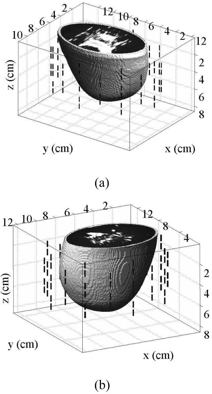
The computational testbeds each consist of an anatomically realistic 3-D numerical breast phantom surrounded by 40-element antenna array comprised of 1.4-cm-long dipoles with a 2 mm source gap. (a) A numerical breast phantom derived from an MRI of a patient with scattered fibroglandular breast tissue, as classified according to the BI-RAD system. (b) A numerical breast phantom derived from the MRI of a patient with heterogeneously dense breast tissue.

A. Numerical Breast Phantoms

The numerical breast phantoms are derived from 3-D MRI datasets from two patients with different breast tissue density classifications, based on the American College of Radiology's [30] BI-RAD system. The first phantom is classified as having “scattered fibroglandular” breast tissue and is illustrated by the 3-D model in Fig. 1(a) and the cross sections of Fig. 2. The second phantom is classified as having “heterogeneously dense” breast tissue and is illustrated by the 3-D model in Fig. 1(b) and the cross sections of Fig. 3. The orthogonal cross sections displayed in Figs. 2 and 3 pass through the center of a 1-cm-diameter spherical inclusion that has been added to each phantom to represent a malignant lesion.

Fig. 2.

Relative permittivity and effective conductivity of the scattered fibroglandular 3-D numerical breast phantom at 1.5 GHz. Cross-sections are shown through the center of the malignant inclusion. (a) ϵ_r in y-z plane, (b) ϵ_r in x-z plane, (c) ϵ_r in x-y plane, (d) σ_eff in y-z plane (S/m), (e) σ_eff in x-z plane (S/m), (f) σ_eff in x-y plane (S/m).

Fig. 3.

Relative permittivity and effective conductivity of the heterogeneously dense 3-D numerical breast phantom at 1.5 GHz. Cross-sections are shown through the center of the malignant inclusion. (a) ϵ_r in y-z plane, (b) ϵ_r in x-z plane, (c) ϵ_r in x-y plane, (d) σ_eff in y-z plane (S/m), (e) σ_eff in x-z plane (S/m), (f) σ_eff in x-y plane (S/m).

The numerical breast phantoms are created following the procedures reported in [23], [44], [45]. The intensity of the voxels in each MRI dataset is converted to dispersive dielectric properties via a piecewise linear mapping. A single-pole Debye model (7) is used to describe the frequency-dependent behavior of the dielectric properties of all of the biological tissues in the computational model. We choose a spatially-invariant relaxation time constant of τ = 17.5 ps for FDTD algorithmic simplicity and efficiency. The frequency dependence of the complex permittivity of the constituent tissues is illustrated in Fig. 4, and their Debye parameters are listed in Table I. The interior of each breast phantom is segmented into three distinct regions: adipose, fibroglandular, and transition. We adopt the dielectric properties reported in a recent large scale dielectric spectroscopy study [11] for the adipose and fibroglandular regions in our models. MRI voxel intensities in these two regions are mapped to +/- 40% ranges about the mean Debye parameters given in Table I. Voxels in the transition region are mapped to the range spanning the maximum of the adipose range to the minimum of the fibroglandular range. The Debye parameters for adipose tissue are derived by first averaging all of the Cole-Cole curves from the large-scale tissue study [11] that correspond to breast tissue samples with 85-100% adipose tissue (denoted “Group 3” in [11]), and then fitting a Debye model with τ = 17.5 ps to the averaged curve over the frequency range of 500 MHz to 3.5 GHz. The Debye parameters for fibroglandular tissue result from applying the same procedure to the “Group 2” Cole-Cole curves from [11].

Fig. 4.

Frequency dependence of the single-pole Debye tissue models used in the numerical breast phantoms. (a) ϵ_r and (b) σ_eff . The curves for adipose and fibroglandular tissues represent the mean of the full mapping range from the raw MRI data.

TABLE I.

Debye parameters of the media modeled in the computational testbeds (valid for the frequency range of 0.5 to 3.5 ghz)

Material	ε ∞	Δ ε	σs (S/m)	τ (ps)
Adipose tissue (mean)	4.68	3.21	0.0881	17.5
Fibroglandular tissue (mean)	17.3	19.4	0.535	17.5
Dry skin	18.4	21.9	0.737	17.5
Malignant inclusion	23.2	33.6	0.801	17.5
Coupling medium	2.6	0.0	0.0	17.5

The 2-mm-thick skin layer is modeled using the dielectric properties for dry skin [38] which we approximate with the Debye parameters given in Table I. The dielectric properties assigned to the spherical inclusions are adapted from a recent study [31] and are representative of malignant breast tissue properties in our frequency range of interest. The cross sections of Figs. 2 and 3 show the dielectric properties at 1.5 GHz for each phantom. The auxiliary differential equation (ADE) approach is used to incorporate Debye dispersion into the FDTD simulations, and the boundary conditions consist of the dispersive media formulation of the Uniaxial Perfectly Matched Layer (UPML) [29]. We also use FDTD as the forward solver within our DBIM algorithm. However, the spatial resolutions of the data generation and forward solver FDTD simulations are not the same. The grid cell dimension for the data-generation FDTD simulations is L = 0.5 mm, while L = 2.0 mm for the forward solver.

We generate patient-specific bases by the method of Section III-A using the specific Gaussian functions defined therein. We choose N_x = N_y = N_z = 10 functions per axis for both phantoms to provide basis resolution on the order of 1 cm. Applying the procedure to the scattered fibroglandular numerical breast phantom reduces 29,108 voxels (L = 2.0 mm) to 665 patient-specific basis functions. For the heterogeneously dense phantom, the procedure reduces 30,787 voxels (L = 2.0 mm) to 691 patient-specific basis functions. The basis functions are arranged by the SVD procedure in order of increasing spatial variation, as illustrated by the two representative patient-specific basis functions of the scattered fibroglandular phantom shown in Fig. 5.

Fig. 5.

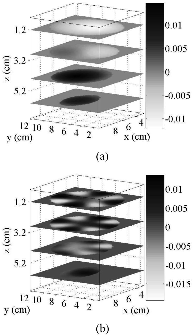
Examples of the patient-specific basis functions used to reduce the dimension of the inverse scattering problem. Each plot shows four x-y cross sections of two of the real-valued basis functions. These examples were generated for the interior of the scattered fibroglandular breast phantom with N_x = N_y = N_z = 10, and correspond to the (a) 2^nd and (b) 29^th of 665 basis functions.

Both the design of the patient-specific basis functions and the FDTD forward solver require an estimate of the location of the breast surface and the thickness of the skin layer.In our testbeds, this information is obtained by taking the known skin region in each numerical breast phantom and downsampling by a factor of four in each dimension to the L = 2.0 mm resolution. In practice, the breast surface could be estimated using the UWB microwave surface-sensing technique reported in [46]. Alternatively, technologies such as laser-video triangulation or time-of-flight laser scanning can be used. Breast skin thickness can be approximated using published studies [47] or radar signal processing techniques [48]. We further assume that the dispersive dielectric properties of the skin layer are known and we incorporate those properties into the FDTD forward solver. This is a reasonable assumption since the contrast between wet and dry skin has been shown to be only about 10% [38].

B. Antenna Array, Data Acquisition, and Calibration

Figure 1 illustrates the configuration of a 40-element cylindrical antenna array that surrounds each breast phantom. The array consists of five elliptical rings of eight electrically-small dipole antennas. The ring diameters are chosen to minimize the size of the computational domains while ensuring that no antenna is closer than 1 cm to the surface of the breast phantom. The ring diameters of the array for the scattered fibroglandular phantom are (9.6×12.4 cm) and for the heterogeneously dense phantom are (10.4 × 11.6 cm). The ring spacing in the z-dimension is 1 cm for both array configurations. Each dipole antenna is modeled by two 6 mm segments of copper wire separated by a 2 mm gap. Coupling between array elements is minimized by rotating the placement of the dipoles in vertically adjacent rings by 22.5°.

An FDTD simulation is conducted for each antenna in the array. In each simulation, one antenna array element is excited with a modulated Gaussian pulse (-20 dB bandwidth: 500 MHz to 3.5 GHz) applied to the feed point of the z-directed dipole antenna. The -20 dB bandwidth of the radiated signal 5 cm away in the coupling medium is 875 MHz to 3.75 GHz. The z-directed electric fields at the feed points of the other antennas in the array are recorded and transformed to phasors at the frequencies of interest via an on-the-fly discrete Fourier transform (DFT) computation [29].

As noted in Section IV-A, the grid cell dimensions for the data-generation and forward FDTD models are different. This results in an inherent mismatch between the two sets of simulations. The data and the forward solution will disagree by as much as 15% even when the same distribution of dielectric properties is simulated. We note that this adds an element of error to our experiments since we are not committing the so-called “inverse crime” [15]. The mismatch is partially corrected through the use of the calibration procedure proposed by Meaney et al. [1]. Both sets of FDTD calibration simulations are run for the case where the antenna array is immersed alone in the coupling medium. The calibration procedure consists of finding a complex-valued correction factor for each transmit-receive pair in the array, such that the two sets of calibration simulations agree. The correction factors are then applied to the output of the forward solver at each iteration of the DBIM. We also note that the two sets of FDTD simulations are run on different platforms. The data-generation FDTD simulations are run in parallel on a computing cluster, while the forward solver is run on a desktop computer utilizing Acceleware hardware acceleration technology [49].

V. RESULTS

We first compare the imaging performance of the single-frequency, voxel-based DBIM to that of our patient-specific basis approach. We then present results for the patient-specific basis approach using multiple-frequency DBIM, for which it is not computationally practical to implement a voxel-based approach. In the examples considered in this section, the patient-specific basis functions are sampled on the original voxel-based mesh, although as noted in Section II-B this does not have to be the case in general. For all the numerical examples of Section V-B, we have added white Gaussian noise to the simulated measurements with a signal to noise ratio (SNR) of 60 dB relative to the total signal. This SNR is considerably higher than the SNR reported in experimental microwave breast imaging systems [1].

A. Comparison of Voxels and Patient-Specific Basis Functions

We have applied a single-frequency DBIM algorithm for both the voxel-based and the patient-specific basis approaches. Data is simulated at 1.5 GHz for the heterogeneously dense numerical breast phantom of Figs. 1(b) and 3. This phantom has 30,787 voxels and 691 patient-specific basis functions. The frequency of 1.5 GHz was chosen to balance imaging resolution against algorithm stability. We have applied a two-stage algorithm similar to the multiple-frequency algorithm described in Section II-D, with the difference being that for the single-frequency case we solve (3) and (6) for the complex unknowns ο and φ instead of solving (8) for the real-valued Debye parameters. The average dielectric properties of the breast interior estimated by the homogeneous stage of the algorithm need only be found once since this step is mathematically equivalent for both the voxel-based mesh and the patient-specific basis. The algorithms were terminated after four iterations for both the homogeneous and heterogeneous estimation stages, which was sufficient to achieve convergence in each case.

The two resulting distributions are nearly identical qualitatively, as illustrated by the cross sections shown in Fig. 6. To quantify this comparison, we observe that a comparable scattering residual is achieved by each method. The voxel-based approach reduced the norm of b(ω) to a value slightly smaller than that reached with the patient-specfic basis function approach, a phenomenon we attribute to the extra degrees of freedom in the voxel-based mesh [22]. We also evaluate the root mean squared (RMS) difference between the voxel and patient-specific basis reconstructions over all voxels in the breast volume. At 1.5 GHz, the RMS difference between the reconstructions of relative permittivity is 1.74 and the RMS difference between the reconstructions of effective conductivity is 0.115 S/m. There is a substantial lack of correlation between the spatial distribution of the permittivity and conductivity estimates of Fig. 6, both of which differ substantially from the true profile of Fig. 3. In particular, the estimated conductivity distribution exhibits greater qualitative error relative to the true spatial profile of Fig. 3 than does the estimated permittivity distribution. The poorer performance of the reconstruction of the conductivity profile in breast imaging has previously been discussed [50] and underscores the importance of implementing a multiple-frequency solution. However, these results show excellent agreement between the voxel-based and patient-specific basis solutions.

Fig. 6.

A comparison of the distributions reconstructed by the single-frequency DBIM using patient-specific basis functions and voxels for the heterogeneously dense breast phantom. The estimated 3-D distribution of relative permittivity and effective conductivity at 1.5 GHz are shown in x-y cross sections at z = 2.4 cm. (a) patient-specific basis estimate of ϵ_r, (b) voxel estimate of ϵ_r, (c) patient-specific basis estimate of σ_eff (S/m), (d) voxel estimate of σ_eff (S/m).

B. Multiple-Frequency DBIM with Patient-Specific Basis Functions

We now apply the multiple-frequency DBIM to the simulated data from each numerical breast phantom at six frequencies (1.2, 1.5, 1.8, 2.1, 2.4, and 2.7 GHz). Each phantom is simulated both with and without a 1-cm-diameter malignant inclusion positioned adjacent to areas of fibroglandular heterogeneity as shown in Figs. 2 and 3. The voxel-based mesh requires over 2.5 GB to store the multiple-frequency matrix M in single-precision for each of the breast phantoms. This amount would increase substantially if additional antenna measurements or frequencies were considered, or if a more complicated dispersion model were used e.g., estimating all four Debye parameters). With the use of the patient-specific basis functions, the storage of M requires only about 60 MB for each phantom. Given the computational limitations of the desktop computer on which we run the DBIM (2.01 GHz AMD Athlon64 processor with 2 GB RAM), we do not attempt to solve the multiple-frequency problem with the voxel-based approach. We only show results when the patient-specific basis functions are used.

The 3-D reconstruction of the complex permittivity profile obtained by applying the multiple-frequency DBIM to the scattered fibroglandular phantom is illustrated in Fig. 7 by the 2-D orthogonal cross sections passing through the center of the inclusion. These images were created by converting the estimated 3-D spatial profile of Debye parameters to relative permittivity and effective conductivity at 1.5 GHz. The estimated properties distribution in the area of the inclusion is limited by the resolution of the system and is influenced by scattering contributions from the surrounding heterogeneous tissue, resulting in a smearing of the reconstructed inclusion. In addition, the orientation and vertical span of the cylindrical array result in a smearing of the reconstructed distribution along the z-axis.

Fig. 7.

Estimated 3-D distributions of relative permittivity and effective conductivity of the scattered fibroglandular phantom at 1.5 GHz. The distribution was estimated using 665 patient-specific basis functions and noisy data at 1.2, 1.5, 1.8, 2.1, 2.4, and 2.7 GHz. 2-D cross-sections are shown through the known center of the malignant inclusion. (a) ϵ_r in y-z plane, (b) ϵ_r in x-z plane, (c) ϵ_r in x-y plane, (d) σ_eff in y-z plane (S/m), (e) σ_eff in x-z plane (S/m), (f) σ_eff in x-y plane (S/m).

The 1-D transections of Fig. 8, taken through the center of the inclusion, further illustate a significantly underestimated reconstruction relative to the true profile of the phantom. The effect of the inclusion on the reconstruction is demonstrated in Fig. 8 by comparison of the sample 1-D transection of the phantom and reconstruction both with and without the inclusion. It is important to note that although such transections serve as a useful spot check and a convenient profile comparison, they are inherently limited in assessing the quality of the full 3-D image. Alternatively, subtraction of the full 3-D reconstructions with and without an inclusion reveals a compact contrast at the site of the inclusion, as shown in the 2-D difference images in the coronal plane in Fig. 9 (a) and (c), where the marker shows the location of the center of the inclusion in the phantom. The peak values of the difference profile at the inclusion site at 1.5 GHz are 9.5 in ϵ_r and 0.29 S/m in σ_eff.

Fig. 8.

A sample 1-D comparison of the true phantom dielectric profile and the reconstructed profile, for the scattered fibroglandular phantom with and without a malignant inclusion. The 1-D cuts through the interior breast volume are taken along the line y = 5.2 cm, z = 2.2 cm, passing through the center of the inclusion. (a) ϵ_r, (b) σ_eff (S/m).

Fig. 9.

Images of the difference between multiple-frequency reconstructions of numerical breast phantoms with and without a malignant inclusion. The difference in relative permittivity and effective conducivity at 1.5 GHz are shown in x-y cross sections at z = 2.4 cm. The known center of the inclusion is marked with a white 'x'. (a) difference in Ƞ_r for the scattered fibroglandular phantom, (b) difference in Ƞ_r for the heterogeneously dense phantom, (c) difference in σ_eff for the scattered fibroglandular phantom (S/m), (d) difference in σ_eff for the heterogeneously dense phantom (S/m).

The heterogeneously dense breast phantom (Fig. 3) presents a more challenging detection problem due to the extensive fibroglandular breast tissue within the phantom. The reconstruction of the complex permittivity profile obtained by applying the multiple-frequency DBIM to this phantom is shown in Fig. 10. In comparison to Fig. 7, the 2-D cross-sections of the 3-D reconstruction for this denser phantom exhibit a larger area of elevated dielectric properties, corresponding to the higher normal fibroglandular tissue content of this phantom. The presence of the malignant inclusion is obscured in the images due to the limited resolution available from the system and the density of the fibroglandular tissue, which exhibits dielectric properties very similar to that of malignant tissues [11], [31]. Despite the obfuscation of the effect of the inclusion, subtraction of the full 3-D reconstructions of the phantom with and without an inclusion again reveals a compact contrast at the site of the inclusion. 2-D cross sections of the difference in the coronal plane are shown in Fig. 9 (b) and (d), where the marker shows the location of the center of the inclusion in the phantom. The peak values of the difference profile at the inclusion site at 1.5 GHz are 8.2 in ϵ_r and 0.27 S/m in σ_eff.

Fig. 10.

Estimated 3-D distributions of relative permittivity and effective conductivity of the heterogeneously dense phantom at 1.5 GHz. The distribution was estimated using 691 patient-specific basis functions and noisy data at 1.2, 1.5, 1.8, 2.1, 2.4, and 2.7 GHz. 2-D cross-sections are shown through the known center of the malignant inclusion. (a) ϵ_r in y-z plane, (b) ϵ_r in x-z plane, (c) ϵ_r in x-y plane, (d) σ_eff in y-z plane (S/m), (e) σ_eff in x-z plane (S/m), (f) σ_eff in x-y plane (S/m).

Our two-stage approach to the multiple-frequency DBIM takes seven iterations to converge for both phantoms: four iterations for the average properties estimation, and three iterations for the estimation of the dielectric profile. Each iteration is completed in 42 minutes on average. This computation time is broken down as follows. The dispersive FDTD simulations running on the Acceleware card in the desktop computer [49] takes approximately 32 seconds per transmitting antenna for a total of 22 minutes. This time includes an on-the-fly discrete Fourier transform calculation for all voxels inV every eight time steps [29]. About 14 minutes are needed for file I/O and the construction of M. The remaining 6 minutes are used to choose the regularization parameter, solve (8), and update the distributions of Debye parameters. In addition, the custom patient-specific basis must be created once per phantom and this process takes on the order of four minutes, depending on the size of the phantom. The computation time of the FDTD forward solution is the largest computational expense, and could be further reduced through parallel use of the FDTD accelerator hardware. We also note that our DBIM code is not optimized. For example, the main body of the DBIM code (written in MATLAB) currently transfers data via text files to and from a C++ code that accesses the accelerator card. Computation time could be further reduced by interfacing the card directly with MATLAB.

VI. CONCLUSION

We have presented a method for enhancing the computational efficiency of 3-D multiple-frequency microwave breast imaging. The multiple-frequency approach improves the conditioning of the inverse problem and enhances the resolution of the reconstruction. In addition, reconstruction of a frequency dependent model offers an inherent correlation between the real and imaginary parts of the complex permittivity. The importance of such behavior is evidenced by the presence of a correlation, both spatially and in magnitude, in actual tissue distributions as well as the lack of spatial correlation often seen in single-frequency reconstructions. Reducing the dimension of the inverse scattering problem relaxes the computational constraints and allows the consideration of a larger number of frequencies and measurements as compared to the solution of the problem on a fine voxel-based mesh. Specifically, we have proposed the use of patient-specific basis functions to reduce the dimension of the inverse scattering problem. The basis functions conform to the interior volume of the breast and are designed to represent details on the order of the resolution limits of the system. The conformal shape and the smoothness of these continuous basis functions avoid the discretization errors encountered by some other methods of dimensional reduction, while offering a reduction in dimension of nearly two orders of magnitude. We have showed using a single-frequency example that the resolution and profile distribution that can be reconstructed with the patient-specific basis is substantially similar to that of a high resolution voxel-based mesh.

We have explored the performance of our 3-D multiple-frequency microwave breast imaging algorithm using two realistic computational testbeds. The testbeds consist of a high resolution numerical breast phantom derived from a 3-D MRI dataset, and represent two BI-RADS classifications of breast tissue distributions. The combined use of the fine detail available from the MRIs and data from the most recent and comprehensive dielectric properties studies results in highly realistic numerical breast phantoms.

Our 3-D microwave imaging results point to the challenge of tumor detection via the reconstruction of dielectric properties distributions in the breast interior. The electrically small features of the true profile are underestimated and the contribution to the reconstruction from even a scattered distribution of fibroglandular heterogeneity interferes with the ability to distinctly image the inclusion. These challenges are magnified for distributions such as the heterogeneously dense breast phantom. Irrespective of the detection challenges, the imaging results demonstrate the utility of this 3-D method to applications such as the characterization and monitoring of tissue distribution and density for all classifications of breast tissue.

In order to evaluate the information available from the presence of a malignant inclusion, we have also compared reconstructions with and without the inclusion. Differential images formed by subtracting two 3-D reconstructions (with and without the inclusion) clearly and accurately locate the inclusion; 1-D transections of the two 3-D reconstructions also illustrate the impact of the inclusion on the estimated dielectric properties. It is premature to assess whether the formation of a differential microwave image for the purpose of cancer detection is clinically feasible. Baseline reconstructions of healthy breasts become less valid with time, as factors such as aging and image registration can cause a change in the distribution of normal breast tissues. Differential imaging is potentially applicable to contrast-enhanced microwave breast cancer detection, whereby contrast agents are introduced alter the dielectric properties of malignant tissue [51], [52]. Such a method would consider two successive scans of the patient's breast before and after the introduction of the agents, such that the differential image will reveal the presence of the contrast agent that has accumulated in the tumor.

REFERENCES

- [1].Meaney PM, Fanning MW, Li D, Poplack SP, Paulsen KD. A clinical prototype for active microwave imaging of the breast. IEEE Trans. Microw. Theory Tech. 2000;48(11):1841–1853. [Google Scholar]
- [2].Bulyshev AE, Semenov SY, Souvorov AE, Svenson RH, Nazarov AG, Sizov YE, Tatsis GP. Computational modeling of three-dimensional microwave tomography of breast cancer. IEEE Trans. Biomed. Eng. 2001 Sep;48(9):1053–1056. doi: 10.1109/10.942596. [DOI] [PubMed] [Google Scholar]
- [3].Zhang ZQ, Liu QH, Xiao CJ, Ward E, Ybarra G, Joines WT. Microwave breast imaging: 3-D forward scattering simulation. IEEE Trans. Biomed. Eng. 2003;50(10):1180–1189. doi: 10.1109/TBME.2003.817634. [DOI] [PubMed] [Google Scholar]
- [4].Kooij BJ. Topical Meeting on Biomedical EMC, 16th International Zurich Symposium on Electromagnetic Compatibility. Zurich; Switzerland: Feb, 2005. Non-linear microwave tumor imaging in a heterogeneous female breast; pp. 53–58. [Google Scholar]
- [5].Meaney PM, Fanning MW, Raynolds T, Fox CJ, Fang QQ, Kogel CA, Poplack SP, Paulsen KD. Initial clinical experience with microwave breast imaging in women with normal mammography. Academic Radiology. 2007 Feb;14(2):207–218. doi: 10.1016/j.acra.2006.10.016. [DOI] [PMC free article] [PubMed] [Google Scholar]
- [6].Meaney PM, Fang Q, Kogel CA, Poplack SP, Kaufman PA, Fox CJ, Paulsen KD. Proc. EuCAP 2006. Nice; France: Nov, 2006. Microwave imaging for neoadjuvant chemotherapy monitoring. [Google Scholar]
- [7].Chaudhary SS, Mishra RK, Swarup A, Thomas JM. Dielectric properties of normal and malignant human breast tissues at radiowave and microwave frequencies. Indian J. Biochem. and Biophys. 1984;21:76–79. [PubMed] [Google Scholar]
- [8].Surowiec AJ, Stuchly SS, Barr JR, Swarup A. Dielectric properties of breast carcinoma and the surrounding tissues. IEEE Trans. Biomed. Eng. 1988;35:257–263. doi: 10.1109/10.1374. [DOI] [PubMed] [Google Scholar]
- [9].Campbell AM, Land DV. Dielectric properties of female human breast tissue measured in vitro at 3.2 GHz. Phys. Med. Biol. 1992;37(1):193–210. doi: 10.1088/0031-9155/37/1/014. [DOI] [PubMed] [Google Scholar]
- [10].Joines WT, Dhenxing YZ, Jirtle RL. The measured electrical properties of normal and malignant human tissues from 50 to 900 MHz. Med. Phys. 1994;21:547–550. doi: 10.1118/1.597312. [DOI] [PubMed] [Google Scholar]
- [11].Lazebnik M, McCartney L, Popovic D, Watkins CB, Lindstrom MJ, Harter J, Sewall S, Magliocco A, Booske JH, Okoniewski M, Hagness SC. A large-scale study of the ultrawideband microwave dielectric properties of normal breast tissue obtained from reduction surgeries. Phys. Med. Biol. 2007;52:2637–2656. doi: 10.1088/0031-9155/52/10/001. [DOI] [PubMed] [Google Scholar]
- [12].Li X, Bond EJ, Van Veen BD, Hagness SC. An overview of ultrawideband microwave imaging via space-time beamforming for early-stage breast cancer detection. IEEE Antennas Propag. Mag. 2005 Feb;47:19–34. [Google Scholar]
- [13].Fear EC. Microwave imaging of the breast. Technology in Cancer Research and Treatment. 2005 Feb;4(1):69–82. doi: 10.1177/153303460500400110. [DOI] [PubMed] [Google Scholar]
- [14].Kerlikowske K. The mammogram that cried Wolfe. N. Engl. J. Med. 2007 Jan;356(3):297–300. doi: 10.1056/NEJMe068244. [DOI] [PubMed] [Google Scholar]
- [15].Colton D, Kress R. Inverse Acoustic and Electromagnetic Scattering Theory. 2nd ed. Springer-Verlag Berlin Heidelberg; New York: 1998. [Google Scholar]
- [16].Cui TJ, Chew WC. Inverse scattering of two-dimensional dielectric objects buried in a lossy earth using the distorted Born iterative method. IEEE Trans. Geosci. Remote Sens. 2001;39(2):339–346. [Google Scholar]
- [17].Rekanos IT, Raisanen A. Microwave imaging in the time domain of buried multiple scatterers by using an FDTD-based optimization technique. IEEE Trans. Magn. 2003;39(3):1381–1384. [Google Scholar]
- [18].Li D, Meaney PM, Paulsen KD. Conformal microwave imaging for breast cancer detection. IEEE Trans. Microw. Theory Tech. 2003;51(4):1179–1186. [Google Scholar]
- [19].Takenaka T, Zhou H, Tanaka T. Inverse scattering for a three-dimensional object in the time domain. Journal of the Optical Society of America: A. 2003;20(10):1867–1874. doi: 10.1364/josaa.20.001867. [DOI] [PubMed] [Google Scholar]
- [20].Zhang ZQ, Liu QH. Three-dimensional nonlinear image reconstruction for microwave biomedical imaging. IEEE Trans. Biomed. Eng. 2004;51(3):544–548. doi: 10.1109/TBME.2003.821052. [DOI] [PubMed] [Google Scholar]
- [21].Bulyshev AE, Souvorov AE, Semenov SY, Posukh VG, Sizov YE. Three-dimensional vector microwave tomography: Theory and computational experiments. Inverse Problems. 2004;20:1239–1259. [Google Scholar]
- [22].Fang Q, Meaney PM, Paulsen KD. Singular value analysis of the Jacobian matrix in microwave image reconstruction. IEEE Trans. Antennas Propag. 2006;54(8):2371–2380. [Google Scholar]
- [23].Winters DW, Bond EJ, Veen BDV, Hagness SC. Estimation of the frequency-dependent average dielectric properties of breast tissue using a time-domain inverse scattering technique. IEEE Trans. Antennas Propag. 2006;54(11 (2)):3517–3528. [Google Scholar]
- [24].Paulsen KD, Meaney PM, Moskowitz MJ, Sullivan JM. A dual mesh scheme for finite-element based reconstruction algorithms. IEEE Trans. Med. Imag. 1995 Sep;14(3):504–514. doi: 10.1109/42.414616. [DOI] [PubMed] [Google Scholar]
- [25].Baussard A, Miller EL, Lesselier D. Adaptive multiscale reconstruction of buried objects. Inverse Problems. 2004;20:S1–S15. [Google Scholar]
- [26].Brandstatter B, Hollaus K, Hutten H, Mayer M, Merwa R, Scharfetter H. Direct estimation of Cole parameters in multifrequency EIT using a regularized Gauss-Newton method. Physiological Measurement. 2003 May;24(2):437–448. doi: 10.1088/0967-3334/24/2/355. [DOI] [PubMed] [Google Scholar]
- [27].Fang Q, Meaney PM, Paulsen KD. Microwave image reconstruction of tissue property dispersion characteristics utilizing multiple-frequency information. IEEE Trans. Microw. Theory Tech. 2004;52(8):1866–1875. [Google Scholar]
- [28].Chew W. Waves and Fields in Inhomogeneous Media. IEEE Press; Piscataway, NJ: 1995. [Google Scholar]
- [29].Taflove A, Hagness SC. Computational Electrodynamics: The Finite-Difference Time-Domain Method. 3rd ed. Artech House; Norwood, MA: 2005. [Google Scholar]
- [30].American College of Radiology [Online]. Available: http://www.acr.org.
- [31].Lazebnik M, Popovic D, McCartney L, Watkins CB, Lindstrom MJ, Harter J, Sewall S, Ogilvie T, Magliocco A, Breslin TM, Temple W, Mew D, Booske JH, Okoniewski M, Hagness SC. A large-scale study of the ultrawideband microwave dielectric properties of normal, benign, and malignant breast tissues obtained from cancer surgeries. Phys. Med. Biol. 2007;52:6093–6115. doi: 10.1088/0031-9155/52/20/002. [DOI] [PubMed] [Google Scholar]
- [32].Chew WC, Wang YM. Reconstruction of 2-dimensional permittivity distribution using the distorted Born iterative method. IEEE Trans. Med. Imag. 1990;9(2):218–225. doi: 10.1109/42.56334. [DOI] [PubMed] [Google Scholar]
- [33].Bulyshev AE, Souvorov AE, Semenov SY, Svenson RH, Nazarov AG, Sizov YE, Tatsis GP. Three-dimensional microwave tomography. Theory and computer experiments in scalar approximation. Inverse Problems. 2000;16:863–875. [Google Scholar]
- [34].Semenov SY, Bulyshev AE, Abubakar A, Posukh VG, Sizov YE, Souvorov AE, van den Berg PM, Williams TC. Microwave-tomographic imaging of the high dielectric-contrast objects using different image-reconstruction approaches. IEEE Trans. Microw. Theory Tech. 2005 Jul;53(7):2284–2294. [Google Scholar]
- [35].Semenov SY, Bulyshev AE, Souvorov AE, Nazarov AG, Sizov YE, Svenson RH, Posukh VG, Pavlovsky AV, Repin PN, Tatsis GP. Three-dimensional microwave tomography: Experimental imaging of phantoms and biological objects. IEEE Trans. Microw. Theory Tech. 2000 Jun;48(6):1071–1074. [Google Scholar]
- [36].Fang Q, Meaney PM, Geimer SD, Streltsov AV, Paulsen KD. Microwave image reconstruction from 3-D fields coupled to 2-D parameter estimation. IEEE Trans. Medical Imag. 2004;23(4):475–484. doi: 10.1109/tmi.2004.824152. [DOI] [PubMed] [Google Scholar]
- [37].Lazebnik M, Okoniewski M, Booske JH, Hagness SC. Highly accurate Debye models for normal tissue dielectric properties at microwave frequencies. IEEE Microw. Wireless Compon. Lett. 2007 Dec;17(12):822–824. [Google Scholar]
- [38].Gabriel S, Lau RW, Gabriel C. The dielectric properties of biological tissues: III. Parametric models for the dielectric spectrum of tissues. Phys. Med. Biol. 1996;41:2271–2293. doi: 10.1088/0031-9155/41/11/003. [DOI] [PubMed] [Google Scholar]
- [39].Remis RF, van den Berg PM. On the equivalence of the newton-kantorovich and distorted born methods. Inv. Prob. 2000;16(1):1–4. [Google Scholar]
- [40].Tikhonov AN, Arsenin VT. Solutions of Ill-Posed Problems. Winston; Washington, D.C.: 1977. [Google Scholar]
- [41].Hansen PC, O'Leary DP. The use of the L-curve in the regularization of discrete ill-posed problems. SIAM J. Sci. Comput. 1993;14(6):1487–1503. [Google Scholar]
- [42].Mallat S. A Wavelet Tour of Signal Processing. 2nd ed. Academic Press; San Diego, CA: 1999. [Google Scholar]
- [43].Golub GH, Loan CFV. Matrix Computations. 3rd ed. John Hopkins University Press; Baltimore, MD: 1996. [Google Scholar]
- [44].Davis SK. Ph.D. dissertation. University of Wisconsin - Madison; Madison, WI: Aug, 2006. Ultrawideband radar-based detection and classification of breast tumors. [Google Scholar]
- [45].Converse M, Bond EJ, Van Veen BD, Hagness SC. A computational study of ultrawideband versus narrowband microwave hyperthermia for breast cancer treatment. IEEE Trans. Microw. Theory Tech. 2006;54(5):2169–2180. [Google Scholar]
- [46].Winters DW, Shea JD, Madsen EL, Frank GR, Van Veen BD, Hagness SC. Estimating the breast surface using UWB microwave monostatic backscatter measurements. IEEE Trans. Biomed. Eng. 2008 Jan;55(1):247–256. doi: 10.1109/TBME.2007.901028. [DOI] [PubMed] [Google Scholar]
- [47].Pope TL, Read ME, Medsker T, Buschi AJ, Brenbridge AN. Breast skin thickness: Normal range and causes of thickening shown on film-screen mammography. Journal of The Canadian Association of Radiologists. 1984;35:365–368. [PubMed] [Google Scholar]
- [48].Williams TC, Fear EC, Westwick DT. Tissue sensing adaptive radar for breast cancer detection - investigations of an improved skin-sensing method. IEEE Transactions on Microwave Theory and Techniques. 2006 [Google Scholar]
- [49].Acceleware Corp. [Online]. Available: http://www.acceleware.com.
- [50].Meaney PM, Yagnamurthy NK, Paulsen KD. Pre-scaling of reconstruction parameter components to reduce imbalance in image recovery process. Phys. Med. Biol. 2002;47:1101–1119. doi: 10.1088/0031-9155/47/7/308. [DOI] [PubMed] [Google Scholar]
- [51].Lazebnik M, Booske JH, Hagness SC. Dielectric-properties contrast enhancement for microwave breast cancer detection: Numerical investigations of microbubble contrast agents. to be presented at the XXIX General Assembly of the International Union of Radio Science (URSI); Chicago, IL. 2008. [Google Scholar]
- [52].Mashal A, Booske JH, Hagness SC. Towards contrast-enhanced microwave-induced thermoacoustic imaging of breast cancer: An experimental study of the effects of microbubbles on simple thermoacoustic targets. Phys. Med. Biol. doi: 10.1088/0031-9155/54/3/011. submitted. [DOI] [PMC free article] [PubMed] [Google Scholar]