How Multiple Conductances Determine Electrophysiological Properties in a Multicompartment Model

Abstract

Most neurons have large numbers of voltage- and time-dependent currents that contribute to their electrical firing patterns. Because these currents are nonlinear, it can be difficult to determine the role each current plays in determining how a neuron fires. The lateral pyloric (LP) neuron of the stomatogastric ganglion of decapod crustaceans has been studied extensively biophysically. We constructed ∼600,000 versions of a four-compartment model of the LP neuron and distributed 11 different currents into the compartments. From these, we selected ∼1300 models that match well the electrophysiological properties of the biological neuron. Interestingly, correlations that were seen in the expression of channel mRNA in biological studies were not found across the ∼1300 admissible LP neuron models, suggesting that the electrical phenotype does not require these correlations. We used cubic fits of the function from maximal conductances to a series of electrophysiological properties to ask which conductances predominantly influence input conductance, resting membrane potential, resting spike rate, phasing of activity in response to rhythmic inhibition, and several other properties. In all cases, multiple conductances contribute to the measured property, and the combinations of currents that strongly influence each property differ. These methods can be used to understand how multiple currents in any candidate neuron interact to determine the cell's electrophysiological behavior.

Introduction

The mixture of voltage- and calcium-dependent channels and their distribution across the surface of a neuron collectively determine the electrophysiological properties of the neuron, including its resting membrane potential, input impedance, firing rate in response to current, and the extent to which it exhibits neuronal behaviors such as bursting, plateauing, and postinhibitory rebound (Marder, 1998). For a neuronal network to function properly, the neurons in that network must exhibit network-appropriate behaviors.

Recent work has shown that although a neuron may behave similarly from animal to animal, the densities of voltage-gated channels can vary severalfold from animal to animal (Golowasch and Marder, 1992a; Golowasch et al., 2002; MacLean et al., 2005; Schulz et al., 2006, 2007). How, then, is reliable neuronal behavior maintained in the face of this variability? One possible answer is that although conductances are variable, they are variable in a correlated manner, and these correlations preserve the function of the neuron. This idea was given additional plausibility by the discovery that many channels are expressed in a correlated manner, at least at the level of mRNA (Schulz et al., 2006, 2007).

We sought to examine the hypothesis that correlations between conductances are required to conserve the electrophysiological function of neurons. We generated a large population of models of a single identified neuron, the lateral pyloric (LP) neuron, found in the stomatogastric ganglion (STG) of the crab Cancer borealis. We generated this population by choosing model parameters at random and filtering out models that did not behave appropriately. We then measured a number of electrophysiological properties in the resulting models and looked for correlations between model parameters that were induced by our constraints on electrophysiological properties.

Historically, a number of different approaches have been used to assess the role of a given channel in a given electrophysiological property of a neuron. One such approach is pharmacological blockade (Hille, 2001). Although this can be done successfully, it presupposes both that a given drug's cellular targets are known and that it is selective. Often, neither of these conditions is met. More recently, many have studied the effects of genetically altering or deleting currents on neuronal dynamics (Raman et al., 1997; Khaliq et al., 2003; MacLean et al., 2003; Swensen and Bean, 2005). Again, although these manipulations are often informative, their interpretation is complicated by compensatory mechanisms that occur during development. A third method is to use the dynamic clamp to add or subtract a current from a neuron (Prinz et al., 2004a).

The most common computational technique used to assess the role of a given parameter on the behavior of a neuron is sensitivity analysis (Butera et al., 1999; Hill et al., 2001, 2002; Jezzini et al., 2004). Here, we used a different approach to understand the extent to which combinations of neuronal conductances influence a number of different neuronal behaviors and compare this approach to sensitivity analysis.

Materials and Methods

Electrophysiology

Experiments were performed essentially as described previously (Goaillard et al., 2004). All preparations had two intact superior esophageal nerves and included the esophageal ganglion, but they had from zero to two intact inferior esophageal nerves.

Modeling voltage-gated currents

The LP neuron models contained 10 voltage- and calcium-gated currents. These were the delayed-rectifier potassium current (I_Kd); the transient potassium current (I_A); the calcium current (I_Ca); the calcium-activated potassium current (I_KCa); the hyperpolarization-activated inward current (I_h); the proctolin-activated current (I_pr), a mixed inward current that is activated by several neuromodulators, including proctolin (Swensen and Marder, 2000); the fast sodium current (I_Na); the axonal delayed-rectifier potassium current (I_Kda); and the axonal transient potassium current (I_Aa). The I_A current was modeled as the sum of a fast and a slow component (I_Af and I_As), but the maximal conductances of these currents were held in a fixed ratio (0.885:1), because they model a single voltage-gated current as characterized physiologically. The model contained two leak currents, I_leak (the somatoneuritic leak) and I_leak,ax (the axonal leak conductance), both described by the usual formalism but with different maximal conductances.

The mathematical description of most of these currents (I_Kd, I_A, I_Ca, I_KCa, I_h, and I_pr) was based on descriptions in previous work (Buchholtz et al., 1992; Golowasch and Marder, 1992b), but with several revisions. In all cases, we tuned the half-activation voltages and kinetics of these currents to provide good fits to voltage-clamp data (Golowasch and Marder, 1992a; Turrigiano et al., 1995; Schulz et al., 2006). The axonal currents (I_Na, I_Kda, and I_Aa) were based on those in the Connor-Stevens model of crab walking leg axon (Connor et al., 1977), but the half-activation and kinetic parameters of these currents were tuned to have the desired current-clamp behavior in the baseline model (see below, Construction of baseline model). Finally, there were three synaptic currents in the final LP neuron models, representing synaptic inputs from other members of the pyloric network: I_synAB, I_synPD, and I_synPY. They are described below.

All model currents except I_Ca were modeled as ohmic currents, described by the following equation:

where ḡ is the maximal conductance, w is the product of the gating variables raised to the appropriate powers, v is the membrane potential, and E is the reversal potential. The reversal potential of each current in the model depended on the permeant ions. The reversal potential was +55 mV for sodium currents, −80 mV for potassium currents (including I_synPD), −25 mV for I_h, −10 mV for I_pr, and −70 mV for I_synAB and I_synPY.

The calcium current was modeled using the Goldman-Hodgkin-Katz equation, and was given by the following:

where

P̄_Ca is the maximal calcium permeability, m_Ca is the calcium channel activation, h_Ca is the calcium channel inactivation, N_A is Avogadro's number (6.022 × 10²³ mol⁻¹), q_e is the elementary charge (1.602 × 10⁻⁷ pC), z_Ca is the valence of a calcium ion (+2), [Ca²⁺]_i is the internal calcium concentration, [Ca²⁺]_o is the external calcium concentration (13 mm), k is Boltzmann's constant (1.381 × 10⁻²³ J/K), and T is the temperature in Kelvin (283.15°K = 10°C).

In the model, we assumed that I_Ca and I_KCa channels were clustered together, and each cluster was associated with a calcium microdomain (Marrion and Tavalin, 1998; Fakler and Adelman, 2008). We know of no evidence either for or against this hypothesis in the STG, but it seems to be common in other systems (Fakler and Adelman, 2008). The maximal permeability of I_Ca was related to the per-cluster maximum permeability by the following:

and the maximal conductance of I_KCa was related to the per-cluster maximal conductance by the following:

where ρ_clust is the density of clusters (in clusters/nF), P̄_Ca¹ is the per-cluster maximal permeability of I_Ca, and ḡ_KCa¹ is the per-cluster maximal conductance of I_KCa. We simulated the accumulation of Ca²⁺ in an (average) small volume associated with each microdomain. The equation governing intracellular calcium was as follows:

where [Ca²⁺]_∞ is the steady-state calcium concentration in the absence of calcium current (20 μm), τ_Ca is the time constant of calcium buffering (70.4 ms), and V_Ca is the volume associated with each microdomain (6.49 μm³).

In generating our population of models, we picked values of P̄_Ca and ḡ_KCa at random and solved Equations 5 and 6 for ρ_clust and ḡ_Ca¹, assuming a fixed P̄_Ca¹ of 1.1675 × 10⁻³ μm³/ms. One consequence of this scheme is that an increase in P̄_Ca alone will not change the dynamics of calcium accumulation (because the calcium accumulation is done on a per-microdomain basis, and increasing P̄_Ca increases the density of microdomains but not the dynamics within a microdomain) and therefore will not change the dynamics of I_KCa. Another approach would be to make ρ_clust, P̄_Ca¹, and ḡ_Ca¹ all be independently tunable parameters, but this seemed overly complex given the experimental uncertainties about the mechanics of calcium accumulation in this system.

Equations for the steady-state (in)activation and time constants of each voltage- and calcium-gated current are given in Table 1.

Table 1.

Equations governing the voltage dependence and kinetics of currents in the LP model

The first column gives the name of the current, the second column gives the form of the gating factor (w; see Materials and Methods, Modeling voltage-gated currents), the third column gives the steady-state activation, the fourth column gives the time constant of activation, the fifth column gives the steady-state inactivation, and the sixth column gives the time constant of inactivation. Membrane potentials (v) are in millivolts, internal calcium concentration ([Ca]_i) is in micromolars, and time constants (τ_m, τ_h) are in milliseconds. The function lgc(x) is equal to 1/[1 + exp(− x)], and linoid(x) is equal to x/[exp(x) − 1]. The parameter v_½,pr was chosen at random when sampling the parameter space. In the baseline model, it had a value of −45 mV.

Modeling synaptic currents

During the pyloric rhythm, the LP neuron receives inhibition from three main sources: the anterior burster (AB) neuron, the pyloric dilator (PD) neurons, and the pyloric (PY) neurons. In the model, we approximated these inputs by fixed rhythmic patterns of synaptic conductance.

The synapses from AB and PY to LP are glutamatergic, predominately chloride-mediated, and rapid (Hartline and Gassie, 1979; Eisen and Marder, 1982; Marder, 1984). The synapse from PD to LP, in contrast, is cholinergic, potassium-mediated, and slow (Eisen and Marder, 1982; Marder and Eisen, 1984). To reflect this, the model AB and PY synapses had instantaneous dynamics and a reversal potential of −70 mV, and the PD synapse had slower dynamics (with a fixed time constant of 50 ms) and a reversal potential of −80 mV (the K⁺ reversal potential in the model). Each synapse was driven by a fixed presynaptic voltage waveform with a typical pyloric period of 1 s. These were based on smoothed recordings of AB (for the AB and PD synapses) and PY (for the PY synapse), which were then subjected to Fourier analysis. The presynaptic voltage used for the AB and PD synapses was as follows:

where v_AB/PD is in millivolts, t is in seconds, and f₀ = 1 Hz, the fundamental frequency of the simulated rhythm. Similarly, the presynaptic voltage used for the PY synapse was as follows:

For all synapses, the synaptic conductance was then given by the following equations:

where g_syn is the synaptic conductance, ḡ_syn is the maximal synaptic conductance, s is the fractional activation of the synapse, τ_syn is the synaptic time constant, v_pre is the presynaptic voltage, v_thresh is the synaptic threshold, and v_scale sets the voltage sensitivity of the synapse. s_∞(x) is the Naka-Rushton function, given by 1/(1 + x⁻²) for x > 0, and 0 otherwise. For the AB and PD synapses, v_thresh = −58 mV and v_scale = 15 mV. For the PY synapse, v_thresh = −53 mV and v_scale = 3 mV. For the AB and PY synapses, τ_syn = 0 ms, and for the PD synapse, τ_syn = 50 ms.

Construction of baseline model

Once we had established reasonable descriptions of the intrinsic and synaptic currents in the LP neuron, we next wanted to establish a morphology for the model that mimicked the morphology of the biological LP and captured some rudimentary aspects of its electrophysiology. Additionally, we feared that a “brute force” search of possible morphologies and possible conductance distributions would be prohibitively time consuming. We therefore built a “baseline” model that was similar to LP in a number of ways: it had a morphology grossly consistent with the biological LP, it had spikes that were generated distally and were greatly attenuated in the soma, its input impedance was similar to that of LP (data not shown), its spike-frequency versus voltage curve was similar to that of LP, and it had voltage-gated currents similar to those of LP.

In developing the baseline model, we started with the simplest possible model and added complexity as needed to agree with the data. We eventually settled on a four-compartment model (Fig. 1) that combined a good fit to the impedance over a range of frequencies (0.1–200 Hz), a reasonable spike height as recorded in the soma (∼9 mV), and a reasonable resting membrane potential (approximately −40 mV).

Figure 1.

Circuit diagram of model. Each rectangle is an electrical compartment. Conductance abbreviations in each rectangle indicate which conductances were present in that compartment. All conductances were present at uniform density across the soma, near neurites, and far neurites compartments.

We then added the reformulated voltage-gated conductances to the soma and neurite compartments of the four-compartment model (Fig. 1). Somatoneuritic currents (I_leak, I_Kd, I_A, I_Ca, I_KCa, I_h, and I_pr) were present at uniform density in the soma and neurite compartments and were absent elsewhere. The synaptic currents were present at uniform density only in the neurite compartments, and the axonal currents (I_leak,ax, I_Na, I_Kda, and I_Aa) were present only in the axon compartment. All of these distributions are simplified versions of the true channel distributions in biological LP neurons (Hartline and Graubard, 1992; Baro and Harris-Warrick, 1998; Baro et al., 2000; French et al., 2004), but they are likely to be reasonable approximations at the level of detail we are interested in at present. The maximal conductances of most voltage-gated conductances were set to values close to those seen in the voltage-clamp recordings. The single exception to this was ḡ_KCa, which was set to a value ∼40% of the value seen in voltage-clamp recordings. We found that increasing ḡ_KCa beyond this value led to endogenous bursting, which is not usually observed in the isolated LP in C. borealis. (It is not entirely clear why this is the case, but we suspect that the published voltage-clamp recordings were traces chosen for their large currents and that single LP neurons may not have all currents simultaneously large.)

Because the resulting model had physiological behavior that approximately matched that of the biological LP, with grossly reasonable maximal conductances, we declared this model an acceptable baseline model for later sampling of the parameter space. We note that the baseline model is not itself an admissible LP model. In particular, it bursts too late in the cycle in response to pyloric-like input, and the spike frequency during the burst is too low. This necessitated the use of sampling to generate admissible LP models (see Results, Production of LP model population).

All simulations of the baseline and sampled models were performed using NEURON (Carnevale and Hines, 2005) as a simulation engine, which was called from Matlab (Mathworks). Unless noted otherwise, the CVODE integration method was used with an absolute tolerance of 25 μV for voltage, 10 nm for internal [Ca²⁺], and 0.001 for gating variables.

“Measuring” electrophysiological properties of models

We measured the electrophysiological properties of models under three different conditions: a small voltage-clamp step, to assess input conductance; no input, to assess spontaneous activity; and a pattern of rhythmic synaptic inhibition, to mimic the input the LP neuron receives during the ongoing pyloric rhythm. These inputs were delivered to each model cell, and the output of the cell was analyzed to measure the various electrophysiological properties. All of the codes for managing the simulations, checking whether their responses had come to steady state, and characterizing the resulting model behaviors were written in the Matlab scripting language.

First condition: small voltage-clamp step.

The cell soma was clamped to −60 mV and allowed to come to steady state. The soma potential was then stepped to −65 mV for 150 ms, a typical step duration used in experimental protocols to measure input conductance. The difference in steady-state current, ΔI, between the holding potential and the test potential was then divided by the potential difference, Δv = −5 mV, to obtain the input conductance, G_in. For this stimulus, the sodium conductance, proctolin-activated conductance, and synaptic conductances were all zeroed, to simulate the conditions in which these measurements were made experimentally. Additionally, an electrode-induced shunt (with a conductance of 15 nS and a reversal potential of −35 mV) was included in the models for this protocol only, because an electrode-induced shunt in the experiments will clearly have a strong effect on measurements of G_in. Because simulation of voltage clamp necessitates the solution of a stiff set of differential equations (Carnevale and Hines, 2005), this protocol was run using the backward Euler integration method, and a time step of 25 μs.

Second condition: no current injection.

This condition simulates the spontaneous activity of a neuron that has been isolated from pyloric inputs but still receives descending modulatory inputs. Therefore, the synaptic conductances were zeroed, but the proctolin-activated conductance and the sodium conductance were not. We simulated this condition until the model came to apparent steady state and computed a number of features based on its steady-state waveform. These include the qualitative type of activity (silent, periodic spiker, aperiodic spiker, periodic nonspiker, or aperiodic nonspiker); the minimum, maximum, mean, and SD of the soma potential, axon potential, and somatic Ca²⁺ concentration; the number of spikes; the spike frequency; the mean spike duration; the mean and SD of the interspike intervals; the duration of the burst; the minimum, maximum, mean, and SD of the slow-wave somatic potential (the somatic potential if spikes are deleted, interpolated over, and the resulting waveform is low-pass filtered); the maximum spike height; and the cycle period. Some of these are only applicable for some qualitative activity types.

Third condition: periodic synaptic inhibition.

Each model was subjected to a pattern of rhythmic synaptic inhibition that approximates what the LP neuron receives during the ongoing pyloric rhythm (see above, Modeling synaptic currents). In this condition, no conductances were zeroed. The synaptic currents were injected into the model until it reached apparent steady state, and the same scalar properties described above were computed based on the steady-state waveform in this condition.

In more detail, the synaptic inputs were provided to each model for several cycles, using the same initial conditions as used for the spontaneous activity. After each cycle, the last cycle was compared with the penultimate cycle to determine whether the model had come to steady state. To be considered at steady state, four quantities had to be approximately equal on the last and the penultimate cycle: mean somatic voltage, SD of somatic voltage, mean somatic [Ca²⁺], and SD of somatic [Ca²⁺]. Voltages (both mean and SD) were considered “approximately equal” if they differed by <0.1 mV, and Ca²⁺ concentrations were considered approximately equal if they differed by <0.01 μm.

Statistics

To test whether two parameters were significantly correlated in the population of 1304 LP models, we calculated the correlation coefficient (r) between the two parameters and used a permutation test to determine whether the calculated r differed significantly from zero. A significance level of α = 0.001 was used for each pair of parameters to facilitate comparison with Schulz et al. (2007).

Cubic fits

To develop a simple description of how a particular electrophysiological property depends on the model parameters, we fit cubic functions to a set of “data” consisting of a population of LP models. Each model had a set of parameters (maximal conductances, etc.) and a number of electrophysiological properties (resting membrane potential, slow-wave amplitude in response to rhythmic inhibition, etc.). One property at a time was fit, and each was treated as a scalar function of the parameters. To put all parameters on a common scale, each parameter was “z-scored” (the mean value of the parameter in the LP model population was subtracted off, and the SD was then divided out) before fits were performed.

A quadratic polynomial in 17 variables has 17 + 2 choose 17 = 171 terms, each with an associated coefficient, and a full cubic model has 17 + 3 choose 17 = 1140 terms/coefficients. A polynomial with a small number of coefficients will generally have good generalization performance but may not be able to fit the target function well. A polynomial with a large number of coefficients will be better able to fit the target but may suffer from overfitting and therefore not generalize well (Hastie et al., 2001). To have finer-grained control over the number of coefficients (and thus the fit-quality/generalization tradeoff), we used a subset of the 1140 possible terms, selected using a cross-validation procedure.

The LP models were first divided into a training set (90%) and a test set (10%). We used fivefold cross-validation on the training set to determine a set of terms that were likely to have an optimal fit on novel models. We varied the number of terms, starting with a single constant term, and added terms until we found a set of terms that gave the lowest cross-validation error. The next term to add was determined by temporarily adding all terms that could be obtained by increasing the degree of an existing term by 1 (not going beyond cubic terms), fitting the resulting polynomial to all of the training data, and retaining the most significant novel term (as determined by a t test). For this type of procedure, the cross-validation error at first decreases as the number of terms increases, but after a critical number of terms are added, the cross-validation error starts to increase. We then selected the simplest polynomial that had error not significantly worse than the minimum error, as assessed by a t test, and used this as our final polynomial. This was then fit to all of the training set to establish a final set of coefficients, and this fit was evaluated on the test set as a final metric of the quality of the fit. Determining the cubic coefficients involves finding the least-squares solution of a set of equations that is linear in the coefficients. In all cases, the final number of coefficients was much less than the number of data points in the training set (largest number of coefficients was 158, number of training data points was 1174) (see Table 4), so the best-fit cubic coefficients were uniquely determined. SEs for the coefficients were calculated using the usual normal-theory formulas for linear regression (Draper and Smith, 1998).

Table 4.

Polynomial fits to model properties

Property	RMSE for constant fita	Number of coefficientsb	Test RMSEc	Test R2d
Input conductance (nS)	8.69	112	2.88	0.89
Resting membrane potential (mV)	2.12	107	0.48	0.94
Resting spike rate (Hz)	3.44	135	0.82	0.95
Phase of burst onset (%)	3.20	158	1.85	0.70
Phase of burst offset (%)	2.64	30	1.95	0.43
Spike rate in burst (spikes/cycle)	3.40	140	0.92	0.93
Slow-wave amplitude (mV)	3.54	151	0.65	0.96
Peak slow-wave potential (mV)	2.51	122	0.54	0.95

^aThe root mean-squared error (RMSE) for the constant that best fits the model property. This is also equal to the square root of the variance of that property, calculated over all 1304 LP models.

^bThe number of polynomial terms used in the best fit, as determined using cross-validation (see Materials and Methods).

^cThe RMSE for the final polynomial fit, as evaluated on the test set.

^dThe, R² for the final polynomial fit, as evaluated on the test set.

Results

The LP neuron has a complex morphology (Fig. 2A), and it plays a critical role in the pyloric rhythm of decapod crustaceans (Harris-Warrick et al., 1992). The pyloric rhythm consists of three distinct phases: (1) the AB and PD neurons fire a burst of spikes (because of their strong electrical coupling, these neurons are collectively referred to as the “pacemaker kernel”); (2) the LP neuron fires a burst of spikes; and (3) the PY neurons fire a burst of spikes (Fig. 2B). The phase at which the LP neuron fires is remarkably consistent from animal to animal, despite substantial variation in the pyloric frequency across animals (Bucher et al., 2005) (J. M. Goaillard, A. L. Taylor, D. J. Schulz, and E. Marder, unpublished observation). In the crab C. borealis, the waveform of the LP neuron reflects the three phases of the pyloric rhythm: during the first phase, when the pacemaker kernel is active (Fig. 2B, left gray bar), it is deeply hyperpolarized; in the second phase, it fires a burst of spikes; and in the third phase, it is inhibited by the PY neurons, but not as much as during the pacemaker activity (Fig. 2B, right gray bar). The bursting of LP is primarily network driven: when it is synaptically isolated from pyloric inputs, LP fires tonically in C. borealis (Fig. 2C) (Golowasch and Marder, 1992a).

Figure 2.

LP neuron morphology and activity. A, Two-photon laser-scanning confocal microscopy image of the LP neuron. B, Intracellular recording of the LP neuron during the ongoing pyloric rhythm. PD nerve (pdn) and pyloric nerve (pyn) recordings are included to show relative timing of the LP burst. Spikes on the pdn are from the two PD neurons, and the larger spikes on the pyn are from the PY neurons. C, Intracellular recording of the LP neuron when pyloric inputs have been blocked by applying 10⁻⁵ m picrotoxin.

Previous work has shown that mRNA levels for a number of voltage-gated channels in LP are correlated (Schulz et al., 2007). Furthermore, for two of three channel types examined, these subunit mRNA levels correlate with the conductance of the channel (Schulz et al., 2006). To gain insight into whether these sorts of correlations might arise from electrophysiological constraints on LP, we constructed a population of multicompartment models of LP, in which maximal conductances were varied and their effects on electrophysiological properties were examined.

Production of LP model population

To generate the LP model population, we first developed a baseline model (see Materials and Methods) and then generated ∼6 × 10⁵ models with randomized parameters in a large neighborhood around this baseline model (Fig. 3). For maximal conductances and maximal permeabilities, the range of possible values for each was from zero to approximately twice the value in the baseline model, so that each would span a realistic range. [Maximal conductances are found to vary threefold to fourfold in this system (Golowasch and Marder, 1992a; Goldman et al., 2001; Golowasch et al., 2002; Schulz et al., 2006, 2007).] Leak reversal potentials were varied over a 10 mV range centered on their baseline values, somewhat arbitrarily. The half-activation potential of the proctolin-activated conductance (v_1/2,pr) was varied over a 20 mV range centered at −45 mV, approximately consistent with the range observed experimentally (Golowasch and Marder, 1992b; Swensen and Marder, 2000) (Goaillard, Taylor, Schulz, and Marder, unpublished observation). The parameters and their ranges are shown in Table 2. Each parameter was chosen from a uniform distribution within the given range, and each parameter was chosen independently of all other parameters. The capacitances and axial resistances of the model were fixed. This approach is similar to that taken in previous work (Foster et al., 1993; Goldman et al., 2001; Prinz et al., 2003, 2004b; Achard and De Schutter, 2006; Tobin et al., 2006; Hobbs and Hooper, 2008; Weaver and Wearne, 2008).

Figure 3.

Activity of six LP models, chosen at random. A, Spontaneous activity in six LP models, chosen at random. This is the model activity in the absence of synaptic inputs. Somatic potential is shown. B, Activity in response to pyloric-like inputs. Models are the same as in A, with corresponding colors. C, Model parameters for each model, scaled to the ranges used for sampling (see Table 2). Note that the models have very different patterns of maximal conductances and other parameters, despite having grossly similar activity. max, Maximum; min, minimum.

Table 2.

Range of parameters used in random sampling of parameter space

	Parameter	Minimum	Maximum	Units
Soma and neurites	Eleak	−23	−13	mV
	ḡleak	0.001	0.002	μS/nF
	ḡKd	0	0.2	μS/nF
	ḡA	0	0.5	μS/nF
	P̄Ca	0	6	μm3/(ms · nF)
	ḡKCa	0	1	μS/nF
	ḡh	0	0.02	μS/nF
	ḡpr	0	0.008	μS/nF
	v½pr	−55	−35	mV
Neurites	ḡsynAB	0	0.06	μS/nF
	ḡstnPD	0	0.06	μS/nF
	ḡsynPY	0	0.02	μS/nF
Axon	Eleak,ax	−7	+3	mV
	ḡleak,ax	0.2	0.45	μS/nF
	ḡNa	0	600	μS/nF
	ḡKd	0	74	μS/nF
	ḡAa	0	100	μS/nF

For each model, each parameter was drawn independently from a uniform distribution with the given bounds. ḡ_x is the maximal conductance of any current x, E_leak values are leak reversal potentials in the indicated compartments, P̄_Ca is the maximal permeability of the (nonohmic) calcium conductance, and v_½pr is the half-activation potential of the proctolin-activated conductance. During sampling, the capacitances and axial resistances were fixed. See Results, Production of LP model population, for an explanation of how these ranges were chosen.

We chose 594,910 parameter sets in this way and performed simulations on each of the resulting models to measure their electrophysiological properties (see Materials and Methods). Each model was assessed in three different conditions. First, the model was subjected to a small voltage-clamp step. Second, the model was given no input, and its spontaneous behavior was observed. Third, a periodic synaptic input was delivered to mimic the pyloric inputs that LP receives during the ongoing pyloric rhythm. In the voltage-clamp condition, the model's input conductance was measured. In the no-input condition, several properties were measured, including the model's spontaneous activity pattern, its resting membrane potential, and its resting spike rate. In the pyloric-input condition, measurements included the phase of burst onset, the phase of burst offset, the spike rate in the burst, the slow-wave amplitude, the peak slow-wave membrane potential, and the coefficient of variation of the interspike interval in the burst. All properties were automatically measured by the simulation code (see Materials and Methods).

We then examined this population of ∼6 × 10⁵ models and selected only those with properties that were in a range that agreed with those of the biological LP neuron, using the bounds shown in Table 3. To be an acceptable LP model, the model had to (1) spike periodically when deprived of input; (2) have an interspike interval coefficient of variation <0.01 when deprived of input, to ensure that it spiked approximately tonically; (3) fire in a reliable pattern from cycle to cycle in response to the pyloric-like input; and (4) have all properties listed in Table 3 within the bounds given. In most cases, the bounds were chosen to contain the central ∼85% of the experimental data points (see Fig. 4, dashed lines). Resting spike rate was higher than those seen in experiments in which the LP neuron is isolated from pyloric network inputs, but similar to the spike rates within an LP burst. Input conductance was restricted to a range generally lower than previously reported experimentally [because the impedance measurements (data not shown) indicated a DC impedance generally larger than those reported previously], but the ratio between highest and lowest allowed values was similar to the ratio between the upper and lower bound of the central 85% of the experimentally measured values (Golowasch and Marder, 1992a).

Table 3.

Bounds on properties used to define the population of admissible LP model neurons

Property	Lower bound	Upper bound
Input conductance (nS)	36	132
Resting membrane potential (mV)	−47.5	−32.5
Resting spike rate (Hz)	13.1	30.6
Phase of burst onset (%)	32.0	44.0
Phase of burst offset (%)	61.7	74.9
Spike rate in burst (spikes/cycle)	16.3	30.2
Slow-wave amplitude (mV)	12.5	27.5
Peak slow-wave potential (mV)	−47.5	−32.5
ISI coefficient of variation in burst	0	0.25

In most cases, the bounds were chosen to contain the central ∼85% of the experimental data points (see Fig. 4, compare dashed lines, histograms). For more details, see Results, Production of LP model population. ISI, Interspike interval.

Figure 4.

Comparison of pyloric activity in experiment and model. A, Histograms of onset phase of firing in experiment (exp) and models. B–E, Histograms of other properties of LP activity in the pyloric rhythm (exp) and in response to a pyloric-like pattern of synaptic inputs (model). Dashed lines in all panels show the constraints imposed on the model population to yield the LP models (as in Table 3). The y-axis in all panels is the percentage of data points.

Filtering the population of ∼6 × 10⁵ models using these criteria yielded 1304 acceptable models of LP. Traces of model LP activity look reasonable, as shown in Figure 3. Both the spontaneous activity of these models (compare Figs. 2C, 3A) and their activity in response to pyloric-like input (compare Figs. 2B, 3B) look similar to recordings of biological LP neurons. In response to pyloric-like inputs, the model LPs generally displayed a burst phase, a phase in which they were mildly hyperpolarized (during which LP receives PY inhibition), and a phase of deep hyperpolarization (during which LP receives pacemaker inhibition). These same three phases are present in recordings from biological LP neurons (Fig. 2B). Although strongly constrained electrophysiologically, the parameters of these models displayed wide variability (Fig. 3C) (also see below).

Histograms of the constrained properties are generally similar between model and experiment (Fig. 4). Consistent with this, the resting membrane potential (data not shown) was similar to that of the biological LPs (experiment: −46.8 ± 6.5 mV, n = 5; model: −44.1 ± 2.1 mV, n = 1304; mean ± SD). Two additional properties that we did not explicitly constrain at this stage were also consistent with the biology. The height of spikes as measured in the soma was similar between model and experiment (experiment: 7.7 ± 1.8 mV, n = 5; model: 8.0 ± 0.6 mV, n = 1304; mean ± SD). Also, the model impedances all matched the qualitative shape of the experimental impedance from 0.1 to 200 Hz (data not shown).

Weak correlations between pairs of parameters in the population of LP models

We examined whether the constraints imposed on the electrophysiological behavior of model LP neurons was reflected in the distributions of model parameters. Histograms of the model parameters for the 1304 models showed wide variability in most parameters (Fig. 5A). For most parameters, models could be found that spanned the sampled range. That is, when the range was binned into 10 bins, at least one model was found in all bins. Other parameters had restricted ranges in the LP population. The most strongly restricted parameter was ḡ_Aa, which was restricted to about half the sampled range. ḡ_Kda and ḡ_synPY also had restricted ranges.

Figure 5.

Distributions of parameters and pairs of parameters in a population of 1304 model LP cells. A, Histograms of individual parameter values. Each x-axis spans the sampled range. Each y-axis is different. B, Scatterplots of pairs of parameter values. Each scatterplot contains 1304 points, corresponding to each of the LP models. Because each pair of parameters can be plotted either as x versus y or y versus x, the scatterplot matrix is symmetric about the diagonal. Scatterplots with blue/red background displayed a statistically significant positive/negative correlation between the two parameters. Histograms highlighted in yellow are those that arguably correspond to channels that Schulz et al. (2007) found to be positively correlated at the level of mRNA.

Does the population of 1304 model LP neurons exhibit any correlations between pairs of model parameters? This was of particular interest because previous experimental results demonstrated correlations between different voltage-gated conductances, some biophysically and some at the level of channel mRNA values (MacLean et al., 2005; Schulz et al., 2006, 2007). Therefore, we calculated correlation coefficients for each pair of parameters and tested these for significance (Fig. 5B) (see Materials and Methods). We found that correlations between different parameters in the LP population were generally weak (Fig. 5B) (red and blue backgrounds show significant correlations at α = 0.001 for individual comparisons). Although a rather stringent significance level of α = 0.001 was used for individual comparisons [and to facilitate comparison to Schulz et al. (2007)], this corresponds to a family-wise significance level of α = 0.13 (n = 136 comparisons, assuming comparisons are independent), which is rather generous. Of the 136 pairs, 126 (93%) had estimated correlation coefficients between −0.2 and +0.2. The strongest correlation was between ḡ_Na and ḡ_Kda, which had a correlation coefficient (r) of 0.49 ± 0.04 [95% confidence interval (CI)].

To determine whether the observed correlations would likely be detected using typical experimental techniques, we picked a random subset of 20 models and tested for significant correlations (this time using a t test, rather than the more computationally expensive permutation test). n = 20 was chosen because it is a reasonable value of n for these types of experiments. This was repeated 2000 times, each time using a different random subset. A significant correlation (at α = 0.001) between ḡ_Na and ḡ_Kda was found in 12.5 ± 1.5% (95% CI) of trials, and all other pairs were lower than this. Of the 136 pairs examined, 131 (96%) had a chance of discovery of <1%. Together, these results imply that the constraints imposed on the electrophysiological properties of the model LP neurons were not sufficient to induce the strong pairwise correlations observed experimentally. This implies that, at least in the model, strong correlations like those measured experimentally are not required for a population to have the electrophysiological properties of an LP neuron.

The LP models are part of a single “island” in parameter space

We were curious to know whether all of the LP models were part of a single connected island of LP cells in parameter space. That is, is it possible to continuously vary the parameters of one LP model and thereby transform it into any other LP model, and to do so in such a way that all intermediate models are also LP models? We cannot prove mathematically that this is the case, but we have strong circumstantial evidence that all of the LP models are part of a single connected volume in parameter space.

To establish this, we drew a line segment between pairs of models in parameter space and tested four equally spaced points on this line to see whether they also satisfied the criteria for an LP model. If they did, we considered the two models to be connected. In addition, if two models are each connected to a third model, then we considered the original two models to be connected. By performing this test on many pairs of models, we were able to establish that all 1304 LP models are connected to one another, at least provisionally. (Note, however, that it does not imply that the set is convex, and, in fact, we found many pairs of models that had non-LP models on the line between them but that were connected via a path involving one or more intercalated models.) This provides strong evidence that our population of LP cells are all part of a single connected volume of LP cells in parameter space, rather than being in a number of islands of LP models separated by one or more “oceans” of non-LP models.

Polynomial fits of the property functions

It is highly desirable to have a quantitative description of how each parameter in a neuronal model influences each electrophysiological property. The computational model provides such a description only implicitly. A more direct description would be provided by a single equation that computes the magnitude of the electrophysiological property given the parameters. To provide such a description, we performed a multiple regression on each electrophysiological property, using the model parameters as predictors. This approach is similar to approaches used previously (Rabitz and Alis, 1999; Feng et al., 2004, 2006; Feng and Rabitz, 2004; Feng, 2005), but those approaches are not well suited to our LP population because our LP model population was not generated via independent variation of parameters (because of the filtering step). We first tried linear fits and quadratic fits to each electrophysiological property, but neither provided acceptable fits. A linear fit has the property that a given change in parameters will have the same effect on output, independent of the starting parameters; for instance, increasing ḡ_A by 3 μS/nF and ḡ_pr by 1 μS/nF will always increase the slow-wave amplitude by 2 mV, regardless of the starting parameters. This will obviously not be true for many parameter-to-property maps arising in complicated biological systems, and allowing quadratic and higher-order terms in the polynomial fit allows a fit to avoid this constraint.

We then tried cubic fits to each electrophysiological property and found that these performed well: we obtained R² values >0.85 for six of the eight properties we examined (Table 4). This indicates that these six properties, as functions of the parameters, were well approximated by cubic polynomials.

As an example, the coefficients of the fit to one of these, the slow-wave amplitude, are shown in Figure 6. The quality of the fit is shown graphically in Figure 6A, which plots the true slow-wave amplitude in each model versus the slow-wave amplitude “predicted” by the fit. The points are near the identity line, indicating a good fit. Insight into which parameters influence the slow-wave amplitude, and in what way, can be gained by examining the coefficients of the fit. The coefficients of the linear terms in the cubic fit show large contributions from ḡ_A, ḡ_synPD, ḡ_pr, P̄_Ca, ḡ_Aa, ḡ_synAB, and ḡ_leak,ax (Fig. 6B). The sign of these coefficients reveals whether the contribution of that term tends to increase the slow-wave amplitude as that parameter is increased (positive sign), or decrease it (negative sign). Some of these effects are expected: because the PD synapse onto LP acts to hyperpolarize LP during the trough of its oscillation, one would expect that increasing ḡ_synPD would increase the slow-wave amplitude. In addition, because the somatoneuritic I_A current would act to limit the rebound from inhibition, one might expect increasing somatoneuritic ḡ_A to decrease the slow-wave amplitude. Other coefficients were more surprising: the linear coefficient of ḡ_Aa (the axonal form of I_A, which has generally faster kinetics than the somatoneuritic I_A) was large and positive, indicating that increasing ḡ_Aa tends to increase the slow-wave amplitude. This was unexpected and is especially surprising in light of the fact that increasing the somatoneuritic I_A has the opposite effect. We found that this effect was caused primarily by a hyperpolarization of the trough potential in the axon (the lowest point of the slow wave), itself caused by the release from inactivation of I_Aa after the LP burst, which was then passively propagated to the soma. This constitutes a prediction of our model.

Figure 6.

Coefficients of the polynomial fit to slow-wave amplitude. A, Quality of the fit. The slow-wave amplitude of each LP model is plotted versus the polynomial fit for that model. Purple points were used in fitting, and orange points were used for testing (see Materials and Methods). R² for each class of points is given. A perfect fit would have all points along the identity line, shown in black. B, Linear coefficients of the polynomial fit. Coefficients have units of millivolts because parameters were z-scored before fitting (see Materials and Methods). Error bars indicate SE. C, Quadratic coefficients of the fit. D, Cubic coefficients of the fit. Panels with a shaded background correspond to axonal parameters. Parameters with uniformly small coefficients are omitted.

The quadratic coefficients of the cubic fit reveal nonlinear effects of changing model parameters (Fig. 6C). Two different kinds of quadratic terms in the cubic fit are possible: one kind involves the square of a single parameter (along the diagonal in Fig. 6C), and the other involves the product of two different parameters (off the diagonal in Fig. 6C). In the case of the slow-wave amplitude fit, the largest quadratic coefficient was for the square of v_1/2,pr, the half-activation of the proctolin-activated current. The coefficient for this term was negative, meaning that either increasing or decreasing v_1/2,pr, relative to its mean value will tend to decrease the slow-wave amplitude, counteracting somewhat the linear effect of decreasing v_1/2,pr.

Cubic terms in the polynomial also describe nonlinear effects of changing model parameters, but involving products of three parameters, rather than two. These three parameters can all be the same, resulting in terms containing single parameters to the third power, or combinations of different parameters. In the slow-wave amplitude fit, the largest-magnitude cubic coefficient is for the cube of ḡ_synPD, reflecting a nonlinear influence of ḡ_synPD on slow-wave amplitude that somewhat counteracts the linear ḡ_synPD term (because the cubic coefficient is negative whereas the linear coefficient is positive and has a larger magnitude). These sorts of insights into what parameters affect other properties can also be obtained by examining the coefficients of those fits, at least in cases where the fit is good.

Using polynomial fits to quantify the effect of each parameter on each electrophysiological property

We wanted to quantify the overall contribution of each model parameter to determining each of the neuron's electrophysiological properties. We did this by starting with the coefficients of the final fit to a property, and setting all of the model parameters to their mean values. We then set them back to their actual values one parameter at a time and noted how much of the variance in the property was explained with the addition of each parameter, as a fraction of the total variance explained by the complete fit. Typically, the amount of variance accounted for by each parameter varies depending on the order in which parameters are added. Therefore, we repeated this process 3000 times, with a random order each time, and averaged the variance added over all repeats. This yielded a measure of the influence exerted by each parameter on the final fit such that the influence of all parameters summed to 1. These “influence factors” are shown in Figure 7 for each property we examined. Interestingly, we found that essentially all properties are affected by many parameters and that the relative importance of parameters varied from property to property.

Figure 7.

Quantification of the effect of each model parameter on each model property. The area of each circle represents the average amount of variance explained by that parameter, as a fraction of the variance explained by the complete fit, and where the average is taken over many different random orders in which the parameters are added to the fit (see Materials and Methods). The areas of the circles in each row sum to 1. Properties not in bold (phase of burst start/end) should be interpreted with caution, because the cubic fits were of poor quality (see Table 4).

Comparing polynomial fitting to traditional sensitivity analysis

Fitting a polynomial to a model property can be viewed as an alternative to more traditional sensitivity analysis. In sensitivity analysis, one typically starts with a single best model, and then each model parameter is varied, one at a time, and the change in the model property is plotted versus each parameter (Butera et al., 1999; Hill et al., 2001, 2002; Jezzini et al., 2004). In theory, fitting a polynomial gives the same information but also tells one how the model responds to combinations of parameter changes. Nevertheless, we were curious to see how the polynomial fits compared with sensitivity analysis. For individual models in the test set, we varied each parameter ±25% of its original value and performed simulations to see how model properties changed. Voltage parameters were varied ±5 mV. We compared the values in these simulations to the values predicted by the polynomial fit. An example is shown in Figure 8A, for the polynomial fit to the spike rate in the LP burst. This example displays good agreement between the cubic fit and the sensitivity analysis results.

Figure 8.

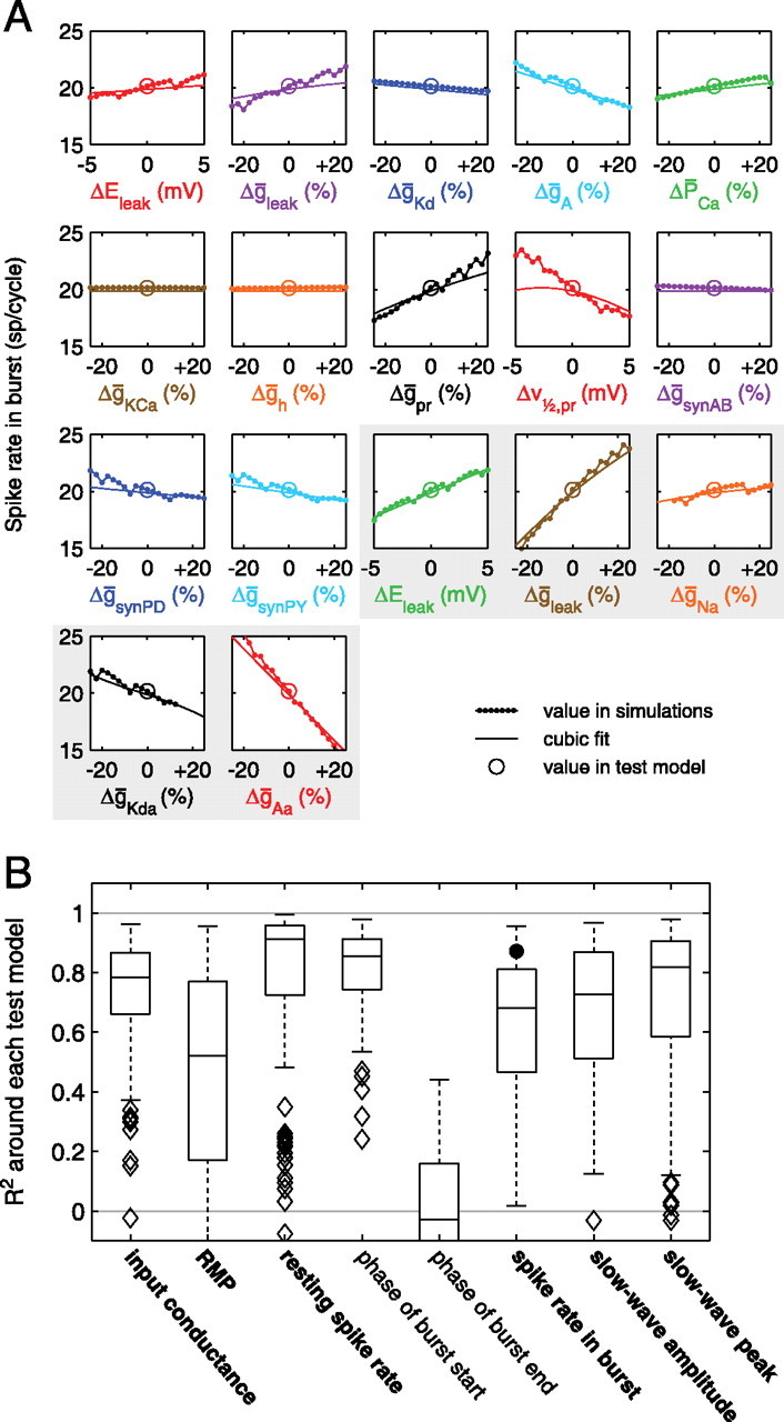
Sensitivity analysis and cubic fits in the neighborhood of test models. A, Each panel shows the result of varying one parameter at a time. Note the close agreement between simulations and the cubic fit in most cases. Missing points in the ḡ_Na and ḡ_Kda panels indicate parameter values for which the models no longer spiked. The gray backdrop indicates axonal parameters. B, Summary of comparisons between sensitivity analysis and cubic fits. Box-and-whisker plots show the distribution of R² values found when comparing the sensitivity data and cubic fits for each property. (The R² values were calculated using only the changes relative to the respective central values; see Results.) Each box-and-whisker plot summarizes the distribution of R² values for all 130 test models. The upper and lower limits of each box give the 75th and 25th percentiles of each distribution, and the line in the middle of each box gives the median. The dashed “whiskers” give the extent of all nonoutlier data points. A data point was classified as an outlier if it was more that 1.5 box heights away from the box. Outliers are shown as diamond symbols. Some properties had a few points with R² values below the lower limit of the plot. The number of such points for the different properties was 5, 17, 0, 0, 58, 8, 2, and 7, respectively. The large black circle indicates the R² value for the example shown in A. Properties not in bold had poor overall R² values (see Table 4).

In many cases, the polynomial fit lines matched the sensitivity analysis curves fairly well (Fig. 8B). To quantify the quality of these fits, we calculated R² values for the cubic fit to each property in the neighborhood of each test model, using data from the sensitivity analysis around each test model. For this analysis, we were mainly interested in how well the cubic fits predicted changes from the property value at the test model, so we subtracted the fit property value at the central model from the fit values and similarly subtracted the simulation property value at the central model from the simulation values. (Failure to perform this step yielded R² values that were generally much lower.) This analysis yielded a range of R² values, but the median across test models was >0.5 for all but one property (phase of burst end, the property for which the cubic fit performed worst overall). This indicates that the cubic fits were able to predict the results of sensitivity analysis fairly well in most cases. However, in some cases, the cubic fits did not predict the sensitivity curves well, as indicated by low or even negative R² values (a negative R² value indicates a fit worse than would be achieved by simply fitting the data by a constant). Although the cubic fits are not a substitute for traditional sensitivity analysis, on the whole the ability of the cubic fits to predict the results of sensitivity analysis were striking, especially because the test models were not used in constructing the fits.

Discussion

How does the combination of voltage-gated conductances in a neuron determine its electrophysiological properties? In this study, we analyzed a population of 1304 model neurons, all of which meet stringent criteria that match those of a specific biological neuron. We found (1) that a population of neurons can have a well constrained electrophysiological phenotype but still display disparate underlying maximal conductances with only weak correlations between conductances and (2) that each property of an identified neuron with well defined behavior is affected by a different set of maximal conductances. These results have implications for the interpretation of experimental results about the effect of neuronal parameters on electrophysiological properties.

Are correlations between maximal conductances required for a given electrophysiological phenotype?

The population of LP models did not show strong correlations between pairs of model parameters, including maximal conductance parameters. This is interesting, because experimental work found strong correlations between mRNA copy numbers for voltage-gated channels in LP and other STG cells (Schulz et al., 2006, 2007). Although in some cases the mRNA levels correlate strongly with conductance magnitudes measured in voltage clamp (Schulz et al., 2006), it is not known whether mRNA copy numbers are well correlated with maximal conductances for all kinds of channels in all neuron classes.

There are two possible explanations for the lack of strong correlations in the model population: either the model fails to capture something important about the neuron's behavior or the neuron's electrical firing properties do not require the correlations seen in the molecular studies. Consistent with the latter explanation, it is possible that the correlations observed experimentally do not arise from electrophysiological constraints, since it is possible to construct LP neurons with conductance ratios other than those observed experimentally and still “act” like LP neurons electrophysiologically. If this were the case, the ratios observed experimentally might be a consequence of the transcriptional regulation of channel genes (Latchman, 1997; Fan et al., 2000; Brivanlou and Darnell, 2002; Rosati and McKinnon, 2004). For instance, having subunits of multiple channel types under the control of a common transcription factor might be simpler than independent transcriptional control of each channel type. This could result in different subunits being expressed in fixed ratios. Thus, the presence of correlations between conductances does not automatically imply that these correlations are required for proper electrophysiological behavior.

Using polynomial fits to capture the relative roles of multiple conductances on neuronal activity

The cubic fits allowed the quantification of the influence of each parameter on each electrophysiological property (Fig. 7). Each property was affected, at least to some extent, by many parameters in the model, but different properties were affected by various parameters to different extents. Recent work on a model of globus pallidus neurons yielded a similar result (Gunay et al., 2008), suggesting that this is a feature common to many neurons.

The large influence of the axonal conductances, and particularly the axonal leak and I_A conductance (ḡ_Aa), on the input conductance was somewhat unexpected. This suggests that, at least in the model, the axon is not as electrically irrelevant to the current–voltage relationship at the soma as might be supposed given the extreme attenuation of spikes in the soma. Although the contributions of multiple parameters on different intrinsic properties were generally different, those for the resting spike rate and the spike rate in the burst were similar. This reflects the fact that these two properties were strongly correlated in the LP model population (data not shown).

Small influence factors should be interpreted with caution; the synaptic conductances (ḡ_synAB, ḡ_synPD, and ḡ_synPY) had small, but nonzero, influence factors for the input conductance, resting membrane potential, and resting spike rate, despite the fact that all of these conductances were set to zero when these properties are measured in the model. This is possible because of high-order correlations between these parameters and parameters that do affect these properties. These correlations are exploited by the fitting routine to give significantly better fits than if the synaptic conductance parameters are not used (data not shown). These potentially misleading influence factors are uniformly small and do not detract from the utility of the influence factors overall.

The finding that each electrophysiological property is determined by a combination of several different conductances (Fig. 7) has important implications for how one interprets experiments involving pharmacological blockers, genetic deletions, and neuromodulation. When the levels of conductances vary from animal to animal, and when an electrophysiological property depends on multiple conductances, blocking one of these conductances may have highly variable effects on that property, because in some animals the conductance may already be low and be compensated for by the other conductances to keep the property at a normal level. A similar argument holds for genetic deletions, but with the added complication that if the deletions are nonacute, the animal may compensate for the knock-out by regulating levels of other conductances (Guo et al., 2000; Zhang et al., 2002; Xu et al., 2003; Zhou et al., 2003). Similarly, neuromodulator effects may vary from preparation to preparation because neuromodulators act on a particular set of conductances, which may be high or low depending on the individual animal.

Approaches to understanding the effect of parameters on electrophysiological properties

In a model, the simplest approach to understanding the effect of parameters on electrophysiological properties is traditional sensitivity analysis: identifying one “best” set of parameters, varying one parameter at a time, and plotting the electrophysiological property of interest against the varied parameter. This approach has been fruitfully applied (Butera et al., 1999; Hill et al., 2001, 2002; Jezzini et al., 2004) but has two limitations: it is based on examining departures from a single model, and it is based on varying one parameter at a time, and therefore yields no information about simultaneously changing multiple parameters.

Another approach is to generate a population of models, either by picking random values for parameters or by systematically scanning the parameter space (Foster et al., 1993; Goldman et al., 2001; Prinz et al., 2003, 2004b; Achard and De Schutter, 2006; Tobin et al., 2006; Hobbs and Hooper, 2008; Weaver and Wearne, 2008). One can then use visualization techniques to determine how electrophysiological properties change as parameters are varied (Ward et al., 1994; Keim, 2000; Taylor et al., 2006), although these techniques are often qualitative and choosing a good method of visualization can be difficult.

In some cases, one can derive closed-form expressions for model properties as functions of parameters (Abbott, 1990), and this is arguably the best solution, when it is possible.

In this work, we used cubic functions to fit electrophysiological properties as a function of model parameters. This allowed a relatively simple description of model behavior over a population of models (not just in the vicinity of a single model), and it described how these models respond to multiple simultaneous parameter changes. Similar methods have been used in the chemistry literature (Rabitz and Alis, 1999; Feng et al., 2004, 2006; Feng and Rabitz, 2004; Feng, 2005) but have not been commonly used to understand neuronal dynamics. We focused here on electrophysiological properties that were real functions of the parameters. For example, the slow-wave amplitude is described by a single real number for each possible choice of parameters. Other cases of interest include properties that are integer (e.g., number of spikes per burst), category (e.g., activity type), or boolean (e.g., spiking or not) functions of the parameters. Fitting polynomials might be useful for integer properties if followed by a rounding operation but would not be ideal for category properties. For these sort of problems, an approach analogous to the one used here would be to use statistical classification (as opposed to regression) techniques (Hastie et al., 2001).

A related problem is finding the set of points in parameter space that all result in the same value for an electrophysiological property (the level set). Olypher and Calabrese (2007) used a numerical approximation to find the level sets of several electrophysiological properties. The method used here offers a more general answer to how parameters affect electrophysiological properties as long as the polynomial fits are sufficiently accurate. The cubic fits used here effectively describe all of the level sets of a particular electrophysiological property.

Relation to previous models of STG neurons

These LP models capture many important features of the biological LP neuron in C. borealis, including the response of LP to pyloric inputs, the attenuation of spikes in the soma, and LP's input impedance. Previous models of LP have captured some of these features but not all of them (Buchholtz et al., 1992; Nowotny et al., 2008). One difference between the behavior of the model and that of the biological LP neuron (Golowasch and Marder, 1992a) is that the model fires more rapidly than the biological neuron at rest, but without this we were not able to obtain the appropriate firing rates in response to inhibitory inputs.

Previous multicompartment models of STG neurons have had only two compartments, one to model the generation of spikes and another that contains the currents typically measured in voltage-clamp experiments (Soto-Trevino et al., 2005; Nowotny et al., 2008). Additional compartments were needed to accurately model both the input impedance of LP (data not shown) and the attenuation of spikes when measured in the soma.

Conclusions

In this work, we found that a population of neurons can have a well constrained electrophysiological phenotype but still display disparate underlying maximal conductances with only weak correlations between conductances, and that each property of an identified neuron with well defined behavior is affected by a different subset of several maximal conductances. These results have important implications for how one interprets experiments involving pharmacological blockers, genetic deletions, and neuromodulation.

References

- Abbott LF. A network of oscillators. J Physics [A] 1990;23:3835–3859. [Google Scholar]
- Achard P, De Schutter E. Complex parameter landscape for a complex neuron model. PLoS Comput Biol. 2006;2:e94. doi: 10.1371/journal.pcbi.0020094. [DOI] [PMC free article] [PubMed] [Google Scholar]
- Baro DJ, Harris-Warrick RM. Differential expression and targeting of K+ channel genes in the lobster pyloric central pattern generator. Ann N Y Acad Sci. 1998;860:281–295. doi: 10.1111/j.1749-6632.1998.tb09056.x. [DOI] [PubMed] [Google Scholar]
- Baro DJ, Ayali A, French L, Scholz NL, Labenia J, Lanning CC, Graubard K, Harris-Warrick RM. Molecular underpinnings of motor pattern generation: differential targeting of shal and shaker in the pyloric motor system. J Neurosci. 2000;20:6619–6630. doi: 10.1523/JNEUROSCI.20-17-06619.2000. [DOI] [PMC free article] [PubMed] [Google Scholar]
- Brivanlou AH, Darnell JE., Jr Signal transduction and the control of gene expression. Science. 2002;295:813–818. doi: 10.1126/science.1066355. [DOI] [PubMed] [Google Scholar]
- Bucher D, Prinz AA, Marder E. Animal-to-animal variability in motor pattern production in adults and during growth. J Neurosci. 2005;25:1611–1619. doi: 10.1523/JNEUROSCI.3679-04.2005. [DOI] [PMC free article] [PubMed] [Google Scholar]
- Buchholtz F, Golowasch J, Epstein IR, Marder E. Mathematical model of an identified stomatogastric ganglion neuron. J Neurophysiol. 1992;67:332–340. doi: 10.1152/jn.1992.67.2.332. [DOI] [PubMed] [Google Scholar]
- Butera RJ, Jr, Rinzel J, Smith JC. Models of respiratory rhythm generation in the pre-Bötzinger complex. II. Populations of coupled pacemaker neurons. J Neurophysiol. 1999;82:398–415. doi: 10.1152/jn.1999.82.1.398. [DOI] [PubMed] [Google Scholar]
- Carnevale NT, Hines ML. The NEURON book. Cambridge, UK: Cambridge UP; 2005. [Google Scholar]
- Connor JA, Walter D, McKown R. Neural repetitive firing: modifications of the Hodgkin-Huxley axon suggested by experimental results from crustacean axons. Biophys J. 1977;18:81–102. doi: 10.1016/S0006-3495(77)85598-7. [DOI] [PMC free article] [PubMed] [Google Scholar]
- Draper NR, Smith H. Applied regression analysis. Ed 3. New York: Wiley; 1998. [Google Scholar]
- Eisen JS, Marder E. Mechanisms underlying pattern generation in lobster stomatogastric ganglion as determined by selective inactivation of identified neurons. III. Synaptic connections of electrically coupled pyloric neurons. J Neurophysiol. 1982;48:1392–1415. doi: 10.1152/jn.1982.48.6.1392. [DOI] [PubMed] [Google Scholar]
- Fakler B, Adelman JP. Control of K(Ca) channels by calcium nano/microdomains. Neuron. 2008;59:873–881. doi: 10.1016/j.neuron.2008.09.001. [DOI] [PubMed] [Google Scholar]
- Fan IQ, Chen B, Marsh JD. Transcriptional regulation of L-type calcium channel expression in cardiac myocytes. J Mol Cell Cardiol. 2000;32:1841–1849. doi: 10.1006/jmcc.2000.1217. [DOI] [PubMed] [Google Scholar]
- Feng XJ. Princeton University; 2005. Optimal identification, analysis, and control of complex bionetworks. PhD thesis. [Google Scholar]
- Feng XJ, Rabitz H. Optimal identification of biochemical reaction networks. Biophys J. 2004;86:1270–1281. doi: 10.1016/S0006-3495(04)74201-0. [DOI] [PMC free article] [PubMed] [Google Scholar]
- Feng XJ, Hooshangi S, Chen D, Li G, Weiss R, Rabitz H. Optimizing genetic circuits by global sensitivity analysis. Biophys J. 2004;87:2195–2202. doi: 10.1529/biophysj.104.044131. [DOI] [PMC free article] [PubMed] [Google Scholar]
- Feng XJ, Rabitz H, Turinici G, Le Bris C. A closed-loop identification protocol for nonlinear dynamical systems. J Phys Chem A. 2006;110:7755–7762. doi: 10.1021/jp056189o. [DOI] [PubMed] [Google Scholar]
- Foster WR, Ungar LH, Schwaber JS. Significance of conductances in Hodgkin-Huxley models. J Neurophysiol. 1993;70:2502–2518. doi: 10.1152/jn.1993.70.6.2502. [DOI] [PubMed] [Google Scholar]
- French LB, Lanning CC, Matly M, Harris-Warrick RM. Cellular localization of shab and shaw potassium channels in the lobster stomatogastric ganglion. Neuroscience. 2004;123:919–930. doi: 10.1016/j.neuroscience.2003.08.036. [DOI] [PubMed] [Google Scholar]
- Goaillard JM, Schulz DJ, Kilman VL, Marder E. Octopamine modulates the axons of modulatory projection neurons. J Neurosci. 2004;24:7063–7073. doi: 10.1523/JNEUROSCI.2078-04.2004. [DOI] [PMC free article] [PubMed] [Google Scholar]
- Goldman MS, Golowasch J, Marder E, Abbott LF. Global structure, robustness, and modulation of neuronal models. J Neurosci. 2001;21:5229–5238. doi: 10.1523/JNEUROSCI.21-14-05229.2001. [DOI] [PMC free article] [PubMed] [Google Scholar]
- Golowasch J, Marder E. Ionic currents of the lateral pyloric neuron of the stomatogastric ganglion of the crab. J Neurophysiol. 1992a;67:318–331. doi: 10.1152/jn.1992.67.2.318. [DOI] [PubMed] [Google Scholar]
- Golowasch J, Marder E. Proctolin activates an inward current whose voltage dependence is modified by extracellular Ca2+ J Neurosci. 1992b;12:810–817. doi: 10.1523/JNEUROSCI.12-03-00810.1992. [DOI] [PMC free article] [PubMed] [Google Scholar]
- Golowasch J, Goldman MS, Abbott LF, Marder E. Failure of averaging in the construction of a conductance-based neuron model. J Neurophysiol. 2002;87:1129–1131. doi: 10.1152/jn.00412.2001. [DOI] [PubMed] [Google Scholar]
- Gunay C, Edgerton JR, Jaeger D. Channel density distributions explain spiking variability in the globus pallidus: a combined physiology and computer simulation database approach. J Neurosci. 2008;28:7476–7491. doi: 10.1523/JNEUROSCI.4198-07.2008. [DOI] [PMC free article] [PubMed] [Google Scholar]
- Guo W, Li H, London B, Nerbonne JM. Functional consequences of elimination of ito,f and ito,s: early afterdepolarizations, atrioventricular block, and ventricular arrhythmias in mice lacking Kv1.4 and expressing a dominant-negative Kv4 alpha subunit. Circ Res. 2000;87:73–79. doi: 10.1161/01.res.87.1.73. [DOI] [PubMed] [Google Scholar]
- Harris-Warrick RM, Marder E, Selverston AI, Moulins M. Dynamic biological networks: the stomatogastric nervous system. Cambridge, MA: MIT; 1992. [Google Scholar]
- Hartline DK, Gassie DV., Jr Pattern generation in the lobster (Panulirus) stomatogastric ganglion. I. Pyloric neuron kinetics and synaptic interactions. Biol Cybern. 1979;33:209–222. doi: 10.1007/BF00337410. [DOI] [PubMed] [Google Scholar]
- Hartline DK, Graubard K. Cellular and synaptic properties in the crustacean stomatogastric nervous system. In: Harris-Warrick RM, Marder E, Selverston AI, Moulins M, editors. Dynamic biological networks: the stomatogastric nervous system. Cambridge, MA: MIT; 1992. pp. 31–86. [Google Scholar]
- Hastie T, Tibshirani R, Friedman J. The elements of statistical learning. New York: Springer; 2001. [Google Scholar]
- Hill AA, Lu J, Masino MA, Olsen OH, Calabrese RL. A model of a segmental oscillator in the leech heartbeat neuronal network. J Comput Neurosci. 2001;10:281–302. doi: 10.1023/a:1011216131638. [DOI] [PubMed] [Google Scholar]
- Hill AA, Masino MA, Calabrese RL. Model of intersegmental coordination in the leech heartbeat neuronal network. J Neurophysiol. 2002;87:1586–1602. doi: 10.1152/jn.00337.2001. [DOI] [PubMed] [Google Scholar]
- Hille B. Ion channels of excitable membranes. Ed 3. Sunderland, MA: Sinauer; 2001. [Google Scholar]
- Hobbs KH, Hooper SL. Using complicated, wide dynamic range driving to develop models of single neurons in single recording sessions. J Neurophysiol. 2008;99:1871–1883. doi: 10.1152/jn.00032.2008. [DOI] [PubMed] [Google Scholar]
- Jezzini SH, Hill AA, Kuzyk P, Calabrese RL. Detailed model of intersegmental coordination in the timing network of the leech heartbeat central pattern generator. J Neurophysiol. 2004;91:958–977. doi: 10.1152/jn.00656.2003. [DOI] [PubMed] [Google Scholar]
- Keim D. An introduction to information visualization techniques for exploring large databases (tutorial). Paper presented at the IEEE Visualization Conference; October; Salt Lake City, UT. 2000. [Google Scholar]
- Khaliq ZM, Gouwens NW, Raman IM. The contribution of resurgent sodium current to high-frequency firing in Purkinje neurons: an experimental and modeling study. J Neurosci. 2003;23:4899–4912. doi: 10.1523/JNEUROSCI.23-12-04899.2003. [DOI] [PMC free article] [PubMed] [Google Scholar]
- Latchman DS. Transcription factors: an overview. Int J Biochem Cell Biol. 1997;29:1305–1312. doi: 10.1016/s1357-2725(97)00085-x. [DOI] [PubMed] [Google Scholar]
- MacLean JN, Zhang Y, Johnson BR, Harris-Warrick RM. Activity-independent homeostasis in rhythmically active neurons. Neuron. 2003;37:109–120. doi: 10.1016/s0896-6273(02)01104-2. [DOI] [PubMed] [Google Scholar]
- MacLean JN, Zhang Y, Goeritz ML, Casey R, Oliva R, Guckenheimer J, Harris-Warrick RM. Activity-independent coregulation of IA and Ih in rhythmically active neurons. J Neurophysiol. 2005;94:3601–3617. doi: 10.1152/jn.00281.2005. [DOI] [PubMed] [Google Scholar]
- Marder E. Roles for electrical coupling in neural circuits as revealed by selective neuronal deletions. J Exp Biol. 1984;112:147–167. doi: 10.1242/jeb.112.1.147. [DOI] [PubMed] [Google Scholar]
- Marder E. From biophysics to models of network function. Annu Rev Neurosci. 1998;21:25–45. doi: 10.1146/annurev.neuro.21.1.25. [DOI] [PubMed] [Google Scholar]
- Marder E, Eisen JS. Transmitter identification of pyloric neurons: electrically coupled neurons use different neurotransmitters. J Neurophysiol. 1984;51:1345–1361. doi: 10.1152/jn.1984.51.6.1345. [DOI] [PubMed] [Google Scholar]
- Marrion NV, Tavalin SJ. Selective activation of Ca2+-activated K+ channels by co-localized Ca2+ channels in hippocampal neurons. Nature. 1998;395:900–905. doi: 10.1038/27674. [DOI] [PubMed] [Google Scholar]
- Nowotny T, Levi R, Selverston AI. Probing the dynamics of identified neurons with a data-driven modeling approach. PLoS ONE. 2008;3:e2627. doi: 10.1371/journal.pone.0002627. [DOI] [PMC free article] [PubMed] [Google Scholar]
- Olypher AV, Calabrese RL. Using constraints on neuronal activity to reveal compensatory changes in neuronal parameters. J Neurophysiol. 2007;98:3749–3758. doi: 10.1152/jn.00842.2007. [DOI] [PubMed] [Google Scholar]
- Prinz AA, Billimoria CP, Marder E. Alternative to hand-tuning conductance-based models: construction and analysis of databases of model neurons. J Neurophysiol. 2003;90:3998–4015. doi: 10.1152/jn.00641.2003. [DOI] [PubMed] [Google Scholar]
- Prinz AA, Abbott LF, Marder E. The dynamic clamp comes of age. Trends Neurosci. 2004a;27:218–224. doi: 10.1016/j.tins.2004.02.004. [DOI] [PubMed] [Google Scholar]
- Prinz AA, Bucher D, Marder E. Similar network activity from disparate circuit parameters. Nat Neurosci. 2004b;7:1345–1352. doi: 10.1038/nn1352. [DOI] [PubMed] [Google Scholar]
- Rabitz H, Alis O. General foundations of high-dimensional model representations. J Math Chem. 1999:197–233. [Google Scholar]
- Raman IM, Sprunger LK, Meisler MH, Bean BP. Altered subthreshold sodium currents and disrupted firing patterns in Purkinje neurons of Scn8a mutant mice. Neuron. 1997;19:881–891. doi: 10.1016/s0896-6273(00)80969-1. [DOI] [PubMed] [Google Scholar]
- Rosati B, McKinnon D. Regulation of ion channel expression. Circ Res. 2004;94:874–883. doi: 10.1161/01.RES.0000124921.81025.1F. [DOI] [PubMed] [Google Scholar]
- Schulz DJ, Goaillard JM, Marder E. Variable channel expression in identified single and electrically coupled neurons in different animals. Nat Neurosci. 2006;9:356–362. doi: 10.1038/nn1639. [DOI] [PubMed] [Google Scholar]
- Schulz DJ, Goaillard JM, Marder EE. Quantitative expression profiling of identified neurons reveals cell-specific constraints on highly variable levels of gene expression. Proc Natl Acad Sci U S A. 2007;104:13187–13191. doi: 10.1073/pnas.0705827104. [DOI] [PMC free article] [PubMed] [Google Scholar]
- Soto-Trevino C, Rabbah P, Marder E, Nadim F. Computational model of electrically coupled, intrinsically distinct pacemaker neurons. J Neurophysiol. 2005;94:590–604. doi: 10.1152/jn.00013.2005. [DOI] [PMC free article] [PubMed] [Google Scholar]
- Swensen AM, Bean BP. Robustness of burst firing in dissociated Purkinje neurons with acute or long-term reductions in sodium conductance. J Neurosci. 2005;25:3509–3520. doi: 10.1523/JNEUROSCI.3929-04.2005. [DOI] [PMC free article] [PubMed] [Google Scholar]
- Swensen AM, Marder E. Multiple peptides converge to activate the same voltage-dependent current in a central pattern-generating circuit. J Neurosci. 2000;20:6752–6759. doi: 10.1523/JNEUROSCI.20-18-06752.2000. [DOI] [PMC free article] [PubMed] [Google Scholar]
- Taylor AL, Hickey TJ, Prinz AA, Marder E. Structure and visualization of high-dimensional conductance spaces. J Neurophysiol. 2006;96:891–905. doi: 10.1152/jn.00367.2006. [DOI] [PubMed] [Google Scholar]
- Tobin AE, Van Hooser SD, Calabrese RL. Creation and reduction of a morphologically detailed model of a leech heart interneuron. J Neurophysiol. 2006;96:2107–2120. doi: 10.1152/jn.00026.2006. [DOI] [PMC free article] [PubMed] [Google Scholar]
- Turrigiano GG, LeMasson G, Marder E. Selective regulation of current densities underlies spontaneous changes in the activity of cultured neurons. J Neurosci. 1995;15:3640–3652. doi: 10.1523/JNEUROSCI.15-05-03640.1995. [DOI] [PMC free article] [PubMed] [Google Scholar]
- Ward MO, LeBlanc J, Tipnis R. N-Land: a graphical tool for exploring n-dimensional data. Paper presented at the CG International Conference; June; Melbourne, Australia. 1994. [Google Scholar]
- Weaver CM, Wearne SL. Neuronal firing sensitivity to morphologic and active membrane parameters. PLoS Comput Biol. 2008;4:e11. doi: 10.1371/journal.pcbi.0040011. [DOI] [PMC free article] [PubMed] [Google Scholar]
- Xu M, Welling A, Paparisto S, Hofmann F, Klugbauer N. Enhanced expression of L-type Cav1.3 calcium channels in murine embryonic hearts from Cav1.2-deficient mice. J Biol Chem. 2003;278:40837–40841. doi: 10.1074/jbc.M307598200. [DOI] [PubMed] [Google Scholar]
- Zhang Z, Xu Y, Song H, Rodriguez J, Tuteja D, Namkung Y, Shin HS, Chiamvimonvat N. Functional roles of Cav 1.3 (alpha1D) calcium channel in sinoatrial nodes: insight gained using gene-targeted null mutant mice. Circ Res. 2002;90:981–987. doi: 10.1161/01.res.0000018003.14304.e2. [DOI] [PubMed] [Google Scholar]
- Zhou J, Kodirov S, Murata M, Buckett PD, Nerbonne JM, Koren G. Regional upregulation of Kv2.1-encoded current, IK,slow2, in Kv1DN mice is abolished by crossbreeding with Kv2DN mice. Am J Physiol Heart Circ Physiol. 2003;284:H491–H500. doi: 10.1152/ajpheart.00576.2002. [DOI] [PubMed] [Google Scholar]