

Abstract
This paper presents several experimental techniques and concepts in the process of measuring mechanical properties of very soft tissue in an ex vivo tensile test. Gravitational body force on very soft tissue causes pre-compression and results in a non-uniform initial deformation. The global Digital Image Correlation technique is used to measure the full field deformation behavior of liver tissue in uniaxial tension testing. A maximum stretching band is observed in the incremental strain field when a region of tissue passes from compression and enters a state of tension. A new method for estimating the zero strain state is proposed: the zero strain position is close to, but ahead of the position of the maximum stretching band, or in other words, the tangent of a nominal stress-stretch curve reaches minimum at λ ≳ 1. The approach, to identify zero strain by using maximum incremental strain, can be implemented in other types of image-based soft tissue analysis. The experimental results of ten samples from seven porcine livers are presented and material parameters for the Ogden model fit are obtained. The finite element simulation based on the fitted model confirms the effect of gravity on the deformation of very soft tissue and validates our approach.
Keywords: Soft tissue modeling, Digital Image Correlation (DIC), Liver tissue, Strain measurement, Mechanical properties, Tension experiment, Zero strain or zero stress reference
1. Introduction
Understanding the mechanical behavior of very soft tissue, such as liver, kidney, brain and prostate, is necessary for developing realistic mathematical models that can be used for computer simulations in surgical planning and training systems. In recent years many attempts have been made to measure the material properties of very soft tissues ex vivo (Miller and Chinzei, 1997; Farshad et al., 1999; Miller, 2001; Chui et al., 2004, 2007; Roan and Vemaganti, 2007), however, the reported experimental data on direct measurement of strain are limited. Typically in such measurements, the force-displacement response of soft tissues was collected. The strain data in soft-tissue was either estimated from the displacement of the machine head (Farshad et al., 1999; Miller, 2001; Chui et al., 2004; Miller, 2005), or determined from the two horizontal markers positioned on the tissue (Chui et al., 2007).
Soft biological tissues are not stress-free in their natural state. They are subjected to gravitational force and also constraints in many cases under physiological conditions. Because the stiffness of very soft tissue is very low around its zero strain state, the deformation due to gravity can be significant. For example, stress due to the weight from 1 cm height of tissue, roughly 100 Pa, can lead to more than 5% of compressive strain to the tissue underneath, according to the stress-strain curves reported for ex vivo porcine brain (Miller and Chinzei, 2002; Miller, 1998) and liver (Chui et al., 2004; Roan and Vemaganti, 2007) tissues. It is well known that stress-strain states on the tissue around the platen or clamps are complicated (Butler et al., 1984; Waldman and Lee, 2005) in an ex vivo test. The effect of gravity field makes the deformation field non-uniform even on the central portion of the tissue. In order to accurately measure the mechanical properties of very soft tissue, some non-contact technique that can measure local strain in the region of interest is needed.
Accurate zero-strain establishment is critical for a nonlinear material test. The effect of a shifted zero strain estimate is not significant at a low strain where the stress-strain curve is relatively linear. However, once the material stiffens at higher strains, a biased zero-strain reference makes a significant difference in the estimated material properties. There are limited reports in the literature about setting the zero strain (or zero stress) state for soft tissues. Combined compression and tension experiments were used in measuring mechanical properties of porcine liver tissue (Chui et al., 2004) and bovine periodontal ligament (Sanctuary et al., 2005). The zero strain point was defined as the middle point in the zero-tangent-zone of the force-strain curve (Sanctuary et al., 2005). Neutral buoyancy measurement was proposed to offset the effect of gravity on human breast (Rajagopal et al., 2007, 2008). The MR images of the breasts immersed in water were acquired and used as the unloaded reference configuration. This method has a problem. Gravity is a body force which acts throughout the volume of the breast, while buoyancy is a surface force exerted only on the interface of water and the breast. Although the net upward buoyancy force could balance the overall weight of the breast, the tissue inside the breast was not stress free. In this paper we propose a purely image-based strain measurement technique to identify the zero strain state for very soft tissue under gravity-induced compression and tensile loading. Instead of the absolute strain field, which was non-uniform and usually unknown in an experiment, the relative or incremental strain field was calculated from images of the deforming tissues. The maximum stretching band on the incremental strain field roughly indicated the zero strain position.
Digital Image Correlation (DIC) is a full-field deformation and strain measurement technique widely used in experimental mechanics (Chu et al., 1985; Sutton et al., 1988; Bruck et al., 1989; Vendroux and Knauss, 1998). Artificially applied speckle patterns or natural texture on a specimen surface are recorded in a experiment. The region being measured on a reference image is mathematically translated, rotated and deformed until the best fit to the region on the deformed image is obtained. The following features of DIC make it suitable for use in the strain measurement of soft tissues: 1) there is no contact with the specimen; 2) natural texture on the bio-tissues can be used for correlation; 3) local strain is measured accurately in the region of interest; 4) this is a direct measurement that does not require recourse to an analytical model; 5) large strain can be measured by correlating of a series of images recorded during the mechanical testing. Previous applications of DIC to biological materials have been reported for measuring the strain of relatively rigid tissues such as cartilage (Wang et al., 2002, 2003) and hoof horn (Zhang and Arola, 2004), or moderately stiff tissues such as arteries (Zhang et al., 2002; Sutton et al., 2008) and joint capsule (Little and Khalsa, 2005). The speckle patterns used for soft tissues were usually generated by spraying quick-drying paint, toner powders, or silicone carbide particles onto the specimen surface. In this paper, the natural texture shown on the surface of porcine liver tissue was used for correlation. A similar marker-less technique has been reported to measure the strain field of heart tissue, namely porcine aortic valves in tension and bovine pericardium tissue in simple shear (Doehring, 2004; Doehring et al., 2004). Texture correlation and strain measurement techniques were also reported for 3D X-ray tomography of trabecular bone (Bay et al., 1999; Liu and Morgan, 2007) and for MR images of tendon (Bey et al., 2002) and intervertebral disc (Gilchrist et al., 2004).
The rest of the paper is organized as follows. In section 2 we present the materials and methods to perform the tissue tension testing, and the formulation as well as the procedure of the global DIC technique. In section 3, we present the results of the experiments, the new method to identify the zero strain state, the material parameters fitted from the experimental data, and the finite element validation. We make concluding remarks and discussions in section 4.
2. Materials and methods
2.1. Specimen preparation
Seven fresh porcine livers were collected from a slaughterhouse and kept frozen in the laboratory. All tissue specimens were cut using a long-bladed knife from frozen porcine liver and remained frozen until the time of the test. The samples were extracted perpendicular to the top surface of the liver and tested in that direction. The outer layer of the liver membrane (capsule) was removed. Samples with large blood vessels or obvious pores were discarded in the experiments, so that the properties of the tissue in the regions that are largely homogeneous were measured.
2.2. Uniaxial tension test
The testing system consists of a uniaxial loading frame with a computer-controlled DC motor and an in-line 2.5 lbf load cell. The top plate, as shown in Figure 1, was mounted on the moving stage; the bottom plate was rigidly fixed to the support of the testing system. The frozen sample, in the shape of rectangular prism with height ~ 25 mm, width and thickness ~ 15 – 17 mm, was attached to the bottom plate by using cyanoacrylate (Super Glue). The glue was then applied on the top of the specimen. The top plate of the testing apparatus was moved down slowly so that it touched the upper surface of the specimen. To assure proper attachment, the tissue close to the two plates was compressed by approximately 1 – 2 mm on each side. The local tissue began to thaw after contacting with the glue and the plates. The specimen was left for about 15 – 30 minutes to thaw at room temperature (~ 22 °C). Water mist was sprayed 2 or 3 times during that time. Upon completion of the thawing process, the tensile test was performed by moving the top platen upwards at 1.27 mm/s, corresponding to a nominal strain rate of about 0.05 s−1. The tests were continued until the glue failed. Images of the deforming liver tissue samples were acquired for later analysis.
Figure 1.
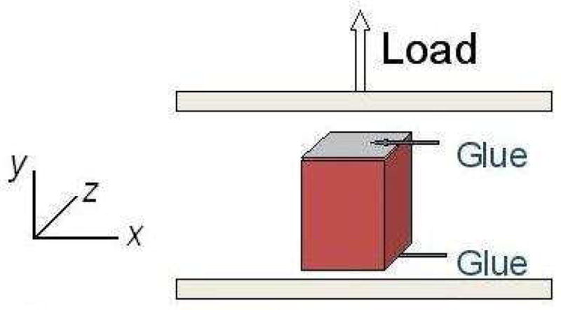
Schematic of the uniaxial tension experiment (Gao et al., 2009).
2.3. Image formation
Digital image correlation requires a random pattern on the sample surface that can be readily identified in sequential images. For very soft tissue, this pattern may be created by spraying paint or powder. Because the tissue samples need to remain wet, it is difficult for paint speckles to adhere onto the tissue, and large deformation and internal strain may cause paint speckles or powders to separate from the tissue in the loading process. The chemical components of the paint may also affect the tissue properties.
Hepatic lobule is the structural unit of a liver. The boundaries of the lobules are defined by connective tissue septa. In a pig, these connective tissue boundaries are very prominent; they are much less clearly defined in humans (Ham, 1969). Figure 2 shows the image of a thawed liver tissue sample before the tensile test. After spraying of water mist, the blood near the surface was diluted and the network of the white connective tissue became visible (see Figure 2). During the process of stretching, the surface roughness was slightly increased and the surface pattern became more distinct, which was desirable for image correlation.
Figure 2.

The image of a liver tissue sample before the uniaxial tension test (Gao et al., 2009).
A Nikon D40X digital camera with a Nikon 18mm-to-55mm f/3.5-to-f/5.6 lens was used to capture the sequential images of the specimen undergoing deformation. The 3872 × 2592 pixels colored images were acquired at 3 frame/s. A B+W polarizer was attached in front of the Nikon lens to reduce the reflection from the wet surface. Two adjustable desk lamps with fluorescent bulbs were used for illumination.
2.4. Global Digital Image Correlation technique
A global version of DIC, i.e. Lagrangian mesh tracing, was utilized in this work. This technique had been developed and used to explore the mechanical properties of open cell aluminum foam in compression (Zhou et al., 2004) and human osteosarcoma cell in shear assay experiments (Cao et al., 2006). The deformation field of the region to be measured was expressed and tracked by the deformation of a mesh which tiled the complete region of interest. Correlations were carried out on sequential image pairs.
2.4.1. Formulation of global DIC
Using the assembling technique of the finite element method, the coordinate xn+1 of a material point in image n+1, can be related to the coordinate of the same point in image n by the following mapping,
| (1) |
where Un is the nodal displacement, the subscript j indicates the nodes in the element where xn is located and is the shape function defined as,
| (2) |
where (xn, yn) are the components of coordinates for the point xn. (Xi, Yi) are coordinates for the corner node Xi of a triangular element. In this paper, X represents the position of a node and U represents the displacement of a node.
The speckle or texture pattern in image n can be expressed as intensity function Fn(xn), which is reconstructed from the gray-scale value of pixels by piecewise bicubic spline interpolation (Bruck et al., 1989). A least-squares type of cost function is then used to define the change in the intensity function value (Wang and Cuitino, 2002) and is given by
| (3) |
where M is the total number of pixels inside the whole meshed region in image n. The first derivative of the cost function, namely the Jacobian matrix, J, can be computed as:
| (4) |
where the derivative is further evaluated using the chain rule
| (5) |
The simplified form of Hessian matrix (Vendroux and Knauss, 1998) H is given by:
| (6) |
Minimization of the cost function can be solved through the use of Newton-Raphson iterations,
| (7) |
where the deformation mapping, Un, is a vector of displacements for all the nodes. H and J are the assembled global matrix and vector, respectively. The solved displacement vector, Un, is used to update the position of the nodes on the (n + 1)th image, which can be used for the correlation of the next image pairs, namely:
| (8) |
where K is the number of the nodes in the mesh.
The accumulated displacement un(x1) for the point xn+1, corresponding to the same material point x1 in image 1, can be expressed as:
| (9) |
These computed displacements are continuous throughout the measured region, since all the nodes on the mesh are connected by element boundaries. The in-plane incremental deformation gradient Fn(xn), for image pair n is:
| (10) |
2.4.2. Calculation of the strain field
In order to create a continuous strain field, the incremental displacement derivative ▽un(xn) is calculated from the interpolation of the averaged nodal displacement derivative (Feng and Rowlands, 1987; Sutton et al., 1991),
| (11) |
where is the average of the nodal displacement derivative, ▽Un, which is calculated from the elements sharing that node:
| (12) |
Assume in image n0, the measured region is at a zero-strain state, then the cumulative Lagrangian strain of point xn, En(xn0), with respect to the zero-strain state in image n0, can be obtained from following equations:
| (13) |
| (14) |
| (15) |
Cn(xn0) is the cumulative right Cauchy-Green tensor,
| (16) |
where is the unit vector in a principle direction in image n0, and λA is the principal stretch ratio with respect to image n0.
2.4.3. Mesh tracing procedures
A fundamental step in all nonlinear minimizations is selection of an accurate starting point. It is essential to select a starting point in the vicinity of a global minimum and avoid local minima. To solve this problem, two sets of coarse-mesh correlations plus one or more sets of fine-mesh correlations, as shown in Figure 3, were run. A coarse mesh has only two 6-node triangular elements. The first coarse mesh covers a region that touches the two plates. The measured positions of two plates were the input to calculate the starting field for the correlation of each image pair. Those plates’ positions were also needed to correlate the images to the corresponding force data. The result from the first set of coarse-mesh correlations was used as the starting field for the correlations of the second coarse-mesh set, which tiles the region of interest. The coarse-mesh correlation is important because a larger correlation window or element has more pixels carrying speckle information, which makes the inside pattern more distinct and hence easier for the correlation to converge. The solved displacement field was used as the starting field for the fine-mesh correlation. In Figure 3, the elements of the fine mesh in image 1 have a nominal side length of 100 pixels. Due to the large deformations of the mesh, some triangular elements could become “skinny”, which may cause poor approximation quality in finite element solutions. To preserve mesh quality, three remeshing steps were taken within the same mesh boundary. Therefore the mesh in image 41 in Figure 3 has more elements than that in image 1.
Figure 3.

Image 1 and image 41 with superimposed three sets of meshes: two coarse and one fine meshes. The coordinates are in pixels.
2.4.4. Method evaluation– translation test
The quality of speckle patterns or textures used for correlation is critical for the measurement. A translation test of a liver tissue sample was carried out to explore the accuracy and resolution of the method. The sample was 15×63×8 mm in height, width and thickness, respectively. The same testing system was used. The tissue sample was glued on an additional plate, which was mounted vertically on top of the moving plate of the loading system. Images were taken when the top plate was moving up at 1.27 mm/s. The correlation was run over a region of 1780×460 pixels. The nominal side length of the fine-mesh elements was 100 pixels, which was used for all the tests. The result was evaluated on a total of 1720 grid points with 20 pixel spacing in either direction over a region of 1720 by 400 pixels (the outermost region was excluded to eliminate the error due to boundary effect (Sutton et al., 1991)). The standard deviation (std) of the displacement for the correlation of a single pair of images was ranged from 0.04 to 0.44 pixels for 15 image-pairs; the average std of the displacement was 0.19 pixel. The average strain was less than 2 × 10⁻³, and the standard deviation of local strains was less than 6 × 10⁻³. Considering the final results of consecutive correlations of 15 image-pairs, the standard deviation of the cumulative displacement was 0.69 pixels, the average cumulative strain was within 6 × 10⁻⁴, and the standard deviation of local cumulative strains was less than 1 × 10⁻².
This DIC implementation compares favorably with the video strain measurement system (Smutz et al., 1996); the average std of the displacement for single image pair (0.19 pixel) was less than 0.01% of the camera field of view (CFV), which was much smaller than the reported mean dynamic error (0.06% CFV) for the video strain measurement system. The maximum std of the displacement (0.44 pixel) was larger than that reported for DIC (0.01 pixel) in various translation tests (Bruck et al., 1989; Vendroux and Knauss, 1998; Schreier et al., 2000), in which artificial or simulated speckles were fixed on the rigid planes being translated. The relatively low contrast of the natural texture and the possible small, non-rigid relative movement of the texture during the translation may explain the difference.
In a liver tissue tensile test, there was a slight out of plane displacement due to the stretching of the tissue. The reflection could also change with the deformation, especial when tissue was in the compressed state and the surface roughness was small.
3. Results
3.1. Inhomogeneous deformation
All the specimens for the tensile tests had been cut into regular shaped rectangular prisms from frozen liver tissue. The thawed samples, however, always lost their straight edges when standing between the two plates. The specimen shown in Figure 2 was largely in compression. One reason for the compression state was that the specimen had been squeezed between the plates when it was attached. The other reason was gravity. Under gravity, the deformation of the tissue was not uniform – the cross-sectional area of the bottom was larger than that in the middle of the specimen.
Figure 4 shows the calculated result from the correlations. The mesh in image 1 was generated within the measured region to represent the material. In image 41, this mesh has deformed heterogeneously. The field of the cumulative strain , with respect to image 1, is plotted in Figure 4. Axis y is in the loading direction. The following factors may contribute to the deformation heterogeneity: 1) the deformation of the tissue close to the plates is non-uniform; 2) the mesostructure of the tissue is non-uniform, which can be seen from the texture patterns and 3) the effect of gravity.
Figure 4.

The deformation of the tissue with respect to image 1. The material mesh, which was fixed on the tissue surface, was deformed from image 1 to image 41. The contour on the right shows the the cumulative Lagrangian strain field, , for the meshed region in image 41.
3.2. Setting the zero origin
Choosing a correct zero strain state is essential for the analysis of a potential isotropic material. According to the definition of isotropy, the reference state for an isotropic model should be an undistorted, stress-free state, which is the zero strain state. Alternatively, a reference isotropic state can also be a state differing from zero strain state by a pure dilatation (Ogden, 1972). Most of the tissue in image 1 of Figure 4 is not at the zero strain state because the tissue was largely in compression. Due to the existence of gravitational force on the specimen, the zero strain state for different parts of tissue was reached at different times during tension testing. We can use this phenomenon to find the zero strain position.
First let us neglect the material heterogeneity and assume the liver tissue is isotropic, homogeneous and incompressible. According to our observation of the reported nominal stress T vs stretch ratio λ curves of isotropic and incompressible materials, e.g. rubber (Ogden, 1972), brain tissue (Miller and Chinzei, 2002) and liver tissue (Chui et al., 2004), the tangent of nominal stress is lowest in a tensile state. In addition, it is well known that the stiffness is very low around the zero strain state for a soft biological tissue. Considering these two aspects, we assume that the tangent term, , of liver tissue is very low around zero strain state and is the lowest in a tensile region which is close to zero, i.e. λ ≳ 1. T denotes nominal stress and λ stands for stretch ratio.
The forces measured in our experiments were relative forces with respect to the state just before the starting of the loading. The weight of the specimen, shown in Figure 2 – 4, was 0.72N, which was corresponding to roughly 1/3 of the maximum force applied during that tensile test. In image 1, the majority of the weight was supported by the bottom plate. With the top plate moving up, a given region of the tissue initially in compression would gradually pass from compression to the zero strain state and enter a state of tension. Figure 5 shows the incremental strain field for n = 1, …, 11, 15. On the right of each strain field, the average incremental strain of points along a horizontal material line in image 1 is plotted versus the coordinate yn. From Figure 5, we can see that the band of the maximum incremental strain moved down gradually. To study the average mechanical response of the tissue as a homogeneous continuum in a tensile test, we choose three thin regions, called upper position, middle position and lower position as shown in Figure 6, in the central portion of the specimen. Because of tissue mesostructure inhomogeneity, the maximum stretching band, the region in red on Figure 6, is relatively wide and not continuous in the space. Because the exact distance from the maximum stretching band to the zero strain position was unknown, the position of zero strain can only be determined approximately. Image 5, image 7 and image 10 were chosen as the zero strain state for the upper, middle and lower position, respectively. In image 10, the width of the specimen on the lower position is roughly 17.8 mm, which is close to 18.0 mm, the average width of the frozen specimen. If we assume the liver tissue is homogeneous, the surface deformation we measured can represent the deformation of the 3D material, i.e. the three positions can be referred to as upper plane, middle plane and lower plane.
Figure 5.

The incremental strain field for n = 1, …, 11, 15. On the right of each strain field, the average incremental strain of points along horizontal material lines in image 1 was plotted versus the coordinate yn. The maximum stretching band can be seen to move downwards gradually.
Figure 6.

Three thin regions were chosen on the central portion of the sample. From the top to the bottom, they are called upper plane, middle plane and lower plane position, respectively.
Figure 7 shows the nominal stress-stretch curves for the upper, middle and lower plane. The stretch ratio is the average of the local stretch ratio:
| (17) |
which is calculated for each grid shown in Figure 6. Please note that by using the above equation we assume that two of the principal directions of the tissue were coincident with the loading direction, y, and the lateral direction x. In other words, the general shear strains at the central portion of the specimen are small and can be neglected. The measured width and thickness of the frozen sample was used to calculate the nominal stress, which is defined as the force divided by the area of the original cross section. The complete process of the analysis to measure stress-stretch relation is summarized in Figure 8.
Figure 7.

Nominal stress vs stretch curves measured for the three positions.
Figure 8.

Schematic overview of the procedure used to measure the stress-stretch relation.
From Figure 7, we can see that the curves for upper and middle plane are close to each other, and the difference is mainly due to the position of the zero strain state. The property measured for the lower plane is softer than that for the two planes above it, both in tension and in compression. This can also be seen from the strain distribution curves on Figure 5; there is a dent in the maximum band at the positions corresponding to the two upper planes. The curve for the lower plane was chosen to represent the mechanical properties of this sample. The value of measured average shear strain Exy for the lower plane was only 1.9% of Eyy, and the maximum value was 9% of Eyy.
3.3. Mechanical properties of ex vivo liver tissue
3.3.1. Experimental results
More than forty liver samples cut from seven porcine livers were tested. Those in which large pores or vessels appeared during stretching were discarded. For the remaining samples, we chose the ones that had the most visible texture and low reflectivity to run the complete analysis. Figure 9 shows the nominal stress vs stretch ratio curves from ten samples. The tangent of the Figure 9 stress-stretch curves, , was plotted in Figure 10. We can see that lowest was located in a region where λ ≳ 1. The fluctuation of the tangent curves was mainly due to the noise in the data from the force measurement and inhomogeneity of the local strain fields. The mean weight of the ten specimens was 0.73 N and the standard deviation was 0.06 N.
Figure 9.

Nominal stress-stretch relationships for ex vivo liver tissue obtained at constant strain rate of 0.05s−1. Total 10 samples were extracted from 7 porcine livers.
Figure 10.

The measured tangent of the nominal stress vs stretch ratio curves for ex vivo liver tissue, where T represents nominal stress, and λ is for stretch ratio. The corresponding T vs λ curves were shown in Figure 9.
In (Miller, 2001, 2005), the linear relation of strain and the change of height of a cylindrical sample subject to tension and non-slip compression were theoretically derived for moderate strain (< 30%). This kind of relation could be very useful, because not all biological tissues can be easily measured for strain field. A computational approach was proposed in (Roan and Vemaganti, 2007) to calculate the stress-strain relation. However, gravity was not considered in those studies. In this paper, we measured the mid-section strain directly. The measured stretch ratios were plotted versus the ratio of sample height change in Figure 11. The two dashed lines are those predicted by Miller. The measured strain is apparently non-linear with respect to the sample height, especially when strain is larger then 20%.
Figure 11.

The relationship between the measured mid-section stretch ratio and the ratio of the sample height, h/H. The dashed lines are the linear relation derived by Miller for non-slip compression: ; and for tension: for cylindrical sample. In our experiment the samples are in the shape of rectangular prism.
3.3.2. Determination of material constants
For the purpose of surgical simulation, very soft tissues usually can be treated as isotropic, homogeneous and incompressible continuum (Davies et al., 2002; Miller and Chinzei, 2002; Hollenstein et al., 2006; Roan and Vemaganti, 2007). In this paper, we choose the Ogden model because it had been demonstrated to be able to represent multi-mode deformations for brain (Miller and Chinzei, 2002) and liver tissue (Gao et al., 2008) in a relative low stress region. The Ogden form of strain energy function can be expressed as follows:
| (18) |
where the μk and αk are material constants and k is the number of terms included in the summation. Let λ1 = λ be the stretch ratio in the direction of tension or compression, then the nominal stress can be expressed as:
| (19) |
Material constants in this equation can be fitted to the test results by using the material evaluation function in Abaqus/CAE. The fitted material constants for the Ogden model are listed in Table 1. Figures 12 and 13 show the fitted nominal stress-stretch curves and their tangents. The models appeared to fit well with the experimental data in the experimental strain range, and the lowest tangent, , of most curves was located at λ ≳ 1. If we set the zero strain position to be coincident with the lowest tangent position, the fitted curves would predict a compression which was much softer than the experimental result from unconfined compression for ex vivo porcine liver tissue (Gao et al., 2009).
Table 1.
Ogden form material constants fitted for ex vivo liver tissue.
| Model # | Material constants (The unit for μk is Pa.) |
|---|---|
| 1 | μ1 = 72.095, α1 = 5.4067, μ2 = 6.9959e − 3, α2 = 25, μ3 = 0.95993, α3 = −25 |
| 2 | μ1 = 81.352, α1 = −1.2548, μ2 = 1.2145, α2 = 15.056, μ3 = 1.3975, α3 = −25.0 |
| 3 | μ1 = 3366.7, α1 = −4.4096, μ2 = 0.78920, α2 = 14.836, μ3 = −6038.0, α3 = −5.9713, μ4 = 2733.6, α4 = −7.5072 |
| 4 | μ1 = −876.95, α1 = 16.779, μ2 = 862.92, α2 = 16.819, μ3 = 75.641, α3 = 8.7517, μ4 = 15.315, α4 = −17.043 |
| 5 | μ1 = 2.5124e − 2, α1 = 25, μ 2 = 82.058, α2 = −16.584 |
| 6 | μ1 = 2.1274, α1 = 19.936, μ2 = 95.833, α2 = −6.2415 |
| 7 | μ1 = 154.83, α1 = 2.1264, μ2 = 1.2400, α2 = 18.143, μ3 = 11.627, α3 = −25 |
| 8 | μ1 = 96.691, α1 = 2.5914, μ2 = 2.5501e − 2, α2 = 22.392, μ3 = 210.57, α3 = −22.935, μ4 = −223.83, α4 = −22.454 |
| 9 | μ1 = 33.423, α1 = 7.8929, μ2 = 2.0550e − 3, α2 = 25, μ3 = 22.450, α3 = −13.611 |
| 10 | μ1 = 964.85, α1 = 1.0820, μ2 = 5.4320e − 3, α2 = 25, μ3 = −1923.8, α3 = −1.0837, μ4 = 1055.9, α4 = −3.4817 |
Figure 12.

The modeled nominal stress vs stretch ratio curves for ex vivo liver tissue under uniaxial tension and compression: × marks the data points from experiments; the lines are the fitted curves for the Ogden model.
Figure 13.

The tangent of the nominal stress vs stretch ratio curves for ex vivo liver tissue, where T represents nominal stress, and λ is for stretch ratio. × marks the data points from experiments, and the solid lines are the modeled tangent curves.
3.4. Method validation – finite element simulation
To check the appropriateness of the proposed approach for measuring mechanical properties and determining the zero strain state of soft tissue under tensile testing and gravity loading, a finite element simulation was carried out. The material constants for the Ogden model # 1, which was fitted to the experimental curve of lower plane in Figure 7, were input into Abaqus 6.8-3. The dimensions of the specimen to be simulated were the same as those measured from the specimen, shown in Figures 2 – 6, when it was frozen. The density of the tissue simulated was 972 kg/m3, which was calculated from the measured weight and dimensions. Using symmetry constraints, only one quarter of the specimen, 0.009 × 0.0081 × 0.0267 m, was simulated. 936 3D C3D20RH solid hybrid elements and 4865 nodes were used. Tissue was pre-loaded in three steps: 1) compress 7.5% by the top plate; 2) compress 12% by the bottom plate; 3) load with gravitational force. The individual tissue surface contacting with the pre-loading plate was allowed to relax in the lateral directions during step 1 and 2, and the tissue bottom surface was allowed to relax in the lateral directions for step 3. After the pre-loading, the tissue top and bottom surfaces were fixed on the virtual plates and a displacement boundary condition was applied on the top plate for the tensile loading. The reaction force on the top plate and the nodal coordinates on the sample front surface were saved for post-processing.
Using the techniques described in section 2.4.2 and 3.2, the incremental strain field and its distribution along the loading direction were calculated. Even though the front surface was curved in the out-of-plane direction, it was treated as a 2D surface (similar to images taken from the simulated sample). Figure 14 shows the shape of the simulated sample, the incremental strain field and its distribution. Image 1 was the state of the sample just before tensile loading. The line of zero strain was indicated on each image of the deformed sample. For the distribution curve, the average incremental strain of points along horizontal lines on image 1 was plotted versus the coordinate yn. We can clearly see the maximum stretching band, the peak of the incremental strain, on the relative strain field. With the virtual top plate moving up, the maximum stretching band progresses downwards as increasing tensile loading progressively dominates over gravity. This band corresponds with the tissue at its lowest stiffness. The maximum stretching band was indeed close but ahead of the zero strain line. Figure 15 shows the incremental strain distribution measured from the experiment and the simulation. The loading displacement between two adjacent images and the portion of the sample in the y-direction plotted in Figure 15 were chosen to be similar for the experiment and the simulation. The incremental strain distribution curves measured from simulation appeared to be more regular and smooth, but the overall trends for the experiment and the simulation were comparable. The local tissue inhomogeneity was the top reason that caused the strain distribution curves measured from the experiment to be less smooth. The incremental strain of the first curve (red in Figure 15(a) for experiment), vs y1, was low, probably due to the out-of-plane movement of the sample at the beginning of the loading, resulting from the initial alignment error of the frozen sample in the vertical direction.
Figure 14.

From the left to the right for each subfigure n): the simulated sample in image n, incremental strain field and incremental strain distribution curve, where n = 1, …, 11, 15. Image 1 is the state just before tensile loading. The unit for coordinates xn and yn is meter. The blue line on the sample surface indicates the region used to calculate the strain field on its right.
Figure 15.

The incremental strain distribution curves with respect to y1 measured from (a)the experiment (see Figure 5) and (b)the simulation (see Figure 14). The units of coordinate y1 in (a) is pixel and in (b) is meter.
Once the zero strain position had been chosen correctly, the measured stress-strain curve from the simulation matched the analytical solution very closely, indicating the appropriateness of both our proposed experimental technique and the numerical simulation. The only remaining uncertainty is that the zero strain position was chosen approximately in our experimental analysis. The relative position of the maximum stretching band to the zero strain position depends on the real material property (the shape of the stress-stretch curve) and also the aspect ratios of the sample. Further studies are needed to locate the exact zero strain position and extract the real material properties from the experimental data.
4. Discussion and Conclusions
This paper presented several experimental techniques and concepts in the process of measuring mechanical properties of very soft tissue in ex vivo tensile test. Due to existence of gravitational force, a very soft tissue sample was pre-compressed and the deformation field was not uniform. The global Digital Image Correlation technique was used to measure the full field deformation behavior of soft liver tissue in uniaxial tension testing. A maximum stretching band was observed on the incremental strain field when a region of tissue passed from compression and entered a state of tension. A new method for estimating the zero strain state was proposed: the zero strain position was close to, but ahead of the position of the maximum incremental strain, or in other words, the tangent of a nominal stress-stretch curve reached minimum at λ ≳ 1. The approach, to identify zero strain by using maximum incremental strain, can be implemented in other types of image-based soft tissue analysis. The experimental results of ten samples from seven porcine livers were presented and material parameters for the Ogden model fit were obtained. The finite element simulation based on the fitted model confirmed the effect of gravity on the deformation of very soft tissue under uniaxial tension and validated our approach.
It is well known that the variation of the mechanical properties of soft tissue is large. The mechanical properties may vary due to the change of environment, loading history, rate effect, different sample sources, etc. From the analysis in section 3.2 and the Figure 7, we can see that even for a tissue sample that looks uniform, the mesostructure may cause variation. On a length scale of millimeter or less, the mechanical properties of the liver tissue are very likely heterogeneous. For length scales of 10 mm or larger, the soft liver tissue can be treated as a homogeneous continuum by considering only the average effect from mesostructures.
The current experimental setup cannot be used for high strain rate tissue testing. The maximum rate of our camera was 3 frame/second (fps). The nominal strain rate of the tests was 0.05 s−1 or roughly 1.3 mm/s. The nominal strain between two adjacent images was 0.017 frame−1. The available size of soft tissue samples is limited by the dimension of the source organs. Macro lenses and a high resolution camera are usually needed in order to see the natural texture or surface roughness on the sample surface. For a high strain rate test, a camera with both high resolution and high frame rate is required. To obtain the same quality of images as was obtained in our experiments, the camera’s resolution should be at least 2000 × 1000 pixels and the lens magnification should reach 0.4. The minimum camera speed can be determined by ε̇/ε̇f fps, where ε̇ is the desired nominal strain rate and ε̇f denotes the nominal strain between two consecutive images to be correlated. ε̇f can be chosen in the range of 0.015 – 0.024 frame−1.
Compared with the published data in (Chui et al., 2004) for combined compression and elongation on ex vivo porcine liver tissue, the mechanical response from our experiments was similar in magnitude and a bit softer. The nominal stress range of our experiment is −0.2 – 1 kPa, which is only a subset of that reported in (Chui et al., 2004). Because our samples were tested in a wet environment (water was sprayed on the samples), the glue failed much earlier than in the scenario where experiments were run in a relatively dry condition. Therefore the maximum tensile stress measured in this paper was much lower. All our experiments ended with glue failure, with no observed tissue rupture. The strain reported in (Chui et al., 2004) was measured directly from the sample height ratio, which would make the measured stress-strain curve stiffer than it should be (Roan and Vemaganti, 2007). Figure 16 illustrates the difference between experimental curves measured from local strain and from sample height ratio. The set of curves with respect to height ratio were apparently stiffer. This result demonstrates the importance of local strain measurement technique in soft tissue characterization.
Figure 16.

Comparison of nominal stress-stretch curves measured from local stretch ratio and from sample height ratio. The same zero strain state (image n0) was used in the two types of the measurement for the same sample.
Ex vivo or in vivo indentation tests have been reported for porcine liver in (Carter et al., 2001; Brown et al., 2003; Kerdok et al., 2006; Samur et al., 2007; Hu et al., 2008; Jordan et al., 2009). The mechanical response from a whole liver test should be considerably different from that measured in an ex vivo compression or tension test. The mechanical response recorded from a indentation test can be affected by the following factors: 1) the surrounding tissues would react and restrict the compression of the indentor; 2) the liver capsule (Hollenstein et al., 2006) and blood vessels (Vito and Dixon, 2003) are much stiffer than the soft liver tissue; and the measured properties from a whole liver test were the overall response from those different types of tissue; 3) the zero strain position was usually defined as the pre-loading position, which is probably not accurate because gravity had already compressed the liver. As the result, the measured curve could look stiffer than it should be.
The experimental results and the fitted ex vivo liver tissue models presented in this paper were mainly addressing the low stress range. To represent mechanical properties of liver tissue in a broader range, different types of characterization, such as compression and pure shear (Gao et al., 2009), need to be considered in the modeling. The model fitted from our preliminary work (Gao et al., 2008) were used in finite element simulation of liver indentation in (Lister et al., 2009). We plan to run in vivo test in the future. The ex vivo tissue model that describes the general mechanical response under different deformation modes can be used as a base model for the simulation of whole liver under in vivo conditions.
Acknowledgments
This work was supported by the National Institutes of Health (NIH) under Grant R01EB006615.
Footnotes
Portions reprinted, with permission, from: “Zhan Gao, Kevin Lister, and Jaydev P. Desai, 2008. Constitutive modeling of liver tissue: Experiment and theory. In: 2nd IEEE RAS & EMBS International Conference on Biomedical Robotics and Biomechatronics, BioRob 2008, pp. 477–482. October 19–22, 2008, Scottsdale, AZ” ©2008 IEEE.
Portions reprinted, with permission, from: “Zhan Gao, Theodore Kim, Doug L. James, Jaydev P. Desai, 2009. Semi-Automated Soft-Tissue Acquisition and Modeling for Surgical Simulation. In: 5th Annual IEEE Conference on Automation Science and Engineering, CASE 2009, pp. 268–273. August 22–25, 2009, Bangalore, India.” ©2009 IEEE.
With kind permission from Springer Science+Business Media: Annals of Biomedical Engineering, Constitutive modeling of liver tissue: experiment and theory, 2009, DOI: 10.1007/s10439-009-9812-0, Zhan Gao, Kevin Lister, Jaydev P. Desai, figures 3 & 4, which are figures 1 & 2 in this paper.
Publisher's Disclaimer: This is a PDF file of an unedited manuscript that has been accepted for publication. As a service to our customers we are providing this early version of the manuscript. The manuscript will undergo copyediting, typesetting, and review of the resulting proof before it is published in its final citable form. Please note that during the production process errors may be discovered which could affect the content, and all legal disclaimers that apply to the journal pertain.
References
- Bay BK, Smith TS, Fyhrie DP, Saad M. Digital volume correlation: three-dimensional strain mapping using x-ray tomography. Experimental Mechanics. 1999;39 (3):217–226. [Google Scholar]
- Bey MJ, Song HK, Wehrli FW, Soslowsky LJ. A noncontact, nondestructive method of quantifying intratissue deformations and strains. Journal of Biomechanical Engineering. 2002;124 (2):253–258. doi: 10.1115/1.1449917. [DOI] [PubMed] [Google Scholar]
- Brown JD, Rosen J, Sinaman MN, Hannaford B. In-vivo and postmortem compressive properties of porcine abdominal organs. Medical Image Computing and Computer-Assisted Intervention, MIC-CAI; 2003; 2003. pp. 238–245. No. 2878 in Lecture Notes in Computer Science. [Google Scholar]
- Bruck H, McNeill S, Sutton M, Peters W. Digital image correlation using newton-raphson method of partial differential correction. Experimental Mechanics. 1989;29:261–267. [Google Scholar]
- Butler DL, Grood ES, Noyes FR, Zernicke RF, Brackett K. Effects of structure and strain measurement technique on the material properties of young human tendons and fascia. Journal of Biomechanics. 1984;17 (8):579–596. doi: 10.1016/0021-9290(84)90090-3. [DOI] [PubMed] [Google Scholar]
- Cao Y, Bly R, Moore W, Gao Z, Cuitino AM, Soboyejo WO. Investigation of viscoelasticity of human osteosarcoma cells using shear assay experiments. Journal of Materials Research. 2006;21:1922–1930. doi: 10.1007/s10856-006-0667-8. [DOI] [PubMed] [Google Scholar]
- Carter F, Frank T, Davies P, McLean D, Cuschieri A. Measurements and modelling of the compliance of human and porcine organs. Medical Image Analysis. 2001;5:231–236. doi: 10.1016/s1361-8415(01)00048-2. [DOI] [PubMed] [Google Scholar]
- Chu T, Ranson W, Sutton M, Peters W. Applications of digital-image-correlation techniques to experimental mechanics. Experimental Mechanics. 1985;25:232–244. [Google Scholar]
- Chui C, Kobayashi E, Chen X, Hisada T, Sakuma I. Combined compression and elongation experiments and non-linear modelling of liver tissue for surgical simulation. Medical and Biological Engineering and Computing. 2004;42 (6):787–798. doi: 10.1007/BF02345212. [DOI] [PubMed] [Google Scholar]
- Chui C, Kobayashi E, Chen X, Hisada T, Sakuma I. Transversely isotropic properties of porcine liver tissue: experiments and constitutive modelling. Medical and Biological Engineering and Computing. 2007;45 (1):99–106. doi: 10.1007/s11517-006-0137-y. [DOI] [PubMed] [Google Scholar]
- Davies PJ, Carter FJ, Cuschieri A. Mathematical modelling for keyhold surgery simulations: a biomechanical model for spleen tissue. IMA Journal of Applied Mathematics. 2002;67:41–67. [Google Scholar]
- Doehring, T. C., 13–20 November 2004 2004. Markerless measurement and analysis of collagen uncrimping, orientation, and local deformation patterns under controlled loads. In: Proceedings of IMECE04– 2004 ASME International Mechanical Engineering Congress and Exposition. No. 61018 in IMECE. pp. 299–300.
- Doehring TC, Kahelin M, Vesely I. A new mesostructural soft tissue testing system with multiaxial loading and local strain measurement capabilities. Proceedings of IMECE04– 2004 ASME International Mechanical Engineering Congress and Exposition; Nov, 2004. pp. 331–332. No. 61735 in IMECE. [Google Scholar]
- Farshad M, Barbezat M, Flueler P, Schmidlin F, Graber P, Niederer P. Material characterization of the pig kidney in relation with the biomechanical analysis of renal trauma. Journal of Biomechanics. 1999;32:417–425. doi: 10.1016/s0021-9290(98)00180-8. [DOI] [PubMed] [Google Scholar]
- Feng Z, Rowlands R. Continuous full-field representation and differentiation of three-dimensional experimental vector data. Computers and Structures. 1987;26:979–990. [Google Scholar]
- Gao Z, Lister K, Desai JP. Constitutive modeling of liver tissue: experiment and theory. Second Biennial IEEE/RAS-EMBS International Conference on Biomedical Robotics and Biomechatronics BioRob; 2008; Oct, 2008. pp. 477–482. [Google Scholar]
- Gao Z, Lister K, Desai JP. Constitutive modeling of liver tissue: experiment and theory, annals of Biomedical Engineering. 2009 doi: 10.1007/s10439-009-9812-0. [DOI] [PMC free article] [PubMed] [Google Scholar]
- Gilchrist CL, Xia JQ, Setton LA, Hsu EW. High-resolution determination of soft tissue deformations using mri and first-order texture correlation. IEEE Transactions on Medical Imaging. 2004;23 (5):546–553. doi: 10.1109/tmi.2004.825616. [DOI] [PubMed] [Google Scholar]
- Ham AW. Histology. 6. JB Lippincott Company; Philadelphia and Toronto, Ch. Pancreas, Liver and Gallbladder: 1969. pp. 711–717. [Google Scholar]
- Hollenstein M, Nava A, Valtorta D, Snedeker JG, Mazza E. Vol. 4072 of Lecture Notes in Computer Science. Springer; Berlin/Heidelberg: 2006. Biomedical Simulation; pp. 150–158. Ch. Mechanical characterization of the liver capsule and parenchyma. [Google Scholar]
- Hu T, Lau C, Desai JP. Instrumentation for testing soft-tissue undergoing large deformation: ex vivo and in vivo studies. ASME Journal of Medical Devices. 2008;2 (4):041001. [Google Scholar]
- Jordan P, Socrate S, Zickler T, Howe R. Constitutive modeling of porcine liver in indentation using 3d ultrasound imaging. Journal of the Mechanical Behavior of Biomedical Materials. 2009;2:192–201. doi: 10.1016/j.jmbbm.2008.08.006. [DOI] [PMC free article] [PubMed] [Google Scholar]
- Kerdok AE, Ottensmeyer MP, Howe RD. Effects of perfusion on the viscoelastic characteristics of liver. Journal of Biomechanics. 2006;39:2221–2231. doi: 10.1016/j.jbiomech.2005.07.005. [DOI] [PubMed] [Google Scholar]
- Lister K, Gao Z, Desai JP. Real-time, haptics-enabled simulator for probing ex vivo liver tissue. 31st Annual International Conference of the IEEE Engineering in Medicine and Biology Society EMBC; 2009; Sep, 2009. [DOI] [PubMed] [Google Scholar]
- Little JS, Khalsa PS. Material properties of the human lumbar facet joint capsule. Journal of Biomechanical Engineering. 2005;127:15–24. doi: 10.1115/1.1835348. [DOI] [PMC free article] [PubMed] [Google Scholar]
- Liu L, Morgan EF. Accuracy and precision of digital volume correlation in quantifying displacements and strains in trabecular bone. Journal of Biomechanics. 2007;40 (2):3516–3520. doi: 10.1016/j.jbiomech.2007.04.019. [DOI] [PMC free article] [PubMed] [Google Scholar]
- Miller K. Constitutive model of brain tissue suitable for finite element analysis of surgical procedures. Journal of Biomechanics. 1998;32:531–537. doi: 10.1016/s0021-9290(99)00010-x. [DOI] [PubMed] [Google Scholar]
- Miller K. How to test very soft biological tissues in extension? Journal of Biomechanics. 2001;34:651–657. doi: 10.1016/s0021-9290(00)00236-0. [DOI] [PubMed] [Google Scholar]
- Miller K. Method of testing very soft biological tissues in compression. Journal of Biomechanics. 2005;38:153–158. doi: 10.1016/j.jbiomech.2004.03.004. [DOI] [PubMed] [Google Scholar]
- Miller K, Chinzei K. Constitutive modelling of brain tissue: experiment and theory. Journal of Biomechanics. 1997;30:1115–1121. doi: 10.1016/s0021-9290(97)00092-4. [DOI] [PubMed] [Google Scholar]
- Miller K, Chinzei K. Mechanical properties of brain tissue in tension. Journal of Biomechanics. 2002;35 (4):483–490. doi: 10.1016/s0021-9290(01)00234-2. [DOI] [PubMed] [Google Scholar]
- Ogden R. Large deformation isotropic elasticity - on the correlation of theory and experiment for incompressible rubberlike solids. Proceedings of the Royal Society of London Series A. 1972;326:565–584. [Google Scholar]
- Rajagopal V, Lee A, Chung J-H, Warren R, Highnam RP, Nielsen PM, Nash MP. Towards tracking breast cancer across medical images using subject-specific biomechanical models. Medical Image Computing and Computer-Assisted Intervention MIC-CAI 2007, Part I; Nov, 2007. pp. 651–658. No. 4791 in Lecture Notes in Computer Science. [DOI] [PubMed] [Google Scholar]
- Rajagopal V, Nash MP, Highnam RP, Nielsen PM. The breast biomechanics reference state for multi-modal image analysis; International Workshop on Digital Mammography; Jul, 2008. 2008. pp. 385–392. No. 5116 in Lecture Notes in Computer Science. [Google Scholar]
- Roan E, Vemaganti K. The nonlinear materail properties of liver tissue determined from non-slip uniaxial compression experiments. Journal of Biomechanical Engineering. 2007;129:450–456. doi: 10.1115/1.2720928. [DOI] [PubMed] [Google Scholar]
- Samur E, Sedef M, Basdogan C, Avtan L, Duzgun O. A robotic indenter for minimally invasive measurement and characterization of soft tissue response. Medical Image Analysis. 2007;11:361–373. doi: 10.1016/j.media.2007.04.001. [DOI] [PubMed] [Google Scholar]
- Sanctuary CS, Wiskott HWA, Justiz J, Botsis J, Belser UC. In vitro time-dependent response of periodontal ligament to mechanical loading. Journal of Applied Physiology. 2005;99:2369–2378. doi: 10.1152/japplphysiol.00486.2005. [DOI] [PubMed] [Google Scholar]
- Schreier H, Braasch J, Sutton M. Systematic errors in digital image correlation caused by intensity interpolation. Optical Engineering. 2000;39:2915–2921. [Google Scholar]
- Smutz WP, Drexler M, Berglund LJ, Growney E, An KN. Accuracy of a video strain measurement system. Journal of Biomechanics. 1996;29:813–817. doi: 10.1016/0021-9290(95)00131-x. [DOI] [PubMed] [Google Scholar]
- Sutton M, Ke X, Lessner S, Goldbach M, Yost M, Zhao F, Schreier H. Strain field measurements on mouse carotid arteries using microscopic three-dimensional digital image correlation. Journal of Biomedical Materials Research Part A. 2008;84A (1):178–190. doi: 10.1002/jbm.a.31268. [DOI] [PubMed] [Google Scholar]
- Sutton M, McNeill S, Jang J, Babai M. Effects of subpixel restoration on digital correlation estimates. Optical Engineering. 1988;27:870–877. [Google Scholar]
- Sutton M, Turner J, Bruck H, Chae T. Full-field representation of discretely sampled surface deformation for displacement and strain analysis. Experimental Mechanics. 1991;31:168–177. [Google Scholar]
- Vendroux G, Knauss W. Submicron deformation field measurements: part 2. improved digital image correlation. Experimental Mechanics. 1998;38:86–92. [Google Scholar]
- Vito RP, Dixon SA. Blood vessel constitutive models–1995–2002. Annual Review of Biomedical Engineering. 2003;5:413–439. doi: 10.1146/annurev.bioeng.5.011303.120719. [DOI] [PubMed] [Google Scholar]
- Waldman SD, Lee JM. Effect of sample geometry on the apparent biaxial mechanical behaviour of planar connective tissues. Biomaterials. 2005;26:7504–7513. doi: 10.1016/j.biomaterials.2005.05.056. [DOI] [PubMed] [Google Scholar]
- Wang CCB, Chahine NO, Hung CT, Ateshian GA. Optical determination of anisotropic material properties of bovine articular cartilage in compression. Journal of Biomechanics. 2003;36:339–353. doi: 10.1016/s0021-9290(02)00417-7. [DOI] [PMC free article] [PubMed] [Google Scholar]
- Wang CCB, Deng JM, Ateshian GA, Hung CT. An automated approach for direct measurement of two-dimensional strain distributions within articular cartilage under unconfined compression. Journal of Biomechanical Engineering. 2002;124:557–567. doi: 10.1115/1.1503795. [DOI] [PubMed] [Google Scholar]
- Wang Y, Cuitino AM. Full-field measurements of heterogeneous deformation patterns on polymeric foams using digital image correlation. International Journal of Solids and Structures. 2002;39:3777–3796. [Google Scholar]
- Zhang D, Arola DD. Applications of digital image correlation to biological tissues. Journal of Biomedical Optics. 2004;9:691–699. doi: 10.1117/1.1753270. [DOI] [PubMed] [Google Scholar]
- Zhang D, Eggleton CD, Arola DD. Evaluating the mechanical behavior of arterial tissue using digital image correlation. Experimental Mechanics. 2002;42 (4):409–416. [Google Scholar]
- Zhou J, Gao Z, Cuitino AM, Soboyejo WO. Effects of heat treatment on the compressive deformation behavior of open cell aluminum foams. Material Science Engineering. 2004;386:118–128. [Google Scholar]