Abstract
We present a unified method to generate conformational statistics which can be applied to any of the classical discrete-chain polymer models. The proposed method employs the concepts of Fourier transform and generalized convolution for the group of rigid-body motions in order to obtain probability density functions of chain end-to-end distance. In this paper, we demonstrate the proposed method with three different cases: the freely-rotating model, independent energy model, and interdependent pairwise energy model (the last two are also well-known as the Rotational Isomeric State model). As for numerical examples, for simplicity, we assume homogeneous polymer chains. For the freely-rotating model, we verify the proposed method by comparing with well-known closed-form results for mean-squared end-to-end distance. In the interdependent pairwise energy case, we take polypeptide chains such as polyalanine and polyvaline as examples.
Keywords: Conformational statistics, Rigid-body motion group, Noncommutative harmonic analysis
1 Introduction
Conformational studies on polymer chains have been applied to a number of areas, such as polymer science and biophysics, including protein folding [1,2]. An important quantity in conformational studies is the end-to-end distance distribution, or probability density function (PDF) of end-to-end distance. From the ensemble average of end-to-end distance, or its distribution, many observable quantities can be predicted, including the radius of gyration, the viscosity of dilute polymer solutions, local concentration, scattering of radiation, etc [3]. Another interesting issue that depends on the end-to-end distance distribution is the reaction-limit rate, which is one of the crucial factors in loop formation in polypeptide chains [4]. It has also been shown that the end-to-end distance distribution is important in obtaining force-extension relations and elastic properties of semiflexible polymers [5–7]. Well-known works by the Mark group have shown that elastic properties of polymer networks with and without filler particles can be derived from the end-to-end distance distribution of a polymer chain [8]–[12]. In order to determine this probability distribution, one needs a theoretical model for a polymer chain. Several phantom models of polymers have been developed to analyze their statistical behavior. These can be categorized into two main groups.
The first group consists of continuous chain models, which need mechanical properties such as bending/twist stiffness and persistence length, etc. (see [1,13,14]). Representative examples of this group are the Kratky-Porod model or worm-like chain (WLC) model, Yamakawa helical wormlike chain model, and Marko-Siggia model [14–17]. For example, attempts have been made to generate end-to-end distance distributions with the WLC model [18–20]. These works employ mathematical techniques from quantum physics to compute end-to-end distance distribution theoretically, and compare those with the results from Monte Carlo simulation. Also, Zhou has shown that loops in proteins can be modeled using the WLC model [21]. In another work, end-to-end distance distribution functions for polyelectrolyte chains have been derived using a charged WLC model, together with excluded volume effects [5]. Recently, one unified methodology has been reported by which one can describe probability density functions with respect to all continuous models with quadratic energy function [22]. Also Zhou and Chirikjian have succeeded in generating probability density functions for bent semiflexible polymers with this general approach [23].
The second group consists of discrete chain models (see [1,13]). For example, the freely-jointed model, freely-rotating model, independent energy model, and interdependent pairwise energy model (the last two are also called Rotational Isomeric State (RIS) model) fall into this category. Among these models, the RIS model is treated as the most general one [3]. The end-to-end distance distribution for the freely-rotating model is known analytically [24]. However, no work has been done regarding explicit and exact calculation of end-to-end distance distribution functions for RIS model. As for RIS model, there have been some works for generating the distribution function [25–28]. Their method, called statistical inference method, is to utilize a least quare inference from a combination with the characteristic function, which is the classical Fourier transform of the spherically symmetric part of the end-to-end distance distribution to obtain even moments of end-to-end distance, and appropriately assumed probability function. This method, though it has been known to be sufficiently good for symmetric chains, does not directly apply for asymmetric chains [29], and in some cases it does not give accurate results as reported in their paper [26]. Other widely-used methods are numerical techniques considering full atoms in both polymer chains and solvents. One such technique is molecular dynamics (MD) simulation [30,31]. This method, however, has one big drawback that the computational cost is too high. Monte Carlo (MC) simulation has been preferred instead to obtain end-to-end distance distribution (e.g., [32]). Another method incorporates the RIS model (especially the interdependent pair-wise energy model) into MC [3]. In this work, one can generate many possible conformations of a polymer chain within the framework of the RIS model. Also, the largest eigenvalue method can be incorporated into this work to obtain the end-to-end distance distribution functions of long polymer chains ([33] and the references therein). A recent attempt combines MD and MC together such that MD is applied first to obtain an energy distribution with respect to torsional angle space and then MC and RIS models are applied for computation of mean end-to-end distance [34]. However, in general, MC also has some drawbacks, one of which is that it is not good for describing the “tails” of some probability density functions [35]. A very general theoretical methodology has been published using the generalized convolution on the group of rigid-body motions [35].
In this paper, we present a unified method to analytically and exactly generate the probability density function (PDF) of any of the classical discrete-chain polymer models. The presented method is based on the generalized convolution concept [35], and combines it with ideas from noncommutative harmonic analysis [13]. Our proposed method can originally generate full 6-D PDF of relative end-to-end position and orientation of a polymer chain. Then the PDF of the end-to-end distance becomes a marginal 1-D PDF. Hence, our method can be applied to both symmetric and asymmetric chains. It will also be shown that, unlike other methods, the proposed method can be applied to any type of pairwise potential energy in RIS model. For more specific demonstrations, we apply the method to the case of the freely rotating model, independent energy model, and interdependent pairwise energy model. For this reason, we describe the basic mathematics required to understand the formulation in the first section. In subsequent sections, we formulate the proposed method according to three different models, and demonstrate the efficient implementation of the method and its application to polypeptide chains. Finally, numerical examples follow thereafter.
2 Notation and Terminology
In this section we present the basic mathematics which will be used in our entire paper.
2.1 Fourier Transform for SE(3)
In this section, we give a brief review of the Fourier transform for the rigid-body motion group. For detailed definitions and explanations, see [13].
The special Euclidean group, SE(3), is defined as a set which contains translations and rotations in three-dimensional Euclidean space. Let g be an element of SE(3), then g = (r, R) can be written in matrix form as
Multiplication of any two such matrices results in a matrix of the same form. SE(3) is a Lie group under matrix multiplication. Here, R ∈ SO(3) is a rotation in three-dimensional space, and is parametrized using ZXZ Euler angles as
where ROT[ei, ϕ] denotes the rotation matrix describing the rotation by ϕ about the axis parallel to the unit vector ei. r ∈ ℝ3 represents translation in three-dimensional space, and is also parametrized by means of spherical coordinates as
Matrix elements of the irreducible unitary representations of SE(3), , are defined as [13,36]
| (1) |
In the above definition, the rotational part, are matrix elements of the irreducible unitary representations for SO(3), which are defined as [37,38]
| (2) |
where α, β, and γ are ZXZ Euler angles and is a generalized associated Legendre function, which can be calculated by the following integral
| (3) |
or one can obtain by the following relation using the Jacobi polynomials
| (4) |
The translational part in Equation (1) is expressed as
| (5) |
where
and
Here we use as an imaginary unit to distinguish it from the index i. One can also use the following series form to calculate the translational part of the matrix elements of IURs for SE(3):
| (6) |
where C(k, 0; l′, s|l, s), C(k, m−m′; l′, m′|l, m) are Clebsch-Gordan coefficients, are spherical harmonic functions, and jk(pr) is the kth spherical Bessel function. According to [37], Clebsch-Gordan coefficients are defined as
| (7) |
where
Finally, we are at the stage of defining the Fourier transform for SE(3). Based on the above formulae, the matrix elements of the Fourier transform of a function F(g), wherein g = (r, R) ∈ SE(3), is obtained by the following relation
| (8) |
where dg = dRdr with dR = (1/8π2) sinβ dα dβ dγ and dr = r2 sinθ da dθ dφ.
The inverse Fourier transform is defined as
| (9) |
or in component form as
| (10) |
The convolution of two functions on rigid-body motion group F1(g), F2(g) is defined as
| (11) |
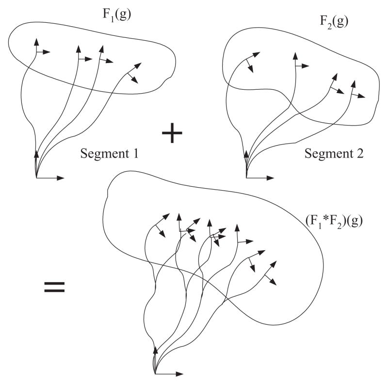
where h, g ∈ SE(3). The geometric meaning of this convolution is that the second function is swept and weighted by the first. For example, if the full distribution of positions and orientations of two adjacent segments of a polymer chain are known (see Fig. 1), then the concatenation of the segments yields a chain with distribution F1 * F2. Note that generally the order of concatenation matters for inhomogeneous chains and F1 * F2 ≠ F2 * F1 if F1 ≠ F2. This convolution of functions on the group can be calculated by direct sequential products of Fourier transform of each function as
Fig. 1.
Pictorial explanation of the concept of convolution. The second function is swept and weighted by the first. If the full distribution of positions and orientations of two adjacent segments of a polymer chain, F1 and F2, are known, then the concatenation of the segments yields a chain with distribution F1 * F2.
| (12) |
Note that unlike the case of the classical convolution theorem the order of multiplication matters.
2.2 PDF of end-to-end distance
In this section, we derive the probability density function of end-to-end distance for discrete-link polymer models using the Fourier transform obtained in the previous section. The PDF of end-to-end distance, denoted as f(r), is, in fact, a marginal 1-D PDF of the 6-D PDF of relative end-to-end position and orientation, denoted as F(g) where g = (r, R) ∈ SE(3). The final form of the result to be derived can be found in the literature [13,22,23]. However, since those do not contain detailed derivations, we derive it in this section.
The inverse Fourier transform of F̂ can be obtained using Eqs. (9) or (10). To obtain the probability density function of end-to-end distance, let us first consider the integral over SO(3) of F(g)
| (13) |
If we separate and write for the last integral, then it becomes
where . In order for this integral to have non-zero value, one can easily find that j = 0, and m = 0. The integral on β, then simply becomes
Here we use the relation , where Pl is the lth Legendre polynomial, and substitute cosβ into x. The integral of each Legendre polynomial becomes zero when l ≠ 0. Hence we find the condition that l = 0. Looking at the range of summation, one can also find that s = 0 should be satisfied. Therefore Eq. (13) can be expressed in a compact form as
| (14) |
If we integrate Eq. (14) over the surface of a unit sphere and multiply by r2, then the result will be the probability density function of end-to-end distance. Let that probability density function be denoted as f(r), then it is of the form
| (15) |
Since [l′, m′|p, 0|0, 0](r) consists of such functions as eimφ and Pl′(cosθ) due to the fact that l = m = s = 0, one can easily find that l′ = m′ = 0 by the similar reasoning with that given previously. Finally, we can get the end-to-end distribution as
| (16) |
Here we use the equality [13].
3 Probability Density Function of end-to-end distance
As mentioned earlier, we examine discrete-chain polymer models. In this section we derive the probability density function of end-to-end distance for three different discrete-chain polymer models.
3.1 The freely-rotating model
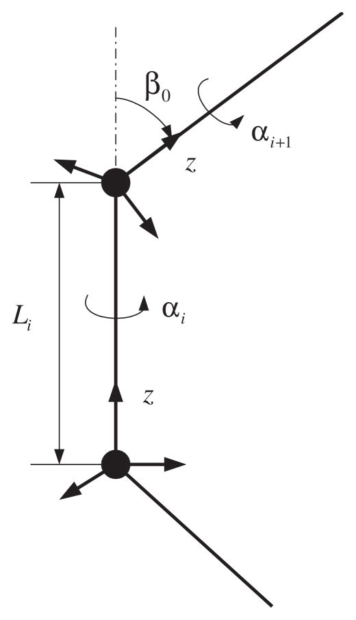
Let us assume the geometry shown in Fig. 2. Fig. 2 shows a schematic diagram of the ith link. In that figure, Li corresponds to the length of the ith bond, αi is the ith dihedral or torsional angle, and β0 is the ith bond angle. Here we use the convention that the local z axis coincides with each bond. Then the position of the distal end with respect to the proximal end can be described by means of spherical coordinates, r = [r cos φ sin θ, r sin φ sin θ, r cos θ]T. In this case, r = Li, and θ = 0. Torsional and bond angles are related to the rotation matrix of the distal end of link i with respect to its own proximal end, and can be described using by ZXZ Euler angles RZXZ(α, β, γ), in which case α = αi, β = β0, and γ = 0.
Fig. 2.
Schematic diagram of one link. Reference frame is attached so that the local z axis coincides with each link. αi is the ith torsional angle, and β0 is the ith bond angle. These are described using ZXZ Euler angles.
According to the geometry shown, one can find that the appropriate form of the probability density function for this single link can be described using Dirac delta functions. If we express it explicitly, it is of the form
| (17) |
Here, since the position of the distal end has the singularity associated with spherical coordinates (θ = 0), the φ value does not appear in the above equation. Instead, the effect of integration with respect to φ is included in the constant, so that consequently, the constant term contains 4π/r2sinθ [13]. As for the α angle, which corresponds to the ith torsional angle αi of a polymer, we assume that rotation around this angle to be uniformly distributed, so that probability of those angles are . This assumption makes it the freely-rotating chain model. Then we can take the SE(3)-Fourier transform for the function in Eq. (17) by using Eq. (8). From [13], one sees that
With the above expression, Eq. (1), the properties of Dirac delta function, and the fact that has non-zero value only when m = 0, we can derive the probability density function of the ith link as
| (18) |
where r0 means the position vector of distal end with respect to the reference frame attached to the proximal end. In component form, it can be written as
| (19) |
only when m = 0. Otherwise, it is zero.
Since we get the Fourier transform of the probability density function of the ith link derived above, now we can obtain the Fourier transform of an N-link polymer by utilizing the generalized convolution on SE(3), which is simply expressed in Eq. (12). Let us denote the Fourier transform of an N-link polymer as F̂. This can be obtained simply by multiplying each Fourier transform in reversed order as
| (20) |
when we apply the above arguments to obtain the end-to-end distance distribution. Since we only need to consider the case when s = 0, Eq. (19) can be further simplified to the following form
| (21) |
only when m = 0. Otherwise, becomes zero. In the above equation, the Clebsch-Gordan coefficient can be calculated by the following simple formula [39]
when a+b+c = 2g, where g is a positive integer. When a+b+c = 2g +1, the corresponding Clebsch-Gordan coefficients have zero values. Then by utilizing Eqs. (20) and (16), we can obtain the probability density function of end-to-end distance for the N-link polymer chain.
3.2 The independent energy model
In this model, the potential energy is expressed as
. With this in mind, we define the PDF of the ith link as
| (22) |
where g = (r, R(α, β, γ)) ∈ SE(3) and the partition function Z is defined as . The Fourier transform of this function becomes
| (23) |
Using the fact that vanishes except when j = −m, |m| ≤ l′, Eq. (23) is further simplified to the following form
| (24) |
only when |m| ≤ l′. If not, the above Fourier transform becomes zero. After that, by using Eqs. (20) and (16) we can obtain the end-to-end distance distribution.
3.3 The interdependent pairwise energy model
As we did in the freely-rotating model and in the independent energy model, let us assume the geometry shown in Fig. 2. The difference now is that
| (25) |
First, we define the following. Let d(g−α) be , and ∫SE(3)−α = ∫γ∫β∫θ∫φ∫r, i.e., only ∫α(·)dα is missing in the integration and measure. We also define . Then referring to [13], we can define
| (26) |
By the same analogy as in the previous case, due to the fact that the integral has non-zero value only when j = −m only for |m| ≤ l′, it becomes
| (27) |
Now, let us consider the Boltzmann-weighted convolution of the ith and i+1st links of the form
| (28) |
If we take the SE(3)-Fourier Transform of the convolution, then it is written as
| (29) |
Here we use g′ = h−1 ◦ g, dg′ = dg, Us(g′−1 ◦ h−1) = Us(g′−1)Us(h−1), and . By means of Eqs. (26) and (27), Eq. (29) can be written in the compact form
| (30) |
Suppose that there are N links, and let the number density of the distal end be numF, then the Fourier Transform gives
| (31) |
where α = (α1, ···, αN) and . Then the Fourier Transform of the PDF can be obtained by normalization as
| (32) |
where the partition function Z is defined as
| (33) |
Now, we employ a similar method as in [13,35]. First, let us define for i + 1 < l − 1
| (34) |
Then, for example assuming that we divide the total chain into two segments (α0, ···, αi) and (αi+1, ···, αN), the Fourier Transform of the number density numF becomes
| (35) |
In practice, we can break the whole chain apart into segments with 2 or 3 monomers. More specifically, let us define
| (36) |
Then Eq. (34) becomes
| (37) |
and we can apply this equation sequentially to reach Eq. (35). After that, we can apply the same normalization as in Eq. (32). Then the end-to-end distance distribution f(r) can be calculated from Eq. (16).
Note that, in order to obtain the partition function Z, we can apply the same method described above. Specifically, if we use 1 instead of and in Eq. (36), then the convolution-like function eventually gives the partition function.
4 Efficient Implementation
In numerical work, computational cost is often a critical issue. In this section, we mention efficient methods for calculating the end-to-end distribution with the proposed method.
Among the three different models presented in this paper, the computational speed for the freely rotating and the independent energy model cases is faster than that of the interdependent energy model. We can store the Fourier transform of each link in advance as functions of the frequency factor p, then can apply Eq. (12) to obtain the end-to-end distribution of a given polymer. This process is nothing more than matrix multiplication.
However, when it comes to the interdependent energy model case, the situation is not as simple as the two other cases. As one can see from Eq. (37), one needs double integration at each step. For example, assume that we divide one torsion angle into n cells. Then the number of points in each αi becomes n +1. Each process of matrix multiplication and summation in Eq. (37) needs O(n4) computations. The main problem is that if we use n = 50 or greater than that (n = 100, for example), which is required in most cases because one needs a large value of n to avoid aliasing effects in the Fourier transform, then O(n4) is really a huge number, which means that the direct implementation of Eq. (37) is not an efficient way to implement the method for the interdependent energy model case. For this reason, we present more efficient ways of implementing the interdependent energy model.
First, we compute the Fourier series of ui,i+1(αi, αi+1) = e−Ei,i+1(αi,αi+1)/kBT. Then it becomes
| (38) |
In practice, if we use a band width, B, for approximating the exponential of the energy function, then we can utilize the exponential of the energy function as
| (39) |
Here the Fourier coefficient i,i+1ûm,n is defined as
Also a closer investigation of Eq. (27) gives
| (40) |
where
| (41) |
for |m| ≤ l′. Otherwise it becomes zero. If we express it in matrix form, it becomes
| (42) |
where means the diagonal matrix whose diagonal element is eimαi. Let us assume that there are 8 links in a given segment of polymer. We can construct the following by means of Eqs. (36) and (39)
| (43) |
Similarly, we can construct for the 3rd and 4th links as
| (44) |
Then can be expressed, by Eq. (42), as
| (45) |
where each mi represents the index in Eq. (42) for the ith link. Due to the fact that the integral has non-zero value only when m = 0, this can be simplified further to the following form
| (46) |
where
| (47) |
where δj,k is a Kronecker delta. Here 1,2ûj1,k1, 3,4ûj2,k2, and 2,3ûj,k represent the Fourier coefficients for E1,2(α1, α2), E3,4(α3, α4), and E2,3(α2, α3), respectively. Similarly,
| (48) |
With Eqs. (46) and (48), we can obtain the following
| (49) |
where
| (50) |
Here 4,5ûj,k is the Fourier coefficient for E4,5(α4, α5). If there are more than 8 links, then one can repeat Eqs. (49) and (50) to obtain where N is the number of links. At the final step, we can obtain numF̂s by
| (51) |
The partition function Z can be calculated similarly with all ’s replaced by 1 in the above procedure.
The above approach has an advantage compared to the direct double integration in that we do not need to perform integration. Instead, we can only select the set of indices which makes the integration of eimα part nonzero. Then, the total computational cost for each summation and matrix multiplication processes becomes O(B4 × a2), where the maximum value of a is O(B). In practice, the number of B as 4 ~ 7 can give a good approximation of the exponential of energy function. Another issue is that, since ui,i+1(αi, αi+1) is already expressed in terms of harmonics, we do not need a large value of Nb, which is the band width in the Fourier transform for SE(3), compared with the case where the original energy function is used. Since the computational cost also depends on the size of Fourier transform matrix for SE(3), one can find that the approach presented in this section is much faster than direct double integration approach.
5 Application to Polypeptide Chains
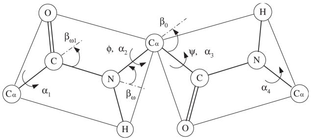
We can also apply our proposed method to polypeptide chains. Polypeptide chains have interesting features compared with other general chains, such as polyethylene, etc. We depict the diagram of polypeptide chain structure in Fig. 3. First, the torsion angle around the C–N bond is nearly fixed to be 180°. The torsion angle between Cα and C is called ψ angle, and that between N and Cα is called φ angle. The allowable range of values for the angle pair (ψ, φ) is obtained from the Ramachandran plot [40]. This also shows that the behavior of a polypeptide chain can be described using interdependent pairwise energy model. In fact, this is already known as “the Flory isolated-pair hypothesis” [1,41]. Although it turns out that this isolated-pair hypothesis requires some modification [41], it still serves as a good approximation to describe the behavior of polypeptide chains. In this section, we apply our proposed method to obtain end-to-end distance distribution of polypeptide chain models defined by the Ramachandran plot.
Fig. 3.
Schematic diagram of a polypeptide chain. The torsion angle of the C–N bond is nearly fixed as 180°. In numerical examples, βω and βω1 are assumed 63.8° and 58.3°, respectively.
Looking at Fig. 3, as mentioned earlier, unlike other polymers such as polyethylene, etc., the C–N bond does not have energy interaction with two adjacent bonds, Cα–C and N–Cα. Let the probability density function of the C–N bond be ωF. If the torsional angle along the C–N bond is 180°, or π radians, then ωF becomes
| (52) |
where βω and Lω are bond angle and bond length of C–N bond, respectively. Here the ω angle is assumed to be 180° or π radians. The Fourier Transform for SE(3) gives
| (53) |
for |m| ≤ l′. Otherwise, this becomes zero. One can, then, define the following together with Eq. (26)
| (54) |
Then we can apply the method in the previous section to this polypeptide chain model. Note that the polypeptide chain case has much simpler form than general polymer chains due to the fact that
| (55) |
That is, each pairwise energy becomes independent. Hence, we can use an energy function with the following form
| (56) |
where
| (57) |
First we consider 8 residues among the polypeptide chain consisting of N residues. For convenience, let us assume that N has the form of 2k where k is a positive integer greater than 3. We can construct the pairwise Fourier Transform-like matrices as
| (58) |
for i = 1, 3. Then
| (59) |
where
| (60) |
We can do similarly with the subchain consisting of residues 5 to 8 as
| (61) |
Then
| (62) |
where
| (63) |
After that, we can repeat until N links are reached. Finally we can obtain the Fourier Transform of end-to-end distance probability density function F(g) as
| (64) |
Here 4π2 in the first line is a normalization factor. Because all u(αi, αi+1) are normalized according to Eq. (56), the integration about the final two angles αN and α1 requires a normalization factor, which becomes ∫αN ∫α1 dα1dαN = 4π2
6 Numerical Examples
In this section three kinds of examples are demonstrated: the freely-rotating chain, the independent energy chain, and the interdependent pairwise energy chain.
6.1 The freely-rotating and the independent energy chain model
First let us take an example for the freely-rotating model. In order to verify our model, we utilize well-known formulas for the freely rotating chain model [1]. According to the Flory’s theory [1], when all the link lengths are the same and denoted as L, and all the bond angles have the same values as θ, then the average of the square of the end-to-end distance for the N-link polymer chain can be calculated as[1,13]
| (65) |
where α = cosθ. If we further normalize the end-to-end distance with the total chain length (divide Eq. (65) by N2L2), the equation becomes
| (66) |
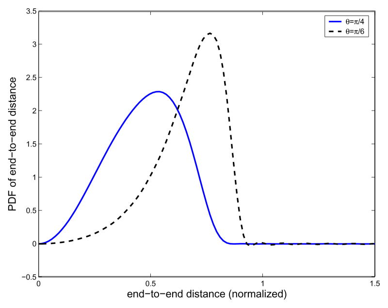
In Fig. 4 are shown the resulting end-to-end distance probability density functions for two different cases. Here the number of links in the polymer chain is fixed to be 20. If we calculate the area under the curves, it gives 1.0000, which means that the obtained curves truly represent the probability density functions. In Table 1 are shown the squares of the end-to-end distance. One can see that the corresponding results are in excellent agreement with those from Eq. (66). In the simulations, as the band width for Fourier transform for SE(3) and upper limit of integration with respect to frequency factor p, denoted as Nb and Lp respectively, Nb = 12 and Lp = 50 are used in the case of θ= π/4, and Nb = 16 and Lp = 60 are used in the case of θ = π/6.
Fig. 4.
Plot of the resulting end-to-end distance probability density functions for the freely-rotating model. The number of links is set to be 20. θ denotes the bond angle of the polymer chain. The continuous line corresponds to the case when θ= π/4, and the dotted line to the case when θ = π/6. In the simulations, the band width of the Fourier transform for SE(3) and upper limit of integration with respect to frequency factor p are denoted as Nb and Lp, respectively, and Nb = 12 and Lp = 50 are used in the case of θ = π/4, and Nb = 16 and Lp = 60 are used in the case of θ = π/6.
Table 1.
The comparison of the mean squares of the end-to-end distance.
| θ | from our model | from Eq. (66) |
|---|---|---|
| π/4 | 0.2502 | 0.2502 |
| π/6 | 0.4687 | 0.4688 |
As for the next example, we consider the following potential energy
| (67) |
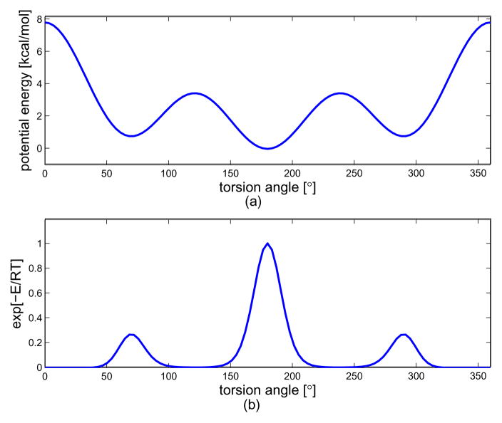
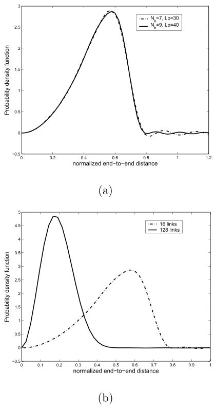
in units of kJ/mol, which is the torsional potential energy for n-Butane.[3] In Fig. 5 is shown the torsional potential energy and exponential of the potential energy. This potential energy has three minima, gauche+ (near α = 60°), trans (near α = 180°), and gauche− (near α = 300°). This expression is one general form of torsional potential energy which appears in many of polymer chains. In Fig. 6 is shown the resulting probability density function of end-to-end distance for this independent energy model. Looking at part (a), which is the case of the number of links being 16, one can see that the PDF is described more accurately as the band width for Fourier transform for SE(3), Nb, and the upper limit for the integration with respect to the frequency factor p, Lp, get larger. Especially, Nb = 7 appears to be sufficient for describing the ‘mountain’ part of the PDF, but in order for the better ‘tail’ description, we need larger Lp such as 40 in that figure. In part (b), we show the PDFs for two different numbers of links. As one can expect, when the number of links is 128, the resulting end-to-end distance distribution becomes more concentrated toward the left side.
Fig. 5.
The plot of torsional potential energy and its exponential used in the example of the independent energy model. (a) the torsional potential energy, (b) exponential of the torsional potential energy.
Fig. 6.
Plot of the resulting end-to-end distance probability density functions for the independent energy model. All the monomer chains are assumed to be identical, with β0 = 75.1°. (a) The plot of PDFs with different Nb and Lp. It shows that as Nb and Lp get larger, one can describe the corresponding PDF better. (b) The plot of PDFs with different number of links. From this figure, one can see that the PDF for chains with a large number of links gets more concentrated on the left side.
6.2 The interdependent pairwise energy chain model
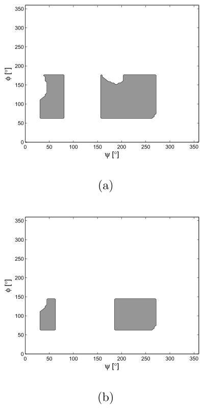
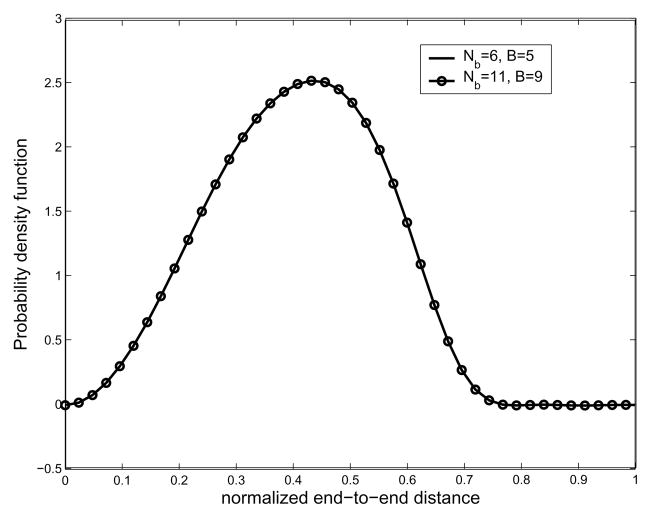
We now demonstrate the interdependent pairwise energy model case. Among various polymers, from natural to artificial ones, polypeptide chains are of special interest these days. Hence we take polypeptides as examples of the interdependent pairwise energy model. In order to generate end-to-end distance distributions, we need a 2-D energy map. One can find a way to compute the energy map from first principles using Lennard-Jones potentials [1], or using MD simulations [42]. In general, MD simulation can be trusted more than just using Lennard-Jones potentials. However, in this paper, we generate Ramachandran-like plots as a probability distribution of torsional energy. The purpose of this example is to show that the proposed method can generate end-to-end distance distributions for any type of pairwise energy function, which justifies the usage of Ramachandran-like plots. We also utilize the simplified geometric model for a polypeptide chain based on the same reason above. All the information about bond angles and bond lengths of peptide units are borrowed from [41]. The hard-sphere contact distances are also borrowed from [41]. As for hard-sphere radius for residues (alanine and valine), we treat CH3 to be approximately of the same size as C, from the fact that, according to [1], the radius of CH2 are greater than that of C by only 0.15 Å. Fig. 7 shows the Ramachandran-like plot for each dipeptide, alanine and valine. We treat these maps as the exponential of the torsional potential energy, e−Ei,i+1(αi,αi+1)/kBT and the height of each allowed (gray) region is set at 2. In Fig. 8 is shown the resulting end-to-end distance PDF for a polyalanine chain with 16 residues.
Fig. 7.
The Ramachandran-like plots of approximate models for dipeptide used in the numerical examples. (a) Alanine dipeptide. (b) Valine dipeptide. Gray represents allowed regions.
Fig. 8.
Plot of the resulting end-to-end distance probability density functions for the interdependent energy model. This corresponds to the case of a poly-alanine chain. The number of links is 16 in both cases. It shows that lower value of Nb and B is good enough to describe the corresponding PDF of the end-to-end distance.
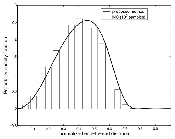
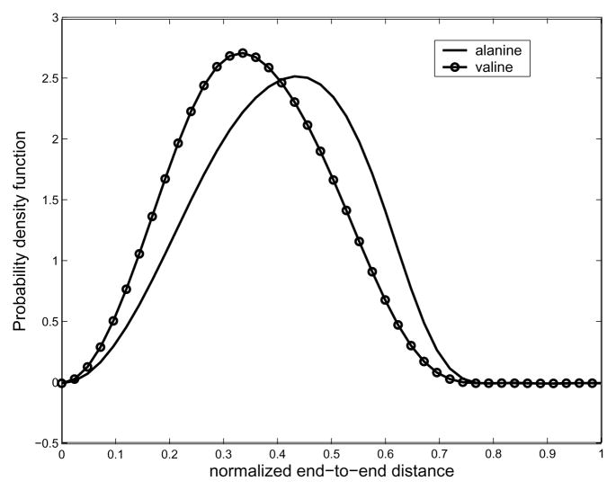
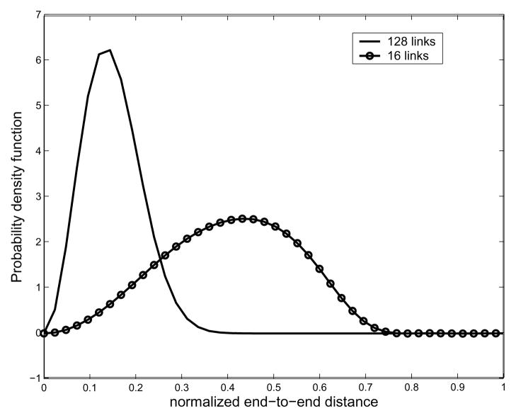
As mentioned earlier, the small value of bandwidth B, which is for the classical Fourier series approximation of the exponential of the torsional potential energy, is good enough for describing the corresponding PDF, and so is the bandwidth Nb for Fourier transform matrix for SE(3). In order to verify our method, we performed MC simulation for polyalanine with 16 residues. In the MC sampling, since the probabilities within the allowable region are the same, we randomly select a set of pairs of φ, ψ angles to generate as many conformations of a polyalanine chain as possible given computing/time constraints. In practice, we generate 106 conformations to generate the histogram of the end-to-end distance. In Fig. 9 is shown pairwise energy model. In order to generate end-to-end distance distributions, we need a 2D energy map. One can find a way to compute the energy map from first principles using Lennard-Jones potentials [1], or using MD simulations [42]. In general, MD simulation can be trusted more than just using LennardJones potentials. However, in this paper, we generate Ramachandran-like plots as a probability distribution of torsional energy. The purpose of this example is to show that the proposed method can generate end-to-end distance distributions for any type of pairwise energy function, which justifies the usage of Ramachandran-like plots. We also utilize the simplified geometric model for a polypeptide chain based on the same reason above. All the information about bond angles and bond lengths of peptide units are borrowed from [41]. The hard-sphere contact distances are also borrowed from [41]. As for hard-sphere radius for residues (alanine and valine), we treat CH3 to be approximately of the same size the comparison between the result from MC simulation and that from our method. One can observe good agreement between both the results, though MC is not able to give the exact PDF in this situation. We believe this happens for two reasons: first, the conformational space is too large to allow for sufficient sampling; and second, random number generators in software packages (in this case Matlab) are not truly random, and this lack of true randomness becomes noticable as the number of samples becomes very large. Also in Fig. 10 one can see that the PDFs corresponding to different energy becomes different. Looking at Fig. 11, which shows the resulting end-to-end distance PDF for polyalanine chains with different number of links, one can also see that when the number of links is 128, the resulting end-to-end distance distribution becomes more concentrated toward the left side.
Fig. 9.
Comparison of the result from the proposed method with MC sampling. In MC sampling, 106 conformations are randomly selected to generate histogram which is equivalent to PDF of the end-to-end distance. Both the cases correspond to polyalanine with 16 residues.
Fig. 10.
Comparison of two different polypeptides with the same number of links. In this figure, the number of links is set to be 16.
Fig. 11.
Plot of the resulting end-to-end distance probability density functions for the polyalanine chain for different number of links. As one can see, the larger the number of links, the more concentrated to the left side the resulting plot becomes.
6.3 The comparison with other chain models
In this section, we demonstrate the comparison between the end-to-end distance distribution from other chain models distribution and that from the proposed method.
One can find the formula of the spatial distribution for the Gaussian chain model and the freely-joint chain model in [1,3]. Following the notation in [1], the end-to-end distribution for the Gaussian chain is expressed as
| (68) |
and for the N-link freely-joint chain model
| (69) |
where r denotes the end-to-end vector and r denotes the end-to-end distance. <r2> corresponds to the mean square of the end-to-end distance. From these functions, one can obtain the PDFs of the end-to-end distance as
| (70) |
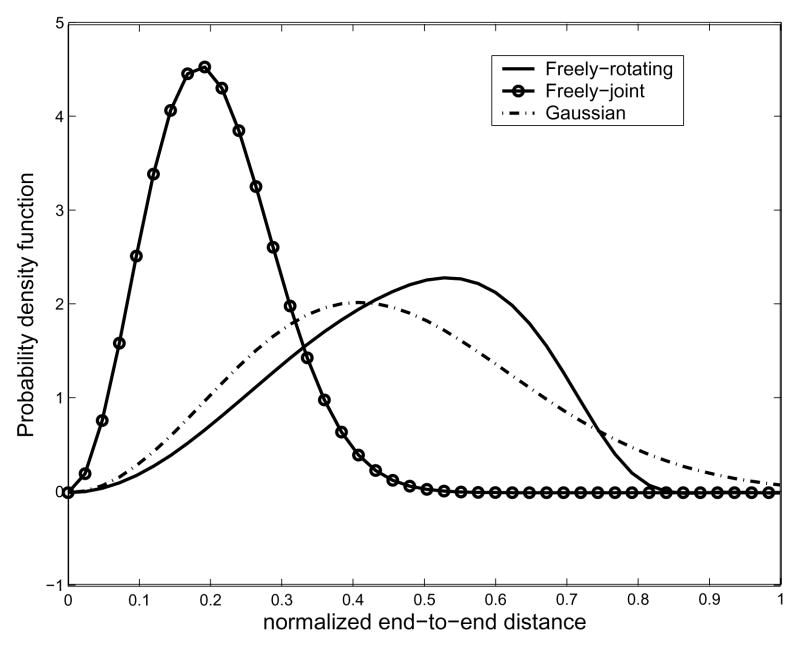
First we compare the freely-joint chain model and the Gaussian chain model with the freely-rotating chain model from the proposed method. In this example, the number of links is 20 and the bond angle for the freely-rotating chain model is π/4. Referring to Table 1, we find that <r2>= 0.2502. In Fig. 12, we show the result of comparison among these three different models. As one can see, different chain model generates different PDF of the end-to-end distance when the length of a chain is relatively short.
Fig. 12.
Comparison among the Gaussian chain, the freely-joint chain, and the freely-rotating chain model. The number of links is set to be 20. As one can see, the resulting PDFs are different according to each model.
Next, we compare the Gaussian chain model with our examples in previous sections. That is to say, we take the freely-rotating chain model, the independent energy chain model, and the interdependent pairwise energy chain model to compare with the Gaussian chain model when the length of a chain is large. Particularly, in this example we take the number of links is 128 and the bond angle is π/4 for the freely-rotating chain model. As for independent energy chain model, we utilize the same example in the first subsection. Also we take the polyalanine chain in the second subsection as an example of the interdependent pairwise energy chain model. As for the Gaussian chain model, we first compute <r2> from the results of the proposed method, and then obtain the Gaussian chain distribution from Eqs. (68) and (70). In Fig. 13 we show the results of comparison between each of the three different chain models and the Gaussian chain model. As one can see, these figures verify that all classical linear chain models behave as the Gaussian chain as the length of a chain becomes very large.
Fig. 13.
(a) Comparison between the Gaussian chain and the freely-rotating chain model. (b) Comparison between the independent energy chain model and the Gaussian chain model. (c) Comparison between the interdependent pairwise energy chain model (polyalanine) and the Gaussian chain model. In all cases, the number of links is set to be 128. It shows that when the length of polymer chain is very long, then the freely-rotating chain model, the independent energy chain model, and the interdependent pairwise energy chain model all become the same as the Gaussian chain.
7 Conclusions
In this paper, we have presented a unified method to generate the probability density function of the end-to-end distance for discrete-chain polymer models. Our method is based on previous work which utilizes the generalized convolution and extends it by employing the Fourier transform for SE(3). The proposed method is general enough to be applied to any of classical polymer chain models. We have formulated the proposed method for three different discrete polymer chain models: the freely-rotating model, the independent torsional energy model, and interdependent pairwise energy model. We have also developed efficient implementation method, particularly for the interdependent pairwise energy model, by approximating the exponential of the torsional potential function with the classical Fourier series. We have demonstrated the versatility of the proposed method by numerical examples. We expect that this method, which can generate both one-dimensional marginal PDFs and multi-dimensional PDFs (e.g., PDF for end-to-end distance and orientation of the distal end of a polymer chain), can be useful in a wider range of conformational studies on polymer chains, including artificial polymer chains and natural ones such as polypeptide and single-stranded RNA molecules.
Acknowledgments
This work was performed under NIH Grant R01GM075310.
Contributor Information
Jin Seob Kim, Email: jkim115@jhu.edu.
Gregory S. Chirikjian, Email: gregc@jhu.edu.
References
- 1.Flory PJ. Statistical mechanics of chain molecules. New York: Wiley-Interscience; 1969. [Google Scholar]
- 2.Dill KA. Protein Sci. 1999;8:1166. doi: 10.1110/ps.8.6.1166. [DOI] [PMC free article] [PubMed] [Google Scholar]
- 3.Mattice WL, Suter UW. Conformational theory of large molecules. New York: Wiley; 1994. [Google Scholar]
- 4.Lapidus LJ, Steinbach PJ, Eaton WA, Szabo A, Hofrichter J. J Phys Chem B. 2002;106:11628. [Google Scholar]
- 5.Cannavacciuolo L, Pedersen JS. J Chem Phys. 2004;120:8862. doi: 10.1063/1.1691392. [DOI] [PubMed] [Google Scholar]
- 6.Winkler RG. J Chem Phys. 2003;118:2919. [Google Scholar]
- 7.Samuel J, Sinha S. Phys Rev E 050801 [Google Scholar]
- 8.Mark JE, Curro JG. J Chem Phys. 1983;79:5705. [Google Scholar]
- 9.Curro JG, Mark JE. J Chem Phys. 1984;80:4521. [Google Scholar]
- 10.Yuan W, Kloczkowski A, Mark JE, Sharaf MA. J Polym Sci, Part B: Polym Phys. 1996;34:1647. [Google Scholar]
- 11.Sharaf MA, Mark JE. Polymer. 2002;43:643. [Google Scholar]
- 12.Sharaf MA, Mark JE. Polymer. 2004;45:3943. [Google Scholar]
- 13.Chirikjian GS, Kyatkin AB. Engineering applications of noncommutative harmonic analysis. New York: CRC Press; 2001. [Google Scholar]
- 14.Marko JF, Siggia ED. Macromolecules. 1994;27:981. [Google Scholar]
- 15.Haijin Z, Zhong-Can O. Phys Rev E. 1998;58:4816. [Google Scholar]
- 16.des Cloizeaux J, Jannink G. Polymers in solution: their modelling and structure. Oxford: Clarendon Press; 1990. [Google Scholar]
- 17.Yamakawa H. Helical wormlike chains in polymer solutions. Berlin: Springer; 1997. [Google Scholar]
- 18.Hamprecht B, Janke W, Kleinert H. Phys Lett A. 2004;330:254. [Google Scholar]
- 19.Bhattacharjee JK, Thirumalai D, Bryngelson JD. cond-mat/9705200. [Google Scholar]
- 20.Stepanow S, Schütz M. Europhys Lett. 2002;60:546. [Google Scholar]
- 21.Zhou H. J Phys Chem B. 2001;105:6763. [Google Scholar]
- 22.Chirikjian GS, Wang Y. Phys Rev E. 2000;62:880. doi: 10.1103/physreve.62.880. [DOI] [PubMed] [Google Scholar]
- 23.Zhou Y, Chirikjian GS. J Chem Phys. 2003;119:4962. [Google Scholar]
- 24.Kostrowicki J, Scheraga HA. Comput Polym Sci. 1995;5:47. [Google Scholar]
- 25.Freire JJ, Rodrigo MM. J Chem Phys. 1980;72:6376. [Google Scholar]
- 26.Freire J, Fixman M. J Chem Phys. 1978;69:634. [Google Scholar]
- 27.Fixman M, Skolnick J. J Chem Phys. 1976;65:1700. [Google Scholar]
- 28.Fixman M. J Chem Phys. 1973;58:1559. [Google Scholar]
- 29.Rubio AM, Freire JJ. Macromolecules. 1989;22:333. [Google Scholar]
- 30.He S, Scheraga HA. J Chem Phys. 1998;108:271. [Google Scholar]
- 31.Plimpton S, Hendrickson B. J Comput Chem. 1996;17:326. [Google Scholar]
- 32.Lyulin AV, Dünweg B, Borisov OV, Darinskii AA. Macromolecules. 1999;32:3264. [Google Scholar]
- 33.Kloczkowski A, Sen TZ, Sharaf MA. Polymer. 2005;46:4373. [Google Scholar]
- 34.Marcelo G, Tarazona MP, Saiz E. Polymer. 2004;45:1321. [Google Scholar]
- 35.Chirikjian GS. Comput Theor Polym Sci. 2001;11:143. [Google Scholar]
- 36.Miller W. Commun Pure Appl Math. 1964;17:527. [Google Scholar]
- 37.Vilenkin NJ, Klimyk AU. Representation of Lie groups and special function. Vol. 1. Dordrecht: Kluwer Academic; 1991. [Google Scholar]
- 38.Gelfand IM, Minlos RA, Shapiro ZY. Representations of the rotation and Lorentz groups and their applications. New York: Macmillan; 1963. [Google Scholar]
- 39.Varshalovich NJ, Moskalev AN, Khersonskii VK. Quantum theory of angular momentum. NJ: World Scientific Publishing; 1988. [Google Scholar]
- 40.Branden C, Tooze J. Introduction to protein structure. 2. New York: Garland Publishing; 1999. [Google Scholar]
- 41.Pappu RV, Srinivasan R, Rose GD. Proc Natl Acad Sci. 2000;97:12565. doi: 10.1073/pnas.97.23.12565. [DOI] [PMC free article] [PubMed] [Google Scholar]
- 42.Bahar I, Zuniga I, Dodge R, Mattice WL. Macromolecules. 1991;24:2986. [Google Scholar]


