Staggered Mesh Ewald: An extension of the Smooth Particle-Mesh Ewald method adding great versatility

Abstract

We draw on an old technique for improving the accuracy of mesh-based field calculations to extend the popular Smooth Particle Mesh Ewald (SPME) algorithm as the Staggered Mesh Ewald (StME) algorithm. StME improves the accuracy of computed forces by up to 1.2 orders of magnitude and also reduces the drift in system momentum inherent in the SPME method by averaging the results of two separate reciprocal space calculations. StME can use charge mesh spacings roughly 1.5× larger than SPME to obtain comparable levels of accuracy; the one mesh in an SPME calculation can therefore be replaced with two separate meshes, each less than one third of the original size. Coarsening the charge mesh can be balanced with reductions in the direct space cutoff to optimize performance: the efficiency of StME rivals or exceeds that of SPME calculations with similarly optimized parameters. StME may also offer advantages for parallel molecular dynamics simulations because it permits the use of coarser meshes without requiring higher orders of charge interpolation and also because the two reciprocal space calculations can be run independently if that is most suitable for the machine architecture. We are planning other improvements to the standard SPME algorithm, and anticipate that StME will work synergistically will all of them to dramatically improve the efficiency and parallel scaling of molecular simulations.

1 Introduction

With few exceptions,^1,2 the method of choice for computing long-ranged electrostatic interactions in molecular simulations with periodic boundary conditions is the Ewald sum.³ Whereas simple truncation of long-ranged electrostatic interactions has been shown to give rise to significant simulation artifacts,^4,5 the use of modern Ewald algorithms enables more efficient simulations with effectively no omission of long-ranged electrostatic interactions.

In its original formulation, the Ewald sum for a system of N particles was an O(N²) computation, but the introduction of particle:mesh methods have reduced the complexity to O(NlogN)^6,7,8 and even to O(N),^9,10,11 at which point the choice of optimal algorithm falls to the computational constants of the various methods given the problem’s size and particle density. Most concisely, particle:mesh methods rephrase the problem of computing the electrostatic potential of a system of point (or otherwise highly localized) charges from solving O(N²) pairwise interactions to solving Poisson’s equation for a highly smoothed version of the system’s charges and then determining the difference between this smoothed-charge potential and the system’s actual point charge density. This approach can be efficient because the smoothed charge density is written as a Gaussian convolution of the point charge density: the interaction of two Gaussian charges rapidly converges to the interaction of two point charges at distances greater than about six times the Gaussian’s root-mean-squared deviation. The mesh-based electrostatic potential can then be solved by fast Fourier transforms (FFTs) in O(N logN) operations or by a finite-difference Poisson solver in O(N) operations, while the modification needed to recover the point-charge potential is computed in O(N) operations, similar to a simple truncation method.

Molecular simulations require accurate force calculations as well as values of the total system energy. In the primary publications of the many available electrostatic mesh methods^10,8,12,7 there have been analyses of the parameters such as the width of the Gaussian charge smoothing function, direct space truncation length, and mesh density required to obtain a given degree of accuracy in forces acting on each atom or the total system energy. In simulations, the goal is to balance these parameters to maximize efficiency. Mostly, this is a matter of minimizing the total computational effort, but with the availability of highly scalable molecular dynamics codes,^13,2,14,15 another critical factor in the computational efficiency of an algorithm is the communications requirement. Parallel implementations on many different machine architectures can therefore benefit from algorithms that can obtain a given level of accuracy with the widest possible range of parameters.

In this communication, we draw upon a technique used in the 1970s for improving the accuracy of force calculations in particle:mesh methods. The method, known then as “interlacing,” was first applied to plasma simulations by Chen and colleagues¹⁶ and later to molecular simulations by Eastwood.¹⁷ The fundamental improvement is to use two or more meshes staggered such that their points are displaced by some fraction of the mesh spacing—typically 1/2. Averaging the results obtained from each mesh produces significant error cancellation. When it was introduced, the method was viewed as a means for achieving higher levels of accuracy with limited amounts of computer memory, at the expense of speed. After re-discovering the method, however, we observe that it improves the overall computational efficiency on modern computers and may help to improve the parallel scaling of molecular simulations. We apply interlacing to the popular Smooth Particle Mesh Ewald method, and term the extended method “Staggered Mesh Ewald.”

2 Summary of particle mesh Ewald methods

If one calculates the electrostatic potential of a periodic system of charges by applying using Coulomb’s law over all pairs of charges in a large number of images of the unit cell, the process is cumbersome and the result is only conditionally convergent. The Ewald method employs a mathematical identity to split the Coulomb sum E^(coul) into a “direct space” sum E^(dir) that converges rapidly (with a short interparticle distance |r_ij|) in real or “direct” space, and a “reciprocal space” E^(rec) sum that converges absolutely in “reciprocal” space after Fourier transformation.

$$\begin{array}{c}{E}^{\left(\mathrm{coul}\right)}=\frac{1}{2}\sum _{\mathrm{n}}\sum _i\sum _{j\ne i}\frac{k_c{q}_i{q}_j}{\left|\mathbf{n}\cdot \mathbf{L}+{\mathbf{r}}_{\mathit{ij}}\right|}\\ E^{\left(\mathrm{dir}\right)}\simeq \frac{1}{2}\sum _i\sum _{j\ne i}\frac{k_c{q}_i{q}_j\left(1-\mathrm{erf}\left(\beta \left|\mathbf{r}\right|\right)\right)}{\left|{\mathbf{r}}_{\mathit{ij}}\right|}\\ E^{\left(\mathrm{rec}\right)}=\frac{1}{2}\sum _{\mathrm{n}}\sum _i\sum _{j\ne i}\frac{k_c{q}_i{q}_j\mathrm{erf}\left(\beta \left|\mathbf{r}\right|\right)}{\left|\mathbf{n}\cdot \mathbf{L}+{\mathbf{r}}_{\mathit{ij}}\right|}\end{array}$$ (1)

Above, n represents all unit cell images, including the primary unit cell, L is a 3 × 3 matrix whos columns are the unit cell lattice vectors, i and j run over all charged particles in the system, r_ij is the interparticle distance, k_c is Coulomb’s constant, and β is the “Ewald coefficient.” (Exclusions of electrostatic interactions between bonded atoms in the primary unit cell are omitted from this discussion for simplicity.) The Ewald method reduces the problem of computing the electrostatic energy (and forces on all particles) to an O(N²) problem, a double sum over all particles to obtain the reciprocal space sum. (Computing E^(dir) is an O(N) problem because interactions can be neglected beyond some direct space cutoff L_cut.)

Physically, the Ewald method is equivalent to treating the system of point (or otherwise highly localized) charges as a system of diffuse Gaussian charges, solving the electrostatic potential E^(rec) and forces ∂E^(rec)/∂r_i due to the Gaussian charge system, and then modifying those quantities with E^(dir) and ∂E^(dir)/∂r_i to recover the interactions of the point charges. Ewald mesh methods take this view of the Ewald reciprocal space procedure so that the reciprocal space sum can be solved on a mesh. (The direct space part is identical to the original Ewald method, and will not be discussed further.)

In general, the procedure with any Ewald mesh method entails four stages: 1.) interpolate the charge mesh Q given the positions of particles and the magnitudes of partial charges, 2.) smooth the interpolated point charges into Gaussian charges of the desired width, 3.) compute the electrostatic potential Φ^(rec) by solving Poisson’s equation for the smoothed charge density, and 4.) compute the electrostatic potential energy and forces given the derivatives of the charge density in Q and the potential Φ^(rec). Many Ewald mesh methods, including the Smooth Particle Mesh Ewald⁸ method that we will focus on during the results, make use of Fast Fourier Transforms (FFTs) to solve Poisson’s equation; in those cases it is convenient to combine stages 2.) and 3.). The charge mesh Q is transformed using the forward three-dimensional FFT to obtain Q̂, which is then multiplied element-wise by the transformed reciprocal space pair potential θ̂^(rec). The inverse three-dimensional FFT is then applied to the product to complete the convolution Φ^(rec) = Q ⋆ θ^(rec).

The two FFTs needed to convolute Q with θ^(rec) have O(N logN) computational complexity, much better than the complexity of the original Ewald method. However, for highly parallel molecular dynamics applications, the FFTs still require global data communication: every processor involved in the FFTs must broadcast its part of the problem to all other processors, and in turn receive similar information from every other processor. This constraint on the ultimate scalability of the calculation has driven the development of real-space methods for solving Φ^(rec).^9,10,11 However, none of these methods has become widely used on commodity hardware because they are all considerably more expensive than the FFT-based methods: the break-even point comes at very high processor counts, which even today are not widely available. The Staggered Mesh Ewald method presented in this communication offers a way to reduce the total amount of mesh data that must be transformed, which we will show can help to accelerate simulations on a single processor and may help extend the scalability of FFT-based Ewald mesh methods.

3 Summary of mesh staggering methods

Mesh staggering, or “interlacing” as it was originally termed, uses multiple samples of the interpolated charge density of particles on a mesh to suppress errors in the mesh calculation due to “aliasing.”⁷ Interpolation of a particle to a mesh creates a spectrum of aliases for that particle at each mesh point; because the spectrum is not perfectly smooth, the effects of different aliases on other aliases from the same particle or aliases of a nearby particle can be distorted by their proximity on the mesh. The most basic outcome of aliasing is the fluctuation of forces on particles as a function of their alignment relative to the mesh, which in turn is detrimental to momentum and energy conservation. By sampling multiple spectra of each particle on the mesh, different sets of aliases can be generated. Although each of these spectra contains roughly the same level of error in the interactions of each particle’s aliases, the errors from multiple spectra may cancel if the spectra evenly sample the possible alignments of the system’s particles relative to the mesh. The simplest and most economical implementation of the mesh staggering technique involves mapping particles to two meshes staggered such that points of one mesh fall exactly halfway in between those of the other.¹⁶

4 Methods

4.1 Preparation of primary test cases

Anticipating that condensed-phase molecular dynamics simulations will be the primary application of the Staggered Mesh Ewald (StME) method, we selected four test systems: a streptavidin tetramer¹⁸ solvated in a cubic cell, a condensed mixture of 35% v/v glycerol and water in a monoclinic cell, a scorpion toxin protein crystal lattice¹⁹ solvated with water and ammonium acetate in an orthorhombic noncubic cell, and a cyclooxygenase-2 (COX-2) dimer²⁰ solvated in a truncated octahedral cell. Dimensions and atom counts in all of the simulation cells are provided in Table 1. Together, these four test cases span the available types of periodic simulation cells and encompass a variety of condensed-phase systems.

Table 1. Test cases for the Staggered Mesh Ewald method.

The cases presented here span a variety of simulation cell geometries. All systems are in the condensed phase and were pre-equilibrated by molecular dynamics simulations at constant pressure.

Case	Cell Dimensions (a, b, c), Å	Cell Dimensions (α,β,γ)	Atom Count
Streptavidin	89.7 × 89.7 × 89.7	90°, 90°, 90°	73305
Protein Crystal	91.3 × 81.3 × 91.0	90°, 90°, 90°	73944
Glycerol Solution	69.7 × 69.7 × 89.0	60°, 90°, 90°	39808
Cyclooxygenase-2	114.8 × 114.8 × 114.8	109.5°, 109.5°, 109.5°	118833

The SPC/E water model was used in all cases, glycerol parameters were obtained from Chelli and coworkers,²¹ and any proteins were modeled with the AMBER FF99SB force field.²² Prior to electrostatic calculations, all systems were equilibrated with at least 650ps of molecular dynamics, including position-restrained dynamics if proteins were present and constant-pressure dynamics to reach each system’s equilibrium density.

4.2 Accuracy standards for Ewald calculations

To compare different Ewald methods, it is necessary to define what parameters determine the accuracy of the calculation and also what is an “acceptable” level of accuracy. We will summarize these parameters here and then assess the efficiency of Ewald methods in terms of acceptable combinations of the parameters in the Results.

The accuracy of the direct space part of any Ewald electrostatics calculation is determined by the direct sum tolerance D_tol. Briefly, D_tol is the maximum acceptable relative difference between the interaction potential of two Gaussian charges and the interaction potential of two point charges. As we discuss in the Supporting Information, D_tol works together with the direct space truncation length L_cut to determine the width of the Gaussian charge smoothing function σ.

The accuracy of the reciprocal space part of a Smooth Particle Mesh Ewald (SPME) calculation is primarily a function of the ratio of σ to the mesh spacing μ, but in SPME there is one other factor involved which is the order of interpolation used to map each point charge to the mesh. For the most generality, we recognize that μ can be different along each of the unit cell dimensions a, b, and c and that the unit cell lattice vectors need not be orthogonal. We therefore discuss results in terms of the number of mesh points in each dimension G_a, G_b, and G_c, in addition to the mesh spacings μ_a, μ_b, and μ_c. Most precisely, the mesh spacings refer to the magnitudes of the bin vectors v_a, v_b, and v_c as illustrated in Figure 1.

Figure 1. Graphical guide to mesh terminology used in the text.

Two examples of a two-dimensional mesh are given above. The upper mesh is a rectangular mesh analogous to an orthorhombic three dimensional unit cell; the lower mesh is analogous to a non-orthorhombic unit cell. We define the “bin vectors” v_a and v_b as shown for each mesh; note that the magnitudes of the bin vectors correspond to the mesh spacings μ_a and μ_b and that the “lattice vectors” can be written as G_av_a and G_bv_b, where G_a and G_b are the number of mesh cells in each dimension. Each mesh point is indexed from 0 to G_a − 1 or G_b − 1 and the meshes span a periodic unit cell as shown on the diagram. The “mesh bin coordinates” u = (u_a, u_b) describe the location of a point r within the mesh: r = u_av_a + u_bv_b. Each mesh contains a small circle to represent a particle; the expression for its “bin displacement” is given by Equation 2 or ξ = u − floor(u). In the upper mesh, the particle has mesh bin coordinates u = (2.5, 1.5) and bin displacements ξ⃗ = (0.5, 0.5); in the lower mesh, the particle’s mesh bin coordinates are (1.5, 1.75) and its bin displacements are (0.5, 0.75).

Because there is no single standard for the accuracy of forces in molecular simulations, we chose two based on default SPME parameters from existing molecular dynamics codes. Most codes use the largest μ_a, μ_b, and μ_c ≤ 1.0Å obtainable such that G_a, G_b, and G_c are multiples of 2, 3, and 5; 4^th order interpolation (a cubic B-spline) is typically used to map charges to the mesh. The AMBER molecular dynamics modules set D_tol = 1.0×10⁻⁵ and L_cut = 8.0Å by default, whereas values of D_tol = 1.0×10⁻⁶ and L_cut = 12.0Å are recommended in the NAMD and CHARMM communities. Because the overall strength of atomic charges differs between systems and slight changes in the size of each system may graduate G_a, G_b, or G_c to the next available integer (i.e. 80 to 90 or 108 to 120), the accuracy of either method is system-specific. We therefore computed forces on all atoms from the four test cases in Table 1 using each set of Ewald parameters and compared them to the results of regular Ewald calculations as described above. We concluded that the AMBER default Ewald parameters can be expected to yield forces accurate to within 7.5×10⁻³ kcal/mol-Å, roughly 0.05% relative error, whereas those recommended by the NAMD and CHARMM communities yield forces roughly five times more accurate, to within 1.5×10⁻³ kcal/mol-Åor 0.01% relative error. We will refer to these as the “AMBER” and “CHARMM” standards later in this work.

In defining these standards we emphasize that the default settings of a particular molecular dynamics package are separate from the numerical stability of the code itself. The AMBER dynamics engines SANDER and PMEMD both use double precision for all computations and can run simulations with very little energy drift. We also emphasize that the level of accuracy necessary to obtain reliable simulation results is not precisely known. The “AMBER” and “CHARMM” standards merely represent two points on a continuum.

4.3 Smooth Particle Mesh Ewald force calculations

SPME calculations for this work were performed using the SANDER module of the AMBER software package¹³ in debugging mode to print out the forces. Staggered Mesh Ewald calculations, presented in the results, were done by averaging the results of two SPME calculations using the appropriate alignments of the particles and mesh. A high-accuracy regular Ewald sum, in which the forces were converged to a precision of 1.0×10⁻⁵ kcal/mol-Å, was used as the reference for rating the accuracy of any Ewald mesh calculation.

5 Results

Although mesh staggering has been applied to the Particle:Particle Particle:Mesh (P³M) method,¹⁷ we will first quantify its benefits in the context of the newer Smooth Particle Mesh Ewald (SPME) method for simple cases before moving on to complex molecular systems. We divide the numerical error due to particle aliasing into two sources: self image forces that particles exert on themselves and errors in pair interaction forces. As would be expected, we observed that the self image force errors are proportional to the squares of the individual charges and that pair interaction force errors are proportional to the product of the two charges. However, to simplify the following presentation, we use only +1e and -1e charges, where e is the charge of a proton. We also emphasize that the interpolation order, L_cut, and D_tol significantly influence the accuracy of SPME calculations, but again to keep the presentation simple we fix these parameters at L_cut = 9.0Å, D_tol = 1.0×10⁻⁶, and 4^th order interpolation. The periodic unit cell in the following examples, termed the “test cell,” was a 64Å cube.

5.1 Self image forces in Smooth Particle Mesh Ewald calculations

The first source of numerical error can be observed by computing the SPME force on a single particle. We placed a single charge at a random point in the test cell and computed the electrostatic forces on the particle using a mesh spacing μ of 1.333Å or 1.000Å (corresponding to G = 48 or 64 points on a side). Repeating this procedure many times allowed us to plot the error in the force on the particle as a function of its alignment on the mesh, which we describe as its bin displacement ξ:

$${\xi }_{\alpha }=\frac{{\mathbf{r}}_{\alpha }}{{\mu }_{\alpha }}-\mathrm{floor}\left(\frac{{\mathbf{r}}_{\alpha }}{{\mu }_{\alpha }}\right)$$ (2)

where r is a particle’s position relative to the origin of the grid and α ∈ {a, b, c}, the three dimensions of the mesh. The concept of a bin displacement is illustrated in Figure 1.

Simply stated, the self image force error is any deviation from zero as a charge should put no force on itself and forces due to the charge’s images should perfectly cancel. In Figure 2, the three components of the error are shown to be separable in three dimensions, plotted against the corresponding values of ξ. As has been found with previous investigations on mesh staggering, the self image force error F^(si) is well described by a Fourier sine series (Equation 3):

Figure 2. Force errors associated with mapping a single atomic charge to the mesh.

When point chargs are mapped to a mesh, they suffer an artifactual net force from their own the self images in other unit cells. These artifactual forces decrease rapidly as the mesh becomes finer, but can be significant even for 1.0Å meshes, a common spacing used in conjunction with direct space cutoffs of ~9Å. The plots above show the self image forces on a +1e test charge as it is moved to many random positions inside a 64Å cubic box when the mesh spacings given in each panel are used to compute the reciprocal space electrostatics. Dot, +, and open circle symbols represent self image forces in the x, y, and z directions (along v_a, v_b, and v_c for this mesh). In all cases the self image forces have a sinusoidal form given in Equation 3 with respect to the bin displacement; the amplitude of the error increases rapidly with the mesh spacings μ_a, μ_b, or μ_c, but appears to depend only on the charge’s bin displacement in each dimension. Molecular dynamics codes typically add a “net force correction” to prevent the reciprocal space calculation from imparting artificial momentum on the system; eliminating the self image forces would reduce but not obviate the need for such a correction (see also Figure 3).

$${\mathbf{F}}_{\alpha }^{(\mathrm{si})}\simeq \sum _{p=0}^{\infty }{W}_{\alpha }^{\left(p\right)}{q}^2\sin \left(2p\pi {\xi }_{\alpha }\right)$$ (3)

where q is the atomic charge and the W^(p) coefficients depend on the direct space cutoff, mesh spacing in each dimension, and the interpolation order. For the cubic test cell, $W_a^{\left(p\right)}=W_b^{\left(p\right)}=W_c^{\left(p\right)}$. Repeating the mesh calculation for a mesh staggered by μ/2 in all dimensions would eliminate all errors associated with sine series terms with odd values of k, most importantly k = 1. However, Equation 3 raises the possibility of eliminating self-image force errors for all values of k by simply computing the appropriate sine series coefficients.

To see how F^(si) contributes to the total error in a system of multiple charges, we created a sparse set of 200 +1e and 200 -1e charges spaced further than L_cut = 9.0Å from one another in the test cell. SPME calculations were carried out as before, and compared to the results from a regular Ewald calculation as described in Methods. The results in Figure 3 show that F^(si) plays a major role in the total error of the SPME calculation for a system of sparse charges; for all particles, the numerical error correlates with F^(si) with Pearson coefficient 0.96 ± 0.01 for μ = 1.000 or 1.333 Å; if we optimize the first two W^(p) coefficients to reduce the error in these SPME calculations, the values come very close to those found for the case of solitary charges under similar conditions, as illustrated in Figure 3. Correcting for the self-image forces can improve the accuracy of either of these SPME calculations by a factor of 4 to 5, implying that for simulations of diffuse plasmas the benefits of a second, staggered mesh calculation can be obtained by simply computing the appropriate sine series coefficients and applying a correction force to each particle after each mesh calculation. However, there are clearly other sources of error even with the particles spaced by more than L_cut.

Figure 3. Force errors in a system of many sparse charges.

A total of 200 pairs of ±1e charges were placed in another 64Å cubic box similar to the setup in Figure 2. Charges were distributed such that no two came within 9.5Å of one another (for this example, L_cut = 9.0Å, and D_tol = 1.0×10⁻⁶). Black dots in each panel represent the total error in the force on each charge in the x, y, or z directions. The black lines in each panel represent the expected self image forces, obtained by optimizing the coefficients W⁽¹⁾ and W⁽²⁾ in Equation 3 for each mesh. For μ = 1.333Å, W⁽¹⁾ = 0.1335 and W⁽²⁾ = 0.0112; for μ = 1.0Å, W⁽¹⁾ = 0.0476 and W⁽²⁾ = 0.0046. While the expected self image forces account for a significant amount of the total error, other sources of error are clearly present even for this sparse system of charges.

As shown in Figure 4, these other sources of error dominate in a condensed system. While the overall error remains weakly correlated with F^(si), we found that simply correcting the self-image error was no longer effective for improving the accuracy of SPME calculations on dense plasmas or solvated biomolecular systems.

Figure 4. Force errors in increasingly dense systems.

Many pairs of ±1e charges (1600 in the top panel, 12800 in the bottom panel) were placed in a 64Å cubic box in the same manner as in Figure 3 according to the minimum interparticle spacing |r_i − r_j| given in each panel. For this example, μ = 1.333Å, L_cut = 9.0Å, and D_tol = 1.0×10⁻⁶. Black dots again represent the total error in the force on each charge in the x, y, or z directions (errors for only 400 charges are shown for clarity). The self image forces remain a major factor in the total error even at minimum interparticle spacings as low as 5.0Å, but other sources of error rapidly dominate as the minimum spacing goes below 2.5Å and thus removing the self image error is no longer an effective correction for coarse reciprocal space meshes. In a typical MD simulation, interparticle separations of less than 1Å are common.

5.2 Pair interaction force errors in Smooth Particle Mesh Ewald calculations

To analyze the pair interactions that seem to be critical for accurate SPME calculations in condensed-phase systems, we set two charges of opposite sign close to one another in the test cell and computed the force between them using the same SPME parameters as before. We then iteratively perturbed the second charge along the x axis and recomputed the forces until the charge had traveled the entire width of the test cell. By repeating this analysis for different fixed positions of the first charge relative to the mesh (sampling the bin displacement ξ for the first charge while sampling all possible x coordinates of the second charge) we were able to plot the error in pair interaction forces between two particles as shown in Figure 5.

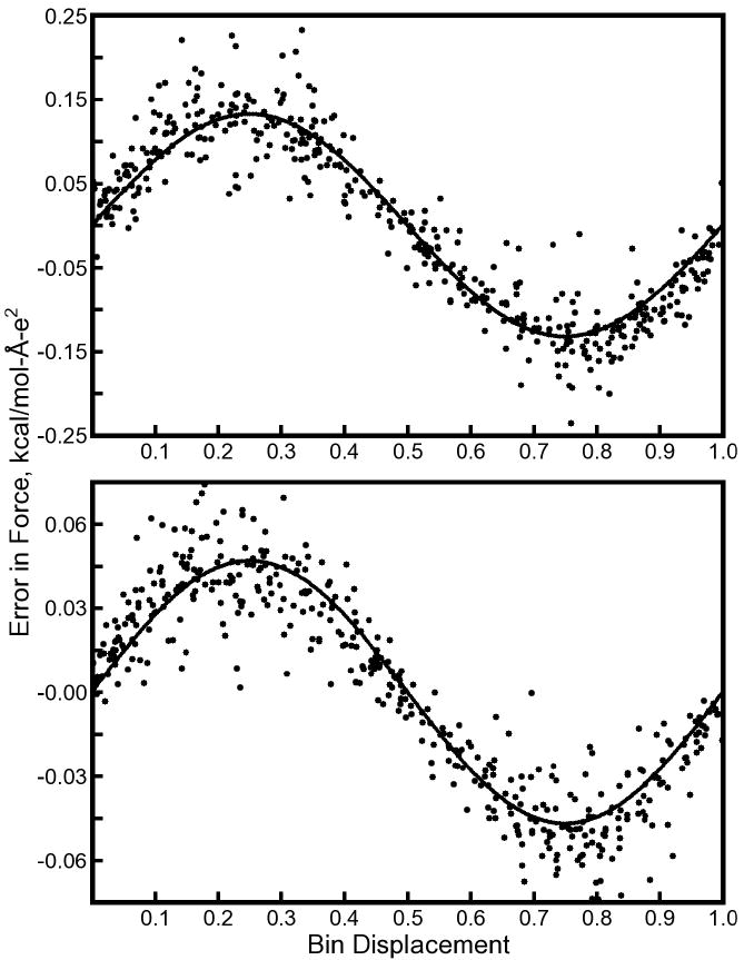
Figure 5. Force errors associated with pair interactions due to coarse reciprocal space meshes.

Significant errors enter the calculation of the force between two ±1e charges P₁ and P₂ when a coarse mesh (in this case, μ = 1.333Å) is used. Error in the x component of the force exerted on P₁ by P₂, excluding any self image force, is plotted as P₂ is moved parallel to the x axis such that its path intercepts P₁ unless otherwise noted. Results for several different positions of P₁ are shown as a function of the x displacement between P₁ and P₂. Panel A, solid line: P₁ is positioned at the origin. Panel A, dashed line: P₁ is positioned at 0.5μ along the x axis. In Panel B, the solid line is copied from Panel A but for the dashed line P₁ is positioned at (0.5μ, 0.5μ, 0.5μ). The errors are anticorrelated in Panel A and more strongly so in Panel B (the solid line with circles shows the average of the two errors). Panels C and D follow the format of Panel B. Panel C, solid line: P₁ positioned at 0.25μ on the x axis. Panel C, dashed line: P₁ positioned at (0.75μ, 0.5μ, 0.5μ). Panel D, solid line: P₁ positioned at (0.307μ, 1.421μ, 1.804μ), P₂ moved along the x axis. Panel D, dashed line: P₁ positioned at (0.807μ, 1.921μ, 2.804μ), P₂ moved to sample points (x, 0.5μ, 0.5μ).

As shown in Figure 5, different aliases of each particle interact in complex ways, giving rise to errors that depend both on the interparticle separation in all three dimensions as well as the bin displacement of the first charge. Despite these complexities, however, Figure 5 confirms that mesh staggering eliminates a majority of the pair interaction force errors, particularly if the two meshes are staggered by 1/2 the mesh spacing μ in all directions simultaneously. Chen and co-workers used this multi-dimensional staggering approach in their simulations of plasmas,¹⁶ although other investigators⁷ have suggested that the results of as many as eight meshes, staggered by μ/2 along any and all of the unit cell lattice vectors, should be averaged to obtain the best results. We tried averaging the results of eight such meshes (data not shown), but found this much more expensive approach to give scarcely better results than using only two meshes.

5.3 The Staggered Mesh Ewald method

Having confirmed that mesh staggering can eliminate large portions of the self interaction force error as well as pair interaction force errors in the SPME method, we sought to quantify the benefits of the mesh staggering in terms of accuracy and overall calculation efficiency when applied to condensed-phase biomolecular systems.

We term the use of two reciprocal space calculations on meshes aligned one half mesh spacing relative to one another in all three mesh dimensions “Staggered Mesh Ewald” (StME). Because the reciprocal space operations (mapping charges to the mesh, convoluting the density and solving Poisson’s equation, and interpolating forces from the smoothed potential) are identical to the procedures in SPME, implementing this method in current molecular dynamics codes can be straightforward. However, we will suggest some additional optimizations later in the Results.

With two meshes to compute but the potential to increase the accuracy by an order of magnitude or more relative to the corresponding SPME calculation, we wanted to thoroughly characterize the numerical error of StME relative to SPME for a variety of simulation parameters. In the 1970s, FFT solvers were efficient with mesh sizes of powers of 2—at the time, ”interlacing” typically meant using two coarse meshes with twice the spacing of the equivalent fine mesh, and delivered an intermediate level of accuracy. Modern FFT solvers, however, are able to work efficiently with multiples of 2, 3, 5, and even 7; we therefore have much more freedom in the choice of mesh spacings for maximizing efficiency. Furthermore, since the 1970s, simulations in non-orthorhombic unit cells have become more common; it is important to confirm that mesh staggering is beneficial in these cases as well.

We performed both SPME and StME calculations on all test cases listed in Table 1 and compared them to regular Ewald calculations as described in Methods. The results are plotted in Figures 6 and 7. These tests, which included non-cubic and non-orthorhombic cells, demonstrate the applicability of the method to periodic systems in general. Note, however, that the mesh grids are staggered by (1 /2)(v_a + v_b + v_c), not simply by the half the mesh spacing in x, y, and z.

Figure 6. Accuracy of Smooth Particle Mesh Ewald (SPME) and Staggered Mesh Ewald (StME) calculations for the streptavidin test case.

Each type of Ewald calculation was run using the parameters given in the top right corner of each panel. Black lines with open or filled symbols represent 4^th or 5^th order interpolation, respectively; diamonds and circles represent SPME and StME calculations, respectively. In most MD codes, a mesh of 90³ points would be used, along with D_tol = 1.0×10⁻⁵ or 1.0×10⁻⁶ and 4^th order interpolation; these cases are shown in orange and blue, respectively, for reference. Additional details of the streptavidin system are given in Table 1. Even with a mesh spacing 1.5× the standard value, the StME method offers improved accuracy over the corresponding SPME calculation for nearly all values of L_cut. StME maintains its advantage with finer meshes or higher interpolation orders.

Figure 7. Accuracy of SPME and StME calculations for three other test cases.

The format follows Figure 6 but only the case of a mesh spacing 1.5× the default value, that is μ approaching 1.5Å, is shown. The 35% v/v glycerol:water mixture, protein lattice, and the solvated COX-2 dimer are simulated in monoclinic, orthorhombic, and truncated octahedral cells, respectively. For efficiency, the truncated octahedron is tiled and reshaped into a triclinic unit cell in dynamics simulations. Additional details of all systems can be found in Table 1. The StME method shows comparable performance relative to SPME across all test cases.

Figures 6 and 7 show that, for a given order of interpolation and direct sum tolerance, the StME method can greatly increase the accuracy of computed forces relative to an SPME calculation with similar parameters. In all systems, error reductions exceeding one order of magnitude can be obtained for direct space cutoffs of 8Å to 10Å with similar mesh sizes and values of D_tol; the benefits of StME appear to be highest for direct space cutoffs and mesh densities near those used in typical MD simulations. Furthermore, the StME method continues to produce comparable increases in accuracy, relative to SPME, if the order of interpolation is increased or if D_tol is reduced. Although we did not demonstrate that the self image forces and errors in pair interaction forces could be cancelled with staggered meshes in non-orthorhombic unit cells, StME shows equally good performance for other condensed-phase systems in such unit cells.

While electrostatic potentials from two meshes must be computed in StME, the method achieves comparable accuracy to SPME with coarser meshes and smaller values of L_cut. For example, when using 4^th order interpolation and D_tol = 1.0×10⁻⁵ for calculations on the streptavidin system, StME achieves nearly the same accuracy with L_cut = 8.0Å and G_a = G_b = G_c = 60 as SPME with L_cut = 9.0Å and G_a = G_b = G_c = 90. In such a case, the direct space workload is reduced by almost 30% and the overall FFT workload is reduced by more than 40%: each mesh of 60³ points is 3.375× smaller than the mesh of 90³ points that would become the bottleneck for the SPME calculation. Twice as many charge mapping and force interpolations would be required in the most basic implementation of StME, but as will be discussed, other optimizations can still lead to significant improvements in simulation efficiency with this method. We will make a detailed analysis of the optimal parameters for StME and SPME calculations later in the results.

5.4 Energies and virials obtained with Staggered Mesh Ewald

Highly accurate forces are the most important product of a molecular dynamics method, but we also wanted to test whether StME could produce energies and virials of comparable accuracy to SPME, particularly when used with coarser meshes. Typically, electrostatics dominates the total potential energy of a molecular system but the energy of the reciprocal space part is fairly small. The reciprocal space calculation also makes fairly minor contributions to the system’s virial tensor. Still, errors in these contributions could limit the overall applicability of StME. We also tested whether errors in either of these quantities were systematic or random by repeating the StME and SPME calculations for 20 individual snapshots taken at 100ps intervals from 2ns trajectories of each system. These tests were conducted using the SANDER module of the AMBER software.

When the mesh used to compute the reciprocal space electrostatic potential is coarsened, both the energy and elements of the virial tensor trace become increased relative to their values obtained with a very fine mesh. Figure 8 shows that for a mesh spacing μ approaching 1.5Å, the reciprocal space calculation begins to report energies noticeably different from the values obtained in the limit of a very fine mesh. This behavior holds for the reciprocal space contributions to the virial trace as well; the off-diagonal elements of the virial accumulate very large errors (data not shown).

Figure 8. A removable bias in StME estimates of electrostatic energy and elements of the virial tensor trace.

In the left panel, StME using 60³ mesh points, 4^th order interpolation, D_tol = 1.0×10⁻⁵, and L_cut = 8.0Å estimates the streptavidin test system’s electrostatic energy 38.5 kcal/mol too high relative to a very accurate standard, on average, over the course of a 2ns simulation. The StME error in the energy estimate is given by the solid line with open circles; plain solid and dashed lines show the error if either of the two StME meshes were used alone. In comparison, a standard SPME calculation run with the AMBER default parameters (a mesh of 90³ points) delivers an error of only 0.6 ± 0.1 kcal/mol. However, the errors in the reciprocal space energy estimates of each StME mesh are strongly anticorrelated such that the overall error is very consistent: 38.5 ± 0.2 kcal/mol. If the 38.5 kcal/mol bias is removed by measuring against a high accuracy standard occasionally over the course of a simulation, the electrostatic energy can be consistently estimated to within the error of the AMBER default parameters. A similar treatment can be applied to derive the correct reciprocal space virial tensor trace, as shown for the COX-2 test case in the right panel (StME was performed with meshes of 80³ points; the default AMBER parameters imply a mesh of 120³ points for SPME). The format of the lines is the same; error in V_xx appears in the bottom half of plot, error in V_zz in the top half (error in V_yy is omitted for clarity).

Despite these limitations, it appears that StME can hold its ground in most constant pressure simulations and in cases when the total system energy is required. In any periodic simulation cell, isotropic position rescaling can be used to adjust the cell size to satisfy a particular external pressure making use of only the trace of the virial tensor. In orthorhombic cells, even anisotropic rescaling can be accomplished without reference to the virial’s off-diagonal elements. In our test cases, elements of the virial’s trace are consistently biased by nearly the same amount for a given system and a particular set of SPME parameters.

In StME calculations, the strong anti-correlation between the errors of the two coarse meshes carries over into estimates of the energy and virial trace, so that the average of the two results is biased more consistently than either alone. It is likely that the necessary correction factors can be computed at the beginning of a simulation by comparing the results from both StME meshes to the results from a finer mesh or higher interpolation order computed with the same values of D_tol and L_cut. Periodic updates of the correction factors, perhaps every 10,000 steps or upon significant changes in the unit cell dimensions, appear to be a reliable means of keeping errors in the calculated energy and virial trace within the levels obtained with conventional SPME calculations and accepted parameters. To ensure that the accuracy in estimates of the energy and virial trace (after removing the bias) was comparable to the accuracy of forces in StME, we scanned over a large number of all four Ewald parameters for the streptavidin and COX-2 test cases. The results in Figure 9 confirm that, if StME produces accurate forces, it produces a precise virial trace and energy as well. Further explanation of why the energy and virial trace estimates are biased in the manner observed is provided in the Supporting Information.

Figure 9. Error in energy and virial trace elements plotted against error in forces obtained by the StME method.

Forces, energies, and virials were computed by StME for 20 snapshots of the streptavidin and COX-2 test cases for D_tol of 1.0×10⁻⁵ or 1.0×10⁻⁶, μ ranging from 2.0 to 0.9Å, L_cut ranging from 7 to 12Å, and 4^th or 5^th order interpolation. Each point in the four plots above represents the results for a particular set of Ewald parameters: the root mean squared error in electrostatic energy or instantaneous pressure (after removal of any bias) is plotted against the average force rmsd for all 20 snapshots. The division of the points into two groups stems from the different values of D_tol. Crosshairs in each plot intersect at the error in force and error in pressure or energy obtained using the default AMBER parameters (μ ≤1Å, 4^th order interpolation, L_cut = 8.0Å, and D_tol = 1.0×10⁻⁵) for each system. Although the errors in pressure may appear large, only the amplitude is plotted and after removal of bias the error in pressure from StME calculations can be positive or negative. The root mean squared deviations in the instantaneous pressure obtained for streptavidin and COX-2 over the course of each simulation were both 90 bar, fluctuating about an average of 1 bar; in this sense, the errors in pressure are a miniscule amount of extra noise.

5.5 A simple metric for the accuracy of Ewald mesh methods

As in shown in the Supporting Information, it is logical to compute the accuracy of the reciprocal space part of an Ewald mesh calculation as a function of σ/μ, where σ is the width of the Gaussian charge smoothing function defined in Equation S.1 of the Supporting Information and μ, again, is the mesh spacing. We did this for all four of our test cases by computing SPME or StME calculations for σ ranging from 0.5 to 3.0Å, μ ranging from 0.9 to 2.0Å, and 4^th, 5^th, or 6^th order interpolation.

Force errors for each test case are plotted as a function of σ/μ in Figure 10 for StME calculations using 4^th order interpolation and SPME calculations using 4^th, 5^th, or 6^th order interpolation. In all cases, the accuracy of forces appears to approach a log-linear relationship with σ/μ; in this region, the accuracy of StME is roughly 1.2 orders of magnitude higher than SPME with identical parameters.

Figure 10. Accuracy of forces as a function of the ratio of charge smoothing to mesh spacing.

In each of four systems, the accuracy of forces was computed for a range of values of direct space cutoff L_cut and mesh spacing μ. For all calculations, the direct sum tolerance D_tol was set to 1.0×10⁻⁹, implying that errors in the forces came almost exclusively from the reciprocal space calculation. Equation S.7 of the Supporting Information was used to obtain the width of the Gaussian charge smoothing function in each calculation. Each plot is marked according to the “AMBER” and “CHARMM” accuracy standards, assuming that the reciprocal space calculation must create errors not in excess of half the level of each standard. The accuracy of the reciprocal space calculations as a function of σ/μ is a logical way to compare StME and SPME with different orders of interpolation: it indicates how aggressively the charges must be smoothed and hence provides an indication of how long L_cut must be for a particular μ. By this metric, StME with 4^th order interpolation performs slightly better than SPME with 6^th order interpolation to obtain the levels of accuracy sought in most molecular simulations.

Because the accuracy in an Ewald mesh calculation also depends on contributions from the direct space calculation, we assumed that the entire electrostatics calculation could meet “AMBER” or “CHARMM” accuracy if the reciprocal space calculation produced errors up to half the level of either standard (this estimate is conservative, as the direct and reciprocal space forces for any given atom are generally oriented randomly with respect to one another, so the magnitude of the combined error will be at most the sum of the direct and reciprocal space errors). Our findings echo results in Figures 6 and 7: StME calculations using 4^th order interpolation can meet the “AMBER” level of accuracy with σ ≥ 1.0μ, whereas SPME run with 4^th order interpolation would require σ ≥ 1.5μ. This is reflected in the AMBER default parameters: L_cut = 8.0Å and D_tol = 1.0×10⁻⁵ implies that σ is approximately 1.42Å to pair with μ ≤ 1Å. Similarly, StME can achieve “CHARMM” accuracy using 4^th order interpolation and σ ≥ 1.2μ. SPME with 4^th order interpolation would require σ ≥ 2.0μ: this is reflected by the NAMD recommended parameters L_cut = 12.0Å and D_tol = 1.0×10⁻⁶, implying σ ~ 1.94 Å for μ ≤ 1Å. Figure 10 also shows that SPME calculations must use 6^th order interpolation to produce “AMBER” or “CHARMM” accuracy with the σ/μ ratios available to StME with 4^th order interpolation.

In the Supporting Information, we show that there is a nearly linear relationship between σ and L_cut for a given D_tol, which implies that there is then a roughly linear relationship between the acceptable values of L_cut and μ for a given value of D_tol. In the next section, we will examine how the combination of μ, L_cut, and D_tol can be used to optimize performance in both SPME and StME.

5.6 Optimal StME and SPME parameters

In order to define optimal Ewald parameters, we return to the “AMBER” and “CHARMM” accuracy standards as defined in Methods. Because different computing architectures favor different levels of real-space or reciprocal space calculations, we did intensive scans of L_cut between 6.0 and 16.0Å, μ between 0.7 and 2.0Å and D_tol between 5.0×10⁻⁷ and 1.0×10⁻⁵ for both 4^th and 5^th order interpolation. Because the choice of D_tol does not affect execution time, we sought any value of D_tol that could satisfy the accuracy standards for given values of L_cut and μ. Results for SPME and StME methods are plotted in Figure 11.

Figure 11. Ewald parameters yielding “AMBER” or “CHARMM” levels of accuracy in the streptavidin and COX-2 test cases.

By scanning L_cut and μ for different orders of interpolation and optimizing D_tol for greatest accuracy in each case, we were able to determine the region of the L_cut and μ parameter space on which SPME or StME give acceptable levels of accuracy. The format of boundary lines in each panel follows Figure 6: diamonds denote the SPME method and circles denote the StME method, while open and filled symbols denote 4^th and 5^th order interpolation, respectively. Values of L_cut and μ below and to the right of each boundary line produce accurate forces according to the standard listed in each panel.

While increasing the interpolation order from 4 to 5 will greatly expand the combinations of L_cut and μ that can produce a particular level of accuracy, staggered meshes with 4^th order interpolation offer an even wider array of options. Figure 11 also confirms a result evident in Figures 6 and 7, that increasing the interpolation order with staggered meshes is of marginal benefit when seeking the “AMBER” level of accuracy, but offers more significant improvements when seeking the higher “CHARMM” level of accuracy.

Although we do not have a working version of Staggered Mesh Ewald in an efficient molecular dynamics package, it is not difficult to obtain reasonable estimates of the single-processor efficiency of StME versus SPME. We assume that the costs of the occasional energy and virial bias corrections and the cost of averaging the forces obtained by the two reciprocal space calculations are negligible. If the two reciprocal space calculations share data, the computation of the reciprocal space pair potential θ̂^(rec) need only be done once for both meshes, and there is even the possibility of using “harmonic averaging,”¹⁷ combining the two staggered meshes in Fourier space to eliminate one of the four FFTs and one of the two force interpolation procedures for significant overall savings. However, we assumed that the two calculations must be done independently, because there may be benefits to parallel performance in this regard and independent calculations make the StME implementation trivial. Under these assumptions, the reciprocal space part of an StME calculation takes exactly twice as long as the identical SPME reciprocal space calculation. Tests were conducted on an Intel 2.66GHz E5430 processor with the serial version of the pmemd module of AMBER10. Similar to findings presented by Crocker and co-workers in the development of their own parameter optimization program MDSimAid,²³ we were unable to significantly improve the performance of single-processor SPME calculations by simply adjusting the parameters. However, Tables 2 and 3, which also provide additional details of the molecular dynamics benchmark, shows that optimized StME parameters can perform somewhat better than optimized SPME parameters to obtain either “AMBER” or “CHARMM” accuracy on the four test cases.

Table 2.

Timings for optimal Smooth Particle Mesh Ewald (SPME) parameters and estimated timings for Staggered Mesh Ewald (StME) parameters. Each system, described in Table 1, was run for 1000 steps in the NVT ensemble using a 1fs time step, Berendsen thermostat, 10Å cutoff on Lennard-Jones interactions, 2Å nonbonded pairlist buffer, and the stated electrostatic parameters. The internal geometry of water molecules was constrained by SETTLE;³⁶ the lengths of other bonds to hydrogen were constrained by SHAKE.³⁷ Reciprocal space electrostatics were computed at every time step using the stated parameters and 4^th order interpolation. Timings for StME were estimated by doubling the reciprocal space calculation time of an SPME calculation run with the same parameters. This test used 4^th order interpolation exclusively because higher orders are very rarely used in practice and many codes, including the PMEMD version used for this test, use optimized routines for 4^th order interpolation. While we were able to obtain better overall run times by using higher orders of interpolation in the SPME runs, it would also be possible to improve the efficiency of StME runs if the two reciprocal space calculations were able to share data. This test is meant to offer a basic estimate of the efficiency of StME.

	Run Parameters			Timings
Method	Lcut, Å	Dtol	Mesh Size	Dir.b	Rec.c	Totald	Factore
Streptavidin, AMBER Accuracy
SPME	8.5	4.0×10−6	96 × 96 × 96	362	123	584	1.00
StME	6.5	4.0×10−6	80 × 80 × 80	244	156	498	1.17
Streptavidin, CHARMM Accuracy
SPME	10.0	5.0×10−7	120 × 120 × 120	482	218	792	1.00
StME	8.5	8.0×10−7	80 × 80 × 80	360	156	615	1.29

^aOrder of interpolation

^bDirect space interaction computation time, including van der Waals interactions (all timings are in seconds)

^cReciprocal space computation time

^dTotal simulation time, including nonbonded pairlist updates and bonded atom force calculations

^eOverall rate of simulation, relative to SPME

Table 3.

Timings for optimal Smooth Particle Mesh Ewald (SPME) parameters and estimated timings for Staggered Mesh Ewald (StME) parameters. The format, molecular dynamics benchmark protocol, and labeling follows Table 2. StME performs better than SPME across all systems studied, though parallel scaling for an optimized StME implementation has not yet been tested.

	Run Parameters			Timings
Method	Lcut, Å	Dtol	Mesh Size	Dir.b	Rec.c	Totald	Factore
Glycerol, AMBER Accuracy
SPME	8.5	5.0×10−6	72 × 72 × 90	219	86	369	1.00
StME	8.0	7.0×10−6	48 × 48 × 60	200	68	332	1.11
Glycerol, CHARMM Accuracy
SPME	10.0	5.0×10−7	96 × 96 × 120	284	190	534	1.00
StME	8.5	9.0×10−7	64 × 64 × 80	222	119	405	1.32
Crystal, AMBER Accuracy
SPME	8.0	7.0×10−6	90 × 96 × 96	487	117	747	1.00
StME	7.5	8.0×10−6	64 × 60 × 64	462	100	700	1.07
Crystal, CHARMM Accuracy
SPME	10.0	1.0×10−6	120 × 108 × 120	588	200	926	1.00
StME	9.0	1.0×10−6	72 × 64 × 72	540	117	795	1.16
Cyclooxygenase-2, AMBER Accuracy
SPME	8.5	5.0×10−6	120 × 120 × 120	614	330	1127	1.00
StME	7.0	5.0×10−6	100 × 100 × 100	458	417	1056	1.07
Cyclooxygenase-2, CHARMM Accuracy
SPME	10.0	8.0×10−7	160 × 160 × 160	782	719	1696	1.00
StME	9.0	8.0×10−7	100 × 100 × 100	675	421	1281	1.32

In contrast to single-processor performance, parallel scaling is difficult to predict. We expect that the performance advantage of StME will carry over into simulations on small numbers of processors and that the ability to reduce the overall FFT workload without increasing the direct space workload will give StME another advantage in highly parallel applications. The optimal parameters will change with the number of processors, and as shown in Figure 11 StME offers many choices. Parallel implementations of the SPME algorithm have been extensively optimized for parallel scaling by multiple independent groups;^13,14,15 while StME can likely benefit from much of this progress, it will take some effort to devise a parallel StME implementation that is as finely tuned in order to make a fair comparison with the best SPME implementations.

6 Discussion

In this communication, we have reviewed and renewed an old technique, “interlacing,” for improving the accuracy of particle:mesh calculations. While the technique was originally used to reduce the memory requirements of such calculations at the expense of simulation speed, our new implementation “Staggered Mesh Ewald” seems to confer some benefits to overall speed on modern computers. Nowadays, computer memory is plentiful but the ability to use smaller meshes may help to reduce the total communication cost of simulations in parallel applications. We will now discuss how mesh staggering might benefit other Ewald mesh methods, Poisson solvers, and molecular simulations.

6.1 Staggered meshes for other Poisson solvers

Previously, mesh staggering has been shown to be effective with the Particle:Particle Particle:Mesh (P³M) method,¹⁷ and here we have shown it to be effective with the Smooth Particle Mesh Ewald (SPME) method. The principal difference between these electrostatic methods is the shape of the charge smoothing function used in the mesh calculation: P³M uses a spherical hypercone, whereas SPME uses a spherical Gaussian, which confers some advantage in accuracy⁹ because the Gaussians are better at conserving the total amount of charge on the mesh. We expect that mesh staggering will also improve the accuracy of Gaussian Split Ewald (GSE) calculations,⁹ which are nearly identical to SPME except in the function used to interpolate particles to the mesh (SPME uses a B-spline whereas GSE uses another Gaussian, but B-splines in fact converge to Gaussians in the limit of high interpolation order²⁴).

Another possible application of mesh staggering is to real-space variants on the SPME method, which use the same particle interpolation and charge smoothing functions but solve Poisson’s equation in real space^10,11. These methods may prove more scalable than FFT-based methods on very high numbers of processors, but the principal drawback of these methods is the cost of smoothing the charge density in real space, a function of the number of mesh points. Staggered meshes can not only reduce the number of mesh points needed, they can also improve the efficiency of the charge smoothing procedure because the distances between corresponding mesh points are identical on both meshes. Such improvements may help close the gap between real-space and FFT-based Poisson solvers in Ewald calculations.

Fast Multipole methods (FMMs)^25,26 receive attention for the same reasons as real-space based Poisson solvers: the promise of O(N) scaling and also exponentially reduced communication requirements as the interactions become increasingly long-ranged. While FMMs continue to be slower than FFT-based Poisson solvers for condensed phase molecular systems, as with real-space Poisson solvers, considerable progress has been made in recent years. It is possible that staggering the hierarchy of meshes used by FMMs may confer the same benefits as staggering the one mesh used by SPME or P³M, again helping to close the performance gap between these methods and the standard particle:mesh techniques used in most molecular simulations.

While mesh staggering may have utility in other Poisson solvers, other approximations that have proven useful in standard Poisson solvers may be of utility in Staggered Mesh Ewald. In particular, the use of spherically truncated FFTs,²⁷ discarding very low-frequency modes in Fourier space much as interactions in the tail of the direct space sum are discarded in standard SPME, can decrease the cost and communication requirements of the FFT needed to take the charge Q mesh into Fourier space. By using spherically truncated FFTs and harmonic averaging¹⁷ in the context of Staggered Mesh Ewald, the communication requirements and cost of evaluating the FFTs for the reciprocal space sum might be reduced even further.

6.2 Staggered Mesh Ewald for highly parallel applications

We have not presented results for the performance of StME in the context of parallel molecular dynamics simulations because we do not yet have a working implementation in this respect. We have shown that StME offers moderate performance improvements on single-processor simulations, which can be expected to carry over into parallel applications on small numbers of processors. The scaling of highly parallel algorithms is difficult to predict, but we will address three of the most critical aspects of the reciprocal space calculation with respect to parallel implementations and StME.

On large numbers of processors, the scaling of the Ewald reciprocal space calculation is limited primarily by the number of messages that must be passed between processors in order to accomplish the FFT operations for convoluting the charge mesh Q with the reciprocal space pair potential θ^(rec). If P nodes are working together to compute an FFT, each node must send its part of the FFT data to all other nodes, and receive FFT data from all other nodes. (It is for this reason that most codes devote a subset of processors to the reciprocal space calculation.) Because StME requires up to 40% less FFT work than regular SPME, the FFTs could be performed on a smaller subset of processors, implying fewer messages to pass.

But, reducing the amount of mesh data can imply other communication costs. A second important factor in the cost of a parallel reciprocal space calculation is the cost of communicating the coordinates and identities of atoms in order to construct the charge mesh Q, before any FFTs take place at all. In SPME with n^th order interpolation, each atom influences a rectangular region of the mesh Q that is nμ points on each side. As n or μ increases, more atoms must be therefore imported from further away in order to consruct Q. As was shown in the results, StME with 4^th order interpolation produces similar accuracy to SPME with 6^th order interpolation, all other parameters being equal. StME could therefore make use of a large μ such as 1.5Å with smaller import regions for constructing Q than SPME would require. However, the import regions would still be somewhat larger than those required by an SPME calculation using the typical μ = 1Å.

A third factor that influences the cost of a parallel reciprocal space calculation is the actual cost of constructing Q and then interpolating forces from the potential Q ⋆ θ^(rec). These particle ↔ mesh operations, which can be more expensive than the FFTs themselves (data not shown), are typically performed on the same processors that will do the convolution Q ⋆ θ^(rec). Because StME essentially doubles the cost of the particle ↔ mesh operations, it may be difficult to reduce the number of processors devoted to the FFT operations. However, the particle ↔ mesh operations can be done on the more numerous processors devoted to the direct space calculation so that the grid data itself could be communicated to a subset of processors for computing the convolution. NAMD¹⁵ is already equipped to run traditional SPME calculations by passing mesh data, not coordinates, to reciprocal space processors when the highest possible scaling is desired; such a reorganization may be necessary in order to make StME beneficial to highly parallel applications.

6.3 Continued improvement of Ewald mesh methods

Ewald mesh methods will likely remain an important tool for molecular simulations well into the future. Briefly, calculating long-ranged Coulomb electrostatics currently accounts for a majority of the total simulation time, and will continue to do so even as classical models begin to incorporate other charge geometries and explicit polarization effects. While quantum effects are undoubtedly important for the interaction of charges at very short range, the Coulomb approximation quickly takes over even on molecular scales. Furthermore, numerous studies have shown that the periodic boundary conditions enforced by Ewald mesh methods are relatively benign, especially in comparison to some alternatives. We will describe the rationale for continued development of Ewald electrostatics in more detail, then outline other avenues to accelerating Ewald calculations which we hope will dramatically accelerate traditional Ewald mesh calculations and serve as a powerful complement to the Staggered Mesh Ewald method.

The majority of the computational effort in molecular dynamics simulations is devoted to electrostatic nonbonded interactions, whereas the calculation of van der Waals dispersion interactions, typically by Lennard Jones potentials, is minor in comparison. Primarily, this is because electrostatic interactions are very long ranged. Moreover, because of the form of the electrostatic potential, analytic electrostatic force computations require not only a divide operation but also an expensive square root operation to obtain the quantity $\left[k_{\mathrm{coul}}{q}_i{q}_j/r_{\mathit{ij}}^3\right]{\mathbf{r}}_{\mathit{ij}}$ where k_coul is Coulomb’s constant, q_i and q_j represent charges of the atoms i and j, and r_ij is the vector between the charges. In contrast, the Lennard-Jones force requires only a divide operation to compute the quantity $\left[A_{\mathit{ij}}/r_{\mathit{ij}}^8+B_{\mathit{ij}}/r_{\mathit{ij}}^{14}\right]{\mathbf{r}}_{\mathit{ij}}$, where A_ij and B_ij are constants. A third factor that makes electrostatic calculations dominate the cost of simulations is a peculiarity of current water models, most of which give Lennard Jones attributes to only the oxygen atoms while placing charges on at least three sites. Because water makes up the majority of the system in most simulations of solvated proteins, there can be many more electrostatic interactions than Lennard-Jones interactions for a given cutoff.

While point charges may not be an adequate representation of atomic charge distributions at close range,²⁸ Ewald mesh methods are also compatible with other charge geometries. One must merely recall that the direct space interactions are a modification to the electrostatic potential of the smoothed charge distribution computed in the reciprocal space calculation, as discussed in the Introduction and Methods. The direct space modification can just as easily be used to extract interactions of distributed charges, so long as the interaction of two charges in the actual system and the interaction of two Gaussian charges converge at the direct space cutoff. Even if it does not perfectly describe the interaction of subatomic particles at close range, Coulomb’s law is still valid for the interaction of charges on the nanometer scale. Therefore, long-ranged electrostatic methods such as the Ewald sum will continue to be essential for molecular simulations, even as new force fields with different local electrostatic approximations and even explicit polarization effects²⁹ come into use.

There is debate over whether periodicity imposed by Ewald electrostatics is suitable for molecular simulationss,^30,31 and while such a representation may be much more appropriate for crystal lattice simulations,³² periodic boundary conditions are a very practical solution for simulations of proteins in boxes of water as well. While there are relevant concerns when using periodic boundary conditions with very small systems,³³ finite size effects are by no means limited to periodic systems. Simulations performed in both periodic and non-periodic unit cells such as droplets³⁴ or ice shells³⁵ suggest that periodic boundary conditions are as good or better than numerous alternatives.

Given the importance of Ewald mesh methods to molecular simulations, further developments that permit the use of coarser meshes or reduce the required number of direct space computations are of great interest. In this communication, we have analyzed the errors arising from a coarse mesh in terms of self image forces and pair interaction force errors. The self image forces we identified can be corrected on a per-atom basis for low-density plasma simulations, but the pair interaction force errors arising from a coarse mesh require more extensive corrections in condensed-phase simulations. Our solution was to introduce a second mesh calculation, staggered relative to the original. It may also be possible to modify the form of the Ewald “switching” function used to make the transition between the reciprocal space electrostatic potential and the direct space modification. The form used in all Ewald mesh methods to date, most apparent in Equation 1, is dictated by the form of the charge smoothing function, a Gaussian as described in Equation S1. of the Supporting Information. The typical direct space potential satisfies the most important property of an Ewald switching function in that it smoothly vanishes within a reasonable distance, while the associated Gaussian function ensures that charges can be mapped to a mesh with reasonable accuracy. However, it may be possible to design new charge smoothing and potential switching functions that map charges more accurately to coarser meshes or vanish more rapidly. We are pursuing new ways to satisfy these criteria and expect the results to be generally useful for all types of Ewald mesh calculations.

References

- 1.Beck DAC, Daggett V. Methods for molecular dynamics simulations of protein folding/unfolding in solution. Methods. 2004;34:112–120. doi: 10.1016/j.ymeth.2004.03.008. [DOI] [PubMed] [Google Scholar]
- 2.Hess B, Kutzner C, van der Spoel D, Lindahl E. GROMACS 4: Algorithms for highly efficient, load-balanced, and scalable molecular simulation. J Chem Theory Comput. 2008;4:435–447. doi: 10.1021/ct700301q. [DOI] [PubMed] [Google Scholar]
- 3.DeLeeuw SW, Perram JW, Smith ER. Simulation of Electrostatic Systems in Periodic Boundary Conditions. I. Lattice Sums and Dielectric Constants. Proc R Soc Lond Ser A. 1980;373:27–56. [Google Scholar]
- 4.Yonetani Y. A severe artifact in simulation of liquid water using a long cut-off length: Appearance of a strange layer structure. Chem Phys Lett. 2005;406:49–53. [Google Scholar]
- 5.Patra M, Karttunen M, Hyvönen MT, Falck E, Lindqvist P, Vattulainen I. Molecular dynamics simulations of lipid bilayers: Major artifacts due to truncating electrostatic interactions. Biophys J. 2003;84:3636–3645. doi: 10.1016/S0006-3495(03)75094-2. [DOI] [PMC free article] [PubMed] [Google Scholar]
- 6.Pollock EL, Glosli J. Comments on P3M, FMM, and the Ewald method for large periodic Coulombic systems. Comput Phys Commun. 1996;95:93–110. [Google Scholar]
- 7.Hockney RW, Eastwood J. Computer Simulation Using Particles. Taylor and Francis Group; New York, New York: 1988. Collisionless Particle Models; pp. 260–291. [Google Scholar]
- 8.Essmann U, Perera L, Berkowitz ML, Darden T, Lee H, Pedersen LH. A smooth particle mesh Ewald method. J Chem Phys. 1995;103:8577–8593. [Google Scholar]
- 9.Shan Y, Klepeis JL, Eastwood MP, Dror RO, Shaw DE. Gaussian Split Ewald: A fast Ewald mesh method for molecular simulation. J Chem Phys. 2005;122:054101. doi: 10.1063/1.1839571. [DOI] [PubMed] [Google Scholar]
- 10.Sagui C, Darden T. Multigrid methods for classical molecular dynamics simulations of biomolecules. J Chem Phys. 2001;114:6578–6591. [Google Scholar]
- 11.Beckers JVL, Lowe CP, De Leeuw SW. An iterative PPPM method for simulating coulombic systems on distributed memory parallel computers. Mol Simulat. 1998;20:369–383. [Google Scholar]
- 12.Darden T, York D, Pedersen L. Particle mesh Ewald: An N · log(N) method for Ewald sums in large systems. J Chem Phys. 1993;98:10089–10092. [Google Scholar]
- 13.Case DA, Darden TA, Cheatham TE, III, Simmerling CL, Wang J, Duke RE, Luo R, Crowley M, Walker RC, Zhang W, Merz KM, Wang B, Hayik S, Roitberg A, Seabra G, Kolossváry I, Wong KF, Paesani F, Vanicek J, Wu X, Brozell SR, Steinbrecher T, Gohlke H, Yang L, Tan C, Mongan J, Hornak V, Cui G, Mathews DH, Seetin MG, Sagui C, Babin V, Kollman PA. AMBER 10. University of California; San Francisco: San Francisco, CA, USA: 2008. [Google Scholar]
- 14.Bowers KJ, Chow E, Xu H, Dror RO, Eastwood MP, Gregersen BA, Klepeis JL, Kolossváary I, Moraes MA, Sacerdoti FD, Salmon JK, Shan Y, Shaw DE. Scalable algorithms for molecular dynamics simulations on commodity clusters. Conference on High Performance Networking and Computing, Proceedings of the 2006 ACM/IEEE conference on Supercomputing; Tampa, FL, USA. 2006; New York, NY: Association for Computing Machinery; 2006. [Google Scholar]
- 15.Phillips JC, Braun R, Wang W, Gumbart J, Tajkhorshid E, Villa E, Chipot C, Skeel RD, Kale L, Sand chulten K. Scalable molecular dynamics with NAMD. J Comput Chem. 2005;26:1781–1802. doi: 10.1002/jcc.20289. [DOI] [PMC free article] [PubMed] [Google Scholar]
- 16.Chen L, Langdon B, Birdsall CK. Reduction of the grid effects in simulation plasmas. J Comput Phys. 1974;14:200–222. [Google Scholar]
- 17.Eastwood J. Optimal P3M Algorithms for Molecular Dynamics Simulations. In: Hooper MB, editor. Computational Methods in Classical and Quantum Physics. Advance Publications Ltd; London, UK: 1976. pp. 206–228. [Google Scholar]
- 18.Hyre DE, Le Trong I, Merritt EA, Green NM, Stenkamp RE, Stayton PS. Wildtype core-streptavidin with biotin at 1.4Å. Protein Sci. 2006;15:459–467. doi: 10.1110/ps.051970306. [DOI] [PMC free article] [PubMed] [Google Scholar]
- 19.Smith GD, Blessing RH, Ealick SE, Fontecilla-Camps JC, Hauptman HA, Housset D, Langs DA, Miller R. Ab initio structure determination and refinement of a scorpion protein toxin. Acta Crystallogr D. 1997;53:551–557. doi: 10.1107/S0907444997005386. [DOI] [PubMed] [Google Scholar]
- 20.Kiefer JR, Pawlitz JL, Moreland KT, Stegeman RA, Gierse JK, Stevens AM, Good-win DC, Rowlinson SW, Marnett LJ, Stallings WC, Kurumbail RG. Structural insights into the stereochemistry of the cyclooxygenase reaction. Nature. 2000;405:97–101. doi: 10.1038/35011103. [DOI] [PubMed] [Google Scholar]
- 21.Chelli R, Procacci P, Cardini G, Cella Valle RG, Califano S. Glycerol condensed phases Part I. A molecular dynamics study. Phys Chem Chem Phys. 1999;1:871–877. [Google Scholar]
- 22.Hornak V, Abel R, Okur A, Strockbine B, Roitberg A, Simmerling C. Comparison of multiple Amber force fields and development of improved protein backbone parameters. Proteins. 2006;65:712–725. doi: 10.1002/prot.21123. [DOI] [PMC free article] [PubMed] [Google Scholar]
- 23.Crocker MS, Hampton SS, Matthey T, Izaguirre JA. MDSIMAID : Automatic parameter optimization in fast electrostatic algorithms. J Comput Chem. 2005;26:1021–1031. doi: 10.1002/jcc.20240. [DOI] [PubMed] [Google Scholar]
- 24.Unser M, Aldourbi A, Eden M. On the asymptotic convergence of B-spline wavelets to Gabor functions. IEEE Trans Inform Theo. 1992;38:864–872. [Google Scholar]
- 25.Lu B, Cheng X, McCammon JA. “New-version-fast-multipole-method” accelerated electrostatic calculations in biomolecular systems. J Comput Phys. 2007;226:1348–1366. doi: 10.1016/j.jcp.2007.05.026. [DOI] [PMC free article] [PubMed] [Google Scholar]
- 26.Lu B, Cheng X, Huang J, McCammon JA. Order N algorithm for computation of electrostatic interactions in biomolecular systems. Proc Natl Acad Sci U S A. 2006;103:19314–19319. doi: 10.1073/pnas.0605166103. [DOI] [PMC free article] [PubMed] [Google Scholar]
- 27.Fang B, Martyna G, Deng Y. A fine grained parallel smooth particle mesh Ewald algorithm for biophysical simulation studies: Application to the 6D-torus QCDOC supercomputer. Comput Phys Commun. 2007;177:362–377. [Google Scholar]
- 28.Paricaud P, Predota M, Chialvo AA, Cummings PT. From dimer to condensed phases at extreme conditions: Accurate predictions of the properties of water by a Gaussian charge polarizable model. J Chem Phys. 2005;122:244511. doi: 10.1063/1.1940033. [DOI] [PubMed] [Google Scholar]
- 29.Warshel A, Kato M, Pisliakov AV. Polarizable force fields: History, test cases, and prospects. J Chem Theory Comput. 2007;3:2034–2045. doi: 10.1021/ct700127w. [DOI] [PubMed] [Google Scholar]
- 30.Villareal MA, Montich GG. On the Ewald artifacts in computer simulations. The test-case of the octaalanine peptide with charged termini. J Biomol Struct Dyn. 2005;23:135–142. doi: 10.1080/07391102.2005.10507054. [DOI] [PubMed] [Google Scholar]
- 31.Hünenberger PH, McCammon JA. Ewald artifacts in computer simulations of ionic solvation and ion-ion interaction: A continuum electrostatics study. J Chem Phys. 1999;110:1856–1872. [Google Scholar]
- 32.Cerutti DS, Le Trong I, Stenkamp RE, Lybrand TP. Simulations of a protein crystal: Explicit treatment of crystallization conditions links theory and experiment in the streptavidin-biotin complex. Biochemistry. 2008;47:12065–12077. doi: 10.1021/bi800894u. [DOI] [PMC free article] [PubMed] [Google Scholar]
- 33.Weerasinghe S, Smith PE. A Kirkwood-Buff derived force field for mixtures of urea and water. J Phys Chem B. 2003;107:3891–3898. [Google Scholar]
- 34.Freitag S, Chu V, Penzotti JE, Klumb LA, To R, Hyre D, Le Trong I, Lybrand TP, Stenkamp RE, Stayton PS. A structural snapshot of an intermediate on the streptavidin-biotin dissociation pathway. P Natl Acad Sci USA. 1999;96:8384–8389. doi: 10.1073/pnas.96.15.8384. [DOI] [PMC free article] [PubMed] [Google Scholar]
- 35.Riihimäki ES, Martínez JM, Kloo L. An evaluation of non-periodic boundary condition models in molecular dynamics simulations using prion octapeptides as probes. J Mol Struc-Theochem. 2005;760:91–98. [Google Scholar]
- 36.Miyamoto S, Kollman PA. SETTLE: An analytical version of the SHAKE and RATTLE algorithm for rigid water models. J Comput Chem. 1992;13:952–962. [Google Scholar]
- 37.Ryckaert JP, Ciccotti G, Berendsen HJC, Hirasawa K. Numerical integration of the cartesian equations of motion of a system with constraints: Molecular dynamics of n-alkanes. J Comput Phys. 1997;23:327–341. [Google Scholar]
Associated Data
This section collects any data citations, data availability statements, or supplementary materials included in this article.