Predictive models of autism spectrum disorder based on brain regional cortical thickness

Abstract

Autism spectrum disorder (ASD) is a neurodevelopmental disorder with a wide phenotypic range, often affecting personality and communication. Previous voxel-based morphometry (VBM) studies of ASD have identified both gray- and white-matter volume changes. However, the cerebral cortex is a 2-D sheet with a highly folded and curved geometry, which VBM cannot directly measure. Surface-based morphometry (SBM) has the advantage of being able to measure cortical surface features, such as thickness. The goals of this study were twofold: to construct diagnostic models for ASD, based on regional thickness measurements extracted from SBM; and to compare these models to diagnostic models based on volumetric morphometry. Our study included 22 subjects with ASD (mean age 9.2 ± 2.1 years) and 16 volunteer controls (mean age 10.0 ± 1.9 years). Using SBM, we obtained regional cortical thicknesses for 66 brain structures for each subject. In addition, we obtained volumes for the same 66 structures for these subjects. To generate diagnostic models, we employed four machine-learning techniques: support vector machines (SVMs), multilayer perceptrons (MLPs), functional trees (FTs), and logistic model trees (LMTs). We found that thickness-based diagnostic models were superior to those based on regional volumes. For thickness-based classification, LMT achieved the best classification performance, with accuracy = 87%, area under the receiver operating characteristic (ROC) curve (AUC) = 0.93, sensitivity = 95%, and specificity = 75%. For volume-based classification, LMT achieved the highest accuracy, with accuracy = 74%, AUC = 0.77, sensitivity = 77%, and specificity = 69%. The thickness-based diagnostic model generated by LMT included 7 structures. Relative to controls, children with ASD had decreased cortical thickness in the left and right pars triangularis, left medial orbitofrontal gyrus, left parahippocampal gyrus, and left frontal pole, and increased cortical thickness in the left caudal anterior cingulate and left precuneus. Overall, thickness-based classification outperformed volume-based classification across a variety of classification methods.

1. Introduction

Autism spectrum disorder (ASD) is a neurodevelopmental disorder with a prevalence of approximately in 1 in 150 children (Amaral, et al. 2008). Children with ASD have abnormal social behavior, impaired communication and language skills, and repetitive/stereotyped behavior (Belmonte, et al. 2004; Nordahl, et al. 2007; Rapin 1997). In studies of cognition, ASD has been defined as fundamental deficits in central coherence, executive function, and empathizing (Belmonte, et al. 2004). MR examination has revealed that children with ASD have subtle structural changes in many brain structures, including the frontal lobe, parietal lobe, hippocampus, amygdala, cerebellum and brain stem (Courchesne, et al. 2001; Geschwind 2009; Hashimoto, et al. 1995; Muller 2007; Sparks, et al. 2002).

Many morphological studies of ASD have used voxel-based morphometry (VBM), which measures voxel-wise gray- and white-matter volume changes across the entire brain. These VBM-based studies identified both gray- and white-matter volumetric changes (Aylward, et al. 2002; Aylward, et al. 1999; Ke, et al. 2008; Rojas, et al. 2006). However, the intrinsic topology of the cerebral cortex is that of a 2-D sheet with a highly folded and curved geometry (Fischl, et al. 1999), and VBM cannot directly measure this topology. Surface-based morphometry (SBM), which centers on the computation of cortical topographic measurements, has the potential to provide information complementary to that provided by VBM. SBM can derive features such as regional gray-matter thickness and regional surface area (Voets, et al. 2008), as well as curvature and sulcal depth (Fischl, et al. 1999; Kim, et al. 2005).

There have been several SBM studies of ASD. For example, Hadjikhani et al. (Hadjikhani, et al. 2007) reported thickness differences in the mirror-neuron system and other areas involved in social cognition in individuals with ASD. Nordahl et al. (Nordahl, et al. 2007) demonstrated cortical-folding abnormalities in individuals with ASD, primarily in the left operculum, bilateral parietal operculum, and bilateral intraparietal sulcus.

Currently, ASD is diagnosed based on behavioral criteria. Given the VBM and SBM findings described above, an MR-based diagnostic model holds the promise of enhancing, perhaps complementing, behavioral assessment. Toward this end, Akshoomoff et al. (Akshoomoff, et al. 2004) entered six preselected brain volume-based features into discriminant analysis and correctly classified 95% of very young people with ASD; however this accuracy rate was based on reclassification of the training set, rather than on cross validation or classification of an independent test set. Ecker et al (Ecker, et al. 2009) investigated the predictive value of whole-brain structural volumetric changes in ASD, using SVM classifiers, and obtained 81% classification accuracy based on cross-validation. Singh et al. (Singh, et al. 2008) developed a diagnostic model generated by the LPboost based algorithm to distinguish autistic children from control subjects, based on voxelwise cortical thickness, based on approximately 40,000 points for each subject; they reported 89% classification accuracy based on cross-validation. The principal limitation of their work was basing the feature dimension reduction step on all samples outside cross-validation.

In this study, we test the hypothesis that diagnostic models can distinguish children with ASD from controls based on regional cortical thickness, and that these models have greater accuracies than diagnostic models based on regional volumes. To test this hypothesis, we first computed average cortical thicknesses and volumes of 66 structures defined on a brain atlas, for each subject. We then applied four data-mining approaches to generate four diagnostic models based on either regional cortical thicknesses or regional volumes. Finally, we compared performance metrics of thickness-based diagnostic models with those of volume-based diagnostic models.

2. Methods

2.1 Participants

Participants in this study, aged 6 to 15 years, consisted of two groups: 22 children with ASD (mean age 9.2 ± 2.1 years), and 16 volunteer control subjects (VC) (mean age, 10.0 ± 1.9). Children with ASD and control subjects were group-matched on age, sex, full-scale IQ, handedness, weight, height, and socioeconomic status. All participants with ASD were recruited by the Child Mental Health Research Center of Nanjing Brain Hospital. The diagnosis of ASD was based on the criteria of the fourth edition of Diagnostic and Statistical Manual of Mental Disorders (DSM-IV) (Gmitrowicz and Kucharska 1994), the Autism Diagnostic Inventory-Revised (ADI-R) (Lord, et al. 1994), and the Childhood Autism Rating Scale (CARS) (Schopler, et al. 1980). IQ scores were obtained using the Wechsler Intelligence Scale for Children–II (Chinese version). Volunteer control subjects were recruited from the local community in Nanjing. None of the VC subjects had a history of Axis I or II psychiatric disorder. Exclusion criteria for all subjects included history of seizure, head trauma, genetic or neurological disorder, major medical problem, and full scale IQ less than 70. Each participant’s parents gave informed consent, and all research procedures were approved by Institutional Review Board of Nanjing Brain Hospital of Nanjing Medical University. The participants with ASD had similar IQ and ADI scores to those of participants in a voxel-based classification study for subjects with ASD (Ecker, et al. 2009).

2.2 Magnetic-resonance imaging protocol

We acquired MR images at Nanjing Brain Hospital, on a 1.5-Tesla Signa GE instrument (NVi, General Electric Medical System, Milwaukee, Wisconsin, USA), using a standard quadrature head coil. For the purposes of this study, we acquired high-resolution images for surface-based analysis based on a T1-weighted three-dimensional spoiled gradient-echo sequence with the following parameters: TR = 9.9 ms, TE = 2.0 ms; flip angle = 15°; FOV = 24 cm; slice thickness = 2.0 mm; in-plane resolution = 0.94 × 0.94 mm; matrix, 256 × 256; number of slices = 132 contiguous; and number of excitations = 1.0. MR images were reviewed by an experienced radiologist for quality. We excluded subjects with poor MR image quality.

2.3 Image processing

Figure 1 shows our image- and data-processing pipeline. We used FreeSurfer (Dale, et al. 1999; Fischl, et al. 1999) (http://surfer.nmr.mgh.harvard.edu/) to extract surface-based features from the high-resolution T1-weighted images. FreeSurfer can perform cortical reconstruction and volumetric segmentation, and has been demonstrated to have good test-retest reliability across scanner manufacturers and across field strengths (Han, et al. 2006).

Figure 1.

Data-analysis pipeline.

Prior to surface-based morphometry, the high-resolution T1-weighted MR volume for each participant (Figure 2A) was bias corrected, skull stripped, and segmented into white matter, gray matter, and cerebrospinal fluid. We then used FreeSurfer to tessellate the gray-white boundary, perform automated topology correction, and perform surface deformation to locate the gray-white and gray-pial boundaries based on signal-intensity gradients. Figure 2B depicts the boundaries between gray and white matter (green line), and between gray matter and pial (red line), overlaid on the skull-stripped brain volume for one subject. For each subject, FreeSurfer generated the white-matter surface for each hemisphere by tiling the superficial aspect of white matter (the green line in Figure 2B) for that hemisphere; in a similar fashion, FreeSurfer generated the pial surface (the red line in Figure 2B). Using both intensity and continuity information, FreeSurfer calculates cortical thickness (Figure 2D) as the closest distance between the gray-white matter boundary and the pial mesh at each vertex on the tessellated surface (Fischl and Dale 2000).

Figure 2.

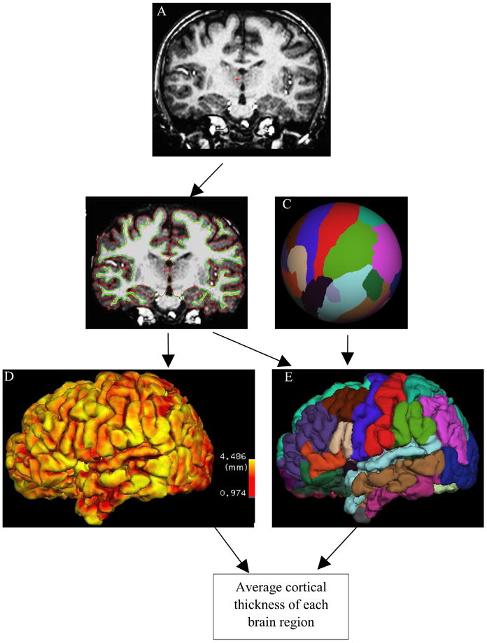
Surface-based analysis. A) T1 MR for a representative subject. B) Surfaces between white matter and gray matter (green line), and between gray matter and pial (red line), are overlaid on skull-stripped brain. C) Manually labeled cortical regions are mapped into a spherical space. D) Cortical thickness at each location of cortex. E) Surface-based labeling.

We used a cortical atlas that is based on statistics computed from manually labeled cortical regions; this atlas divides cerebral cortex (cerebellum and brain stem were removed and not analyzed in FreeSurfer) into 66 structures (33 structures for each hemisphere) (Desikan, et al. 2006). We mapped these structures onto a spherical space (Figure 2C) to achieve point-to-point correspondence for each subject (Fischl, et al. 2004). The final segmentation of surface-based labeling was based on both a subject-independent probabilistic atlas and on subject-specific measured values. Combining the cortical-thickness map (Figure 2D) and surface-based labels (Figure 2E), we computed the average cortical thickness for each cortical region.

We computed the volume of each structure as the average of the white-matter and pial surface areas, multiplied by the FreeSurfer-computed cortical thickness. The methods we used to compute cortical thicknesses and structure volumes were validated by Makris et al. (Makris, et al. 2006). VBM method for obtaining regional volumes and that used in FreeSurfer are different. In VBM, regional volumes are based on calculating numbers of voxels, whereas in surface-based methods, volumes are computed based on surface areas and thicknesses. FreeSurfer allows us to look at the two components of structure volumes (i.e., thickness and surface area) separately. Fischl et al. have found that these two components do not necessarily track one another (Fischl, et al. 1999); they therefore may yield additional information not available from volume measurements alone.

2.4 Data Analysis

A classification model includes two components: the structural form of the model, S, and model parameters, θ. We generated diagnostic models using WEKA (http://www.cs.waikato.ac.nz/ml/weka/), a widely used machine-learning software package (Witten and Frank 2005). We used the average thicknesses or volumes of brain structures as predictor variables. As described in the previous section, we divided the cerebral cortical surface into 66 regions, including both left and right hemispheres, according to surface-base labeling. The input data to the diagnostic-model–generation methods therefore consisted of 38 instances of 66 predictor variables with the group-membership variable assuming the label “ASD” or “VC”.

To avoid model-generation bias, we applied four machine-learning methods—support vector machines (SVMs), multilayer perceptrons (MLPs), functional trees (FTs), and logistic model trees (LMTs)—to generate diagnostic models. We selected SVMs (Platt 1999) because they have been shown empirically to achieve good generalization performance on a wide variety of classification problems (Sajda 2006). We selected MLPs because they represent a standard supervised-learning algorithm that can model nonlinear decision boundaries (Gardner and Dorling 1998). We selected both FT and LMT approaches because they can be seen as advanced versions of decision trees. The model generated by FT or LMT is declarative and simple to interpret, and more accurate than that generated by standard version decision trees, such as those generated by C4.5. FT is based on standard tree-based algorithms, such as CART and C4.5, yet FT has greater classification accuracy than these approaches (Gama 2004). LMT is based on the concept of a model tree, which is similar to an ordinary regression tree, except that it constructs a piecewise-linear, rather than a piecewise-constant, approximation to the target function; LMT builds a single tree containing only relevant attributes for classification, is more accurate than C4.5 and standalone logistic regression, and does not require tuning of parameters (Landwehr, et al. 2003).

We evaluated the diagnostic models generated by these four machine-learning algorithms based on 10-fold cross-validation; we randomly divided the data into 10 groups of 1 or 2 subjects each (i.e., one-tenth of subjects were placed in each group), with controls being mixed with ASD subjects. We ran 10 iterations, using 90% of subjects for classifier generation (i.e., training) and the remaining 10% for testing. After cycling through all 10 partitions for classification, every group was used for testing, and each group appeared in a training set every time except when it was used for testing.

We evaluated the performance of each diagnostic model based on the following metrics: true-positive rate, false-positive rate, accuracy, and area under the receiver operating characteristic (ROC) curve (AUC). Let N_TP denote the number of children with ASD correctly diagnosed as having ASD, N_FP denote the number of control subjects incorrectly identified as having ASD, N_TN denote the number of control subjects correctly identified, and N_FN denote children with ASD incorrectly identified as control subjects. Accuracy (ACC) is the proportion of correctly labeled instances in the study, defined as ACC = (N_TP + N_TN)/(N_TP + N_TN + N_FP + N_FN). The true-positive rate (TPR), or sensitivity, is the proportion of positive instances that were correctly reported as being positive (e.g. TPR = N_TP/(N_TP + N_FN)). The false-positive rate (FPR), or (1 – specificity), is the proportion of negative instances that were erroneously reported as being positive (FPR = N_FP/(N_FP + N_TN)). For a diagnostic system with probabilistic output, the ROC curve is a graphical plot of TPR (y-axis) against FPR (x-axis), as the discrimination threshold is varied. We used AUC as an additional measure of classification performance.

2.5 Data-Mining Methods

In this section we provide an overview of how we generated diagnostic models using SVM, MLP, FT, and LMT.

In linear form, SVM is a discriminant that separates positive from negative data by constructing a hyperplane with maximum margin, which is defined by the distance from the hyperplane to the nearest of the positive and negative data points (Platt 1999; Sajda 2006). SMO (Sequential minimal optimization) is a fast algorithm for training support vector machines (SVMs) (Platt 1999); SMO efficiently solves the dual optimization problem during derivation of the SVM, and improves scaling and computation time significantly (Platt 1999). We optimized SVM parameters based on 5-fold cross-validation. Because standard SVM classifiers cannot generate probability estimates, there is only one point on the ROC curve for SVM.

A MLP maps inputs onto a set of appropriate outputs using a feed-forward artificial neural-network model. A MLP uses three or more layers of nodes with nonlinear activation functions, and is thus more powerful than the standard linear perceptron for modeling nonlinear decision boundaries. MLP parameters are typically optimized based on internal cross-validation; we also optimized MLP parameters using this approach. MLPs have been shown to be useful for prediction and classification (Gardner and Dorling 1998).

A general framework for generating FTs is based on multivariate classification or regression trees using combinations of attributes at decision nodes, leaf nodes, or both (Gama 2004; Landwehr, et al. 2005). This method can accommodate binary and multi-class target variables, numeric and nominal predictor variables, and missing values. A decision tree can be constructed by a top-down recursive partitioning strategy: new attributes are constructed and mapped using a function such as multiple linear regression or multiple logistic regression. The merit of each new attribute is evaluated using the merit function of the univariate tree, in competition with the original attributes. The resulting model has two types of decision nodes: those based on a test of one of the original attributes, and those based on the values of the constructor function.

Classification of new subjects (i.e., those not used to generate the classifier) using a FT is accomplished by traversing the tree from the root node to a leaf node. At each decision node, the set of attributes is evaluated by the local constructor function, and the subject to be classified follows the path determined by the decision test (there was no missing value problem in our studies). When a leaf node is reached, the instance is classified using either the constant or the constructor function at that leaf.

A model tree is similar to an ordinary regression tree, except that it constructs a piecewise-linear (rather than a piecewise-constant) approximation to the target function. Logistic regression is a generalized linear model used for binomial regression. Combining a decision tree with logistic-regression models, a LMT classifier may consist of any combination of binary decisions based on numeric attributes, n-ary decisions based on nominal attributes, and logistic-regression models at leaf nodes (Landwehr, et al. 2003; Landwehr, et al. 2005).

LMT generation begins by constructing a logistic model at the root using the LogitBoost algorithm to iteratively fit simple linear-regression functions (Landwehr, et al. 2005). LogitBoost uses simple regression functions as base functions, and performs forward stage-wise fitting of additive symmetric logistic-regression models, based on maximum-likelihood calculations (Friedman, et al. 2000) and the C4.5 splitting criterion (Sumner, et al. 2005), thereby selecting variables that best predict the target variable. The LMT model is then extended at child nodes by using LogitBoost. Splitting at a node continues in this fashion until no additional useful split can be found. The LMT tree is then pruned using the CART cross-validation-based pruning algorithm.

2.6 Correlation between discriminant results and diagnostic criteria

To investigate the relationship between discriminant results and current autism symptoms, we computed correlation coefficients between LMT coefficients and ADI-R and CARS scores. Because ADI-R and CARS assessments were performed for only the ASD group, we could not compute correlation statistics for the VC group. For LMT, the model weight (w_i) for a subject can be obtained as follows (Landwehr, et al. 2003): $w_i=-log(\frac{1}{P_i}-1)$, where P_i is the probability that the i^th subject has ASD. For the ASD group, we computed Pearson product moment correlation coefficients between the weights (w_i), and ADI-R scores and CARS scores.

3. Results

Table 1 lists demographic characteristics of subjects in the ASD and VC groups. We did not find significant differences between groups in gender (chi-square p-value = 0.67), age (t-test p-value = 0.25), WISC full-scale IQ (t-test p-value = 0.44), weight (t-test p-value = 0.12), or height (t-test p-value = 0.16).

Table 1.

Subjects’ demographic variables

	ASD	VC	p-value1
Number of subjects	22	16	NA
Gender (male: female)	19:3	13:3	0.67
Handedness (right: left)	22:0	16:0	NA
Age (yrs)	9.2 ± 2.1	10.0 ± 1.9	0.25
Weight (kg)	30.6 ± 8.6	34.9 ± 8.2	0.12
Height (cm)	132.5 ± 12.1	138.6 ± 13.2	0.16
WISC-II FSIQ2	102.0 ± 22.4	107.5 ± 20.7	0.44
ADI-R Social3	18 ± 7	NA	NA
ADI-R Communication3	13 ± 5	NA	NA
ADI-R Behavior3	6 ± 3	NA	NA
CARS4	32 ± 5	NA	NA

¹p-value for gender using chi-square test; others p-values for the comparison between autism and control subjects are based on two-sample t-tests.

²Based on the Wechsler Intelligence Scale for Children-II (Chinese Version).

³Based on the Autism Diagnostic Inventory-Revised (ADI-R).

⁴Based on the Childhood Autism Rating Scale (CARS).

Tables 2A and 2B list classification performance metrics of the four diagnostic models for cortical regional thicknesses, and regional volumes, respectively. Figures 3A and 3B show the ROC curves of the four diagnostic models for thickness-based classification, and for volume-based classification, respectively. We compared the performance metrics of thickness-based and volume-based classification using the pairwise two-sample t statistic. P-values for accuracy, sensitivity, specificity, and AUC were 0.0003, 0.014, 0.0018, and 0.04, respectively. Thus, there were significant differences between the classification performance metrics of surface-based classifiers and those of volume-based classifiers: thickness-based classifiers outperformed volume-based classifiers.

Table 2.

A) Performance metrics for thickness-based classification;
	Accuracy (%)	TPR (Sensitivity)	FPR (1 - Specificity)	AUC
SVM (Thickness)	82	0.82	0.19	NA
MLP (Thickness)	82	0.82	0.19	0.82
FT (Thickness)	84	0.86	0.19	0.89
LMT (Thickness)	87	0.95	0.25	0.93

B) Performance metrics for volume-based classification.
	Accuracy (%)	TPR (Sensitivity)	FPR (1 - Specificity)	AUC
SVM (volume)	71	0.77	0.38	NA
MLP (volume)	71	0.73	0.31	0.76
FT (volume)	74	0.73	0.31	0.80
LMT (volume)	74	0.77	0.31	0.77

Figure 3.

A) ROC curves for LMT, FT, and MLP classifiers for thickness-based classification; B) ROC curves of LMT, FT, and MLP classifiers for volume-based classification. Note that SVM has only one point on the ROC plot because SVM cannot generate probability estimates.

For thickness-based classification, the SVM and MLP approaches used all 66 predictor variables in the classification model, whereas FT selected 12 predictor variables, and LMT generated the simplest model, with seven predictor variables (Table 3 and Figure 4). All seven structures selected by LMT were included in the set of structures selected by FT.

Table 3.

Average thickness of structures selected by LMT for thickness-based classification, and two-sample t-test p-values (not adjusted for multiple comparisons) to determine whether significant differences exist between groups.

Predictor Variables	ASD (mm)	VC (mm)	p-value
Right pars triangularis	2.61 ± 0.15	2.82 ± 0.21	0.002
Left caudal anterior cingulate	3.15 ± 0.41	2.75 ± 0.40	0.005
Left medial orbitofrontal	2.64 ± 0.21	3.01 ± 0.26	< 0.0001
Left parahippocampal	2.08 ± 0.33	2.33 ± 0.34	0.03
Left pars triangularis	2.64 ± 0.19	2.82 ± 0.22	0.01
Left precuneus	2.74 ± 0.13	2.64 ± 0.15	0.04
Left frontal pole	3.38 ± 0.49	3.73 ± 0.27	0.008

Figure 4.

The seven structures selected by LMT. The blue ROIs represent regions for which cortex was thinner in the ASD group (we color the frontal pole in dark blue, because it is contiguous with medial orbitofrontal cortex), and red ROIs represent regions for which cortex was thicker in the ASD group.

We computed the two-sample t statistic to determine whether the average cortical thicknesses of the seven structures in the LMT diagnostic model differed across groups. We found that cortex in the right pars triangularis (p-value = 0.002), left medial orbitofrontal gyrus (p-value < 0.0001), left parahippocampal gyrus (p-value = 0.03), left pars triangularis (p-value = 0.01), and left frontal pole (p-value = 0.008) was thinner in ASD than in VC subjects, whereas cortex in the left caudal anterior cingulate (p-value = 0.005) and left precuneus (p-value = 0.04) was thicker in ASD subjects.

Table 5 shows regions manifesting significant differences between ASD and VC subjects for thickness- (Table 5A) and volume-based (Table 5B) methods. We found 17 structures with significant differences between groups for thickness-based analysis (p-value < 0.05, uncorrected for multiple comparisons), and nine regions with significant differences for volume-based analysis (p-value < 0.05, uncorrected for multiple comparisons). For multiple comparison correction, we adjusted these t-test p-values to achieve a false discovery rate (FDR) q < 0.05 (marked with “**”) (Benjamini and Hochberg, 1995). We found 8 structures with significant differences between groups for thickness-based analysis (q < 0.05), and no regions with significant differences for volume-based analysis (q < 0.05).

Table 5.

Regions manifesting significant thickness or volume differences between ASD and VC groups.

A) Thickness-based
Regions1	ASD (mm)	VC (mm)	p-value2
R entorhinal	2.37 ± 0.38	2.87 ± 0.60	0.008**
L entorhinal	2.46 ± 0.50	2.83 ± 0.52	0.04
R lateral orbitofrontal	2.65 ± 0.23	2.91 ± 0.20	0.0006**
L lateral orbitofrontal	2.71 ± 0.25	2.95 ± 0.14	0.0005**
R medial orbitofrontal	2.49 ± 0.29	2.86 ± 0.34	0.001**
L medial orbitofrontal *	2.64 ± 0.21	3.01 ± 0.26	< 0.0001**
R parahippocampal	2.03 ± 0.26	2.24 ± 0.23	0.01
L parahippocampal *	2.08±0.33	2.33 ± 0.34	0.03
R pars triangularis *	2.61 ± 0.15	2.82 ± 0.21	0.002**
L pars triangularis*	2.64 ± 0.19	2.82 ± 0.22	0.01
R temporal pole	2.67 ± 0.53	3.07 ± 0.54	0.03
L temporal pole	2.77 ± 0.61	3.21 ± 0.52	0.02
R rostral middle frontal	2.66 ± 0.15	2.76 ± 0.10	0.03
L caudal anterior cingulated*	3.15 ± 0.41	2.75 ± 0.40	0.004**
L precuneus *	2.74 ± 0.13	2.64 ± 0.15	0.04
L superior parietal	2.63 ± 0.19	2.51 ± 0.15	0.05
L frontal pole *	3.38 ± 0.49	3.73 ± 0.27	0.008**

B) Volume-based
Regions1	ASD(mm3)	VC(mm3)	p- value2
R entorhinal	1135 ± 345	1496 ± 515	0.02
L entorhinal	1091 ± 476	1471 ± 448	0.02
R medial orbitofrontal	4264 ± 861	5369 ± 1126	0.003
L medial orbitofrontal	4454 ± 859	5319 ± 928	0.006
R lateral orbitofrontal	6771 ± 1623	7881 ± 1316	0.03
R temporal pole	1424 ± 654	1971 ± 651	0.02
L caudal anterior cingulate	1860 ± 558	1388 ± 259	0.001
L parahippocampal	1719 ± 322	1979 ± 385	0.04
L frontal pole	1220 ± 337	1543 ± 421	0.02

¹Regions marked with “*” were predictor variables chosen by LMT. L: left hemisphere; R: right hemisphere.

²Two-sample t-test. P-values marked with “**” were significant at false discovery rate (FDR) q < 0.05 (Benjamini and Hochberg, 1995).

¹All regions that were found to be significantly different with respect to volume were also found to be significantly different with respect to thickness. L: left hemisphere; R: right hemisphere.

²Two-sample t-test. None was chosen using false discovery rate (FDR) q < 0.05 (Benjamini and Hochberg, 1995).

Table 6 lists correlation coefficients between diagnostic criteria and LMT model weights, for both thickness- and volume-based methods. Figure 5 shows the correlation plots for clinical diagnostic criteria (ADI-R and CARS) and LMT thickness-based model weights. The thickness-based model weights were positively but not significantly correlated with test scores. The volume-based model weights were negatively correlated with ADI-R social, ADI-R communication, and CARS score, and positively correlated with ADI-R behavior, but none of these correlations were significant.

Table 6.

Correlation coefficients between diagnostic criteria and the weights of predictor variables chosen by LMT (r: correlation coefficient, p: p-value).

Diagnostic test	Thickness- based		Volumes-based
	r	p	r	p
ADI-R Social	0.22	0.35	−0.048	0.84
ADI-R Communication	0.11	0.63	−0.018	0.94
ADI-R Behavior	0.36	0.14	0.33	0.14
CARS	0.23	0.31	−0.012	0.96

Figure 5.

Correlation plots for clinical diagnostic criteria (ADI-R and CARS) and LMT thickness-based model weights (r: correlation coefficient).

4. Discussion

To our knowledge, there has been no previous attempt to compare thickness and volume-based classification of ASD. We found that thickness-based classification was more accurate than volume-based classification, for each combination of classifier and performance metric.

We used four machine-learning methods to generate classifiers, in order to avoid bias with respect to the functional form of the classifier. The results listed in Table 2 suggest that: 1) SVM and MLP have similar performance, and LMT and FT have similar performance. This is expected, since both SVM and MLP are margin-based, and LMT and FT are tree-based. 2) FT and LMT perform only modestly better than SVM and MLP. 3) LMT and FT can generate declarative models that are easy to interpret, and have effective feature-selection mechanisms. SVM and MLP are so-called “black-box” approaches: they do not generate declarative models. 4) LMT and FT generate models with similar neuroanatomic markers. FT includes several structures in addition to those selected by LMT.

Previous studies have reported that LMT models classify more accurately than those generated by FT (Landwehr, et al. 2005); other researchers have found that LMT has performance similar to that of SVM, but better than that of MLP (Aires, et al. 2004; Petrova, et al. 2006); yet other researchers found that LMT’s performance is only slightly better than that of SVM (Altmann, et al, 2007). All of these results were based on a larger sample size than ours. Among thickness-based diagnostic models, the diagnostic model generated by LMT achieved the best classification performance; this model included seven structures. For these seven structures, relative to controls, cortical thickness in the ASD group was significantly thinner in the right pars triangularis, left medial orbitofrontal gyrus, left parahippocampal gyrus, left pars triangularis and left frontal pole, but thicker in the left caudal anterior cingulate gyrus and in left precuneus (Table 3).

Of the regions manifesting relatively thinner cortex in the ASD group (blue ROIs in Figure 4), pars triangularis (Brodmann area 45) is a region within Broca’s area, in the inferior frontal gyrus, and is thought to contribute to language comprehension and social impairment (Amaral, et al. 2008). The medial orbitofrontal region is involved in decision-making and expectation regarding the value of reinforcement, and in sensory integration (Kringelbach 2005). The parahippocampal gyrus contributes to understanding of the interactions between emotion and cognition, and may be associated with reactivation of contextual fear memory that results in avoidance behavior (Ke, et al. 2008). The frontal pole plays a role in retrospective memory and in higher-order cognitive operations (e.g., decision making, planning, and social and moral reasoning) (Okuda, et al. 2003).

Regarding the relatively thicker regions in the ASD group (red ROIs in Figure 4), the precuneus is involved in visuospatial imagery, episodic memory retrieval and self-processing operations (Cavanna and Trimble 2006). The caudal anterior cingulate is associated with the cognitive control of behavior, and is involved in load and performance monitoring for working memory (Gray and Braver 2002; Ursu, et al. 2009).

Hardan et al. reported that parietal cortex had increased cortical thickness in an autism group (Hardan, et al. 2006). Similarly, we found that the left precuneus, which is in the parietal lobe, manifested increased cortical thickness in the ASD group.

A few postmortem studies have been published on the neuropathology of autism. Kemper and Bauman (Kemper and Bauman 1993) found the caudal anterior cingulate appeared unusually coarse in a study that included six cases of autism. In our studies, the left caudal anterior cingulate manifested increased cortical thickness in the ASD group. Autism researchers have found reduced cortical thickness in the inferior frontal gyrus, the orbitofrontal region, the temporal region and the prefrontal region bilaterally (Hadjikhani, et al. 2006); there has also been a report of decreased gray-matter volume in the right parahippocampal gyrus (Ke, et al. 2008). We found similar cortical thinning in autistic subjects: bilateral pars triangularis (which is in the inferior frontal gyrus), left medial orbitofrontal region (which is within the orbitofrontal region), left frontal pole (which is within the prefrontal region), and left parahippocampal gyrus (which is within the temporal region).

Abnormalities of the brain regions found in our analysis can be implicated in three core behaviors that are impaired in autism (Amaral, et al. 2008): social behavior (pars triangularis, medial orbitofrontal region, caudal anterior cingulate), language and communication (pars triangularis), and repetitive and stereotyped behavior (medial orbitofrontal region, caudal anterior cingulate). In addition, cortical thinning in the left parahippocampal gyrus may contribute to the neural basis for ignoring dangers in autistic children (Ke, et al. 2008).

Many neuroanatomical abnormalities of the cerebral cortex have been reported in autism studies, using a broad range of analytic methods. Several VBM studies have identified significant differences between autistic and control subjects in frontal lobes, parietal lobes, temporal lobes (Aylward, et al. 2002; Aylward, et al. 1999; Ke, et al. 2008; Rojas, et al. 2006), as we found in our analysis.

There have also been several previous SBM studies of autism. Hadjikhani et al. (Hadjikhani, et al. 2007) found anatomical differences in the mirror-neuron system in and other areas involved in social cognition in individuals with ASD using SBM. They detected regions similar to ours, including bilateral pars triangularis, both orbitofrontal regions, both temporal regions and both prefrontal regions. Nordahl et al. (Nordahl, et al. 2007) employed SBM to detect cortical-folding (rather than cortical-thickness) abnormalities in autism; results included left operculum, bilateral parietal operculum, and bilateral intraparietal sulcus. These two studies did not construct classification models from structures that they found to differ between groups.

Note that the neuroanatomical markers for ASD that we detected with LMT may not be consistent with those found in some previous studies (Amaral, et al. 2008; Aylward, et al. 2002; Aylward, et al. 1999; Ke, et al. 2008; Hadjikhani, et al. 2006; Nordahl, et al. 2007; Rojas, et al. 2006) that centered on the detection of regions demonstrating volumetric or thickness differences between autistic and control subjects. Several potential reasons for these discrepancies include: 1) our neuroanatomical markers for ASD were detected based on their contribution to classification. However, several regions may make similar contributions to classification, and feature selection will, in general, choose only one of a set of similar regions to include in a classification model. In addition, there may exist structures demonstrating significant volumetric or thickness differences between groups, yet these structures may contribute little to classification. For example, Table 5 lists 17 regions that demonstrate significant thickness differences across groups, yet LMT included only 7 of these 17 variables in its classification model. 2) Different study populations, ages, and genders (please see Appendix 3 for consideration of possible gender effect), clinical and MR instruments, image-processing algorithms, and brain atlases, among other differences, will also contribute to different results.

The differences between our volume-based analysis and that performed by Ecker et al. (Ecker, et al. 2009) are as follows. First, our image-preprocessing pipelines (including image segmentation and registration) were different. Ecker et al. used unified segmentation in SPM5: each image was normalized into the MNI atlas space, and segmented into GM, WM and CSF; then, each GM voxel was used as a candidate predictor variable in their model. Our volume-based analysis is atlas-based, and includes 66 candidate predictor variables (based on the FreeSurfer atlas). Second, Ecker’s study included subcortical regions such as the amygdala, which may play important roles in ASD; surface-based methods cannot analyze subcortical structures. Third, FreeSurfer uses cortical geometry to perform inter-subject registration, which results in a much better matching of homologous cortical regions than volumetric techniques (Fischl, et al. 1999). These differences render the results of Ecker’s and these of our volume-based SVM approaches difficult to compare.

To make our results more comparable, we followed Ecker’s approach to VBM classification (see Appendix 1), and obtained accuracy results that were similar to those obtained from our original volume-based classification. In particular, the performance of VBM classification following Ecker’s approach was not as good as than that of thickness-based classification, for our subjects.

The volume-based predictor variables selected by LMT are shown in Table 4. Half of our volume-based predictor variables were also reported as predictor variables in (Ecker, et al. 2009), and one quarter were also selected by the thickness-based approach. In order to determine whether thickness-based features were more important than volume-based features, we combined the thickness- and volume-based features for machine learning (Appendix 2). We found the volume-based features were less important than the thickness-based features in the tree-based model; that is, the machine-learning algorithms chose thickness-based features rather than volume-based features in generating classification models.

Table 4.

Volume-based predictor variables

Volume-based predictor variable
R inferior parietal cortex *
R precuneus cortex *
R superior temporal gyrus *
L superior temporal sulcus *
L fusiform gyrus *
L posterior-cingulate cortex *
L precuneus cortex *
L caudal middle frontal gyrus *
L caudal anterior cingulate cortex
L medial orbitofrontal cortex
L pars triangularis
R rostral anterior cingulate cortex
R medial orbitofrontal cortex
L paracentral lobule
L supramarginal gyrus
L cuneus cortex

[1] L: left hemisphere; R: right hemisphere.

[2] Regions marked with “*” are also reported as predictor variables in (Ecker, et al. 2009)

[3] Regions in italics were also found by thickness-based classification.

For either thickness- or volume-based analysis, we found no significant correlation between model weights (defined in Section 2.6), and CARS or any of the three ADI-R sub-scores. Similarly, Ecker et al. found no significant correlation between model weights and CARS or the ADI-R sub-scores (Ecker, et al. 2009). Lack of significant correlation between the model weights and CARS or ADI sub-scores highlights differences between behavioral assessment and morphology-based classification, and indicates that theses approaches may be complementary in assessing children for ASD.

Of note, we have not sought through these analyses to develop classifiers that would replace behavioral testing for the diagnosis of ASD. We believe that the benefits of these diagnostic models are twofold. First, these classifiers could provide neuroanatomic markers (e.g., the seven regions detected by LMT) for subsequent investigation. Second, these MR-based classifiers may provide information (a neuroanatomic foundation for ASD) that is complementary to that obtained by behavioral assessment. The potential contributions of MR-based diagnostic aides were also described by Ecker et al. (Ecker, et al. 2009).

One of the limitations of this study is the small sample sizes of both the ASD and VC groups. Small sample size leads to decreased precision in estimates of various properties of the population, adversely influences diagnostic-model generation and testing, and makes performance estimation of diagnostic models difficult. Thus, we might find that increasing sample size would lead us to change our opinions about the relative merits of the four machine-learning approaches that we applied. Cross-validation only partly alleviates the error-estimation problem; it is known to overestimate classification accuracy. Although other machine-learning researchers have used cross validation with similar sample sizes (e.g., Ecker, et al. 2009; Kloppel, et al. 2008; Singh, et al. 2008), the ultimate way to refine classification models, and to verify these results, is to increase sample size. We plan to accrue additional subjects, and to repeat these analyses (and thereby refine our classification models) as our sample sizes increase.

Another limitation of our surface-based approach is its inability to admit subcortical structures, such as the amygdala and the basal ganglia, which may play crucial roles in ASD (Hadjikhani, et al. 2006). To remedy this limitation, we plan to develop hybrid classification models that include surface-based and volume-based features.

Image quality may be another limitation of any MR-based analysis. We excluded subjects with poor MR image quality, and all MR images were reviewed by an experienced radiologist for quality. We also used FreeSurfer (Dale, et al. 1999; Fischl, et al. 1999) to correct for motion. We would expect that the noise introduced by poor image quality would cause our algorithms to find few or no features that distinguish ASD from control subjects, and that the resulting models would manifest poor classification performance, which was not the case.

We believe that we will obtain more accurate and stable classifiers by enhancing the set of morphological attributes that we present to the data-mining algorithms. For example, with respect to surface-based analysis, we will compute additional attributes, such as mean curvature, Gaussian curvature, folding index, and curvature index (details are presented in Makris, et al. 2006). Another promising avenue for expanding our candidate feature set is to include the results of autism-related genetic tests (Cheng, et al. 2009). Finally, we plan to develop voxel-based analyses, to complement the information gained from analyses based on surface and volumetric features of atlas structures.

Other applications of SBM include studies of Alzheimer disease (Bakkour, et al. 2009; Dickerson, et al. 2009) and schizophrenia (Shen, et al. 2004).

5. Conclusion

To our knowledge, this study represents the first attempt to classify autism using regional cortical thickness measurements extracted from SBM, and to compare classification results to those obtained from volume-based analysis. The principal contribution of our work is our determination that thickness-based classification results in significantly more accurate classification than volume-based classification, across four different classification approaches, and four classification-accuracy metrics. The machine-learning approach that performed best, LMT, generated a simple and declarative diagnostic model based on seven neuroanatomical markers. Our results suggest that cortical thickness may be more strongly predictive of ASD and reflect more intrinsic topology of cortex than the more widely used volume-based features.

Abbreviations

ASD

autism spectrum disorder

SBM

surface-based morphometry

VBM

voxel-based morphometry

VC

volunteer controls

DSM-IV

the fourth edition of Diagnostic and Statistical Manual of Mental Disorders

ADI-R

Autism Diagnostic Inventory-Revised

CARS

Childhood Autism Rating Scale

MR

magnetic resonance

SVM

Support Vector Machines

MLP

Multilayer Perceptron

FT

Fictional Tree

LMT

Logistic Model Tree

ACC

accuracy

ROC

receiver operating characteristic

AUC

area under the ROC curve

TPR

true positive rate

FPR

false positive rare

ROI

region of interest

Appendix 1: Classification based on Ecker’s approach

Following Ecker’s methods (Ecker, et al. 2009) of image processing (SPM5) and classification methods (SVM classification implemented by LibSVM (http://www.csie.ntu.edu.tw/~cjlin/libsvm/)), we supplied GM images as predictor variables and obtained VBM-based classification accuracy of 71%, using 10-fold cross-validation. Our VBM classification was not similar to that of Ecker’s group, possibly due to different study populations and MR instruments.

For our study population, the performance of VBM classification was worse than that of thickness-based. VBM classification accuracy was 71%, while thickness-based accuracy with SMO as the classifier was 82%.

Appendix 2: Classification based on a combination of thickness- and volume-based features

In order to determine whether thickness-based features are more important than the volume-based features for constructing accurate classifiers, we combined the thickness- and volume-based features together into a single training data set. Accuracies for SVM, MLP, FT, and LMT were 71%, 76%, 84%, and 78%.

For tree-based methods, FT chose 8 thickness-based features and 4 volume-based features, and LMT chose 12 thickness feature and 10 volume features. The average contribution weights of thickness-based features for FT and LMT were 2.56, and 2.90, respectively. However, the average contribution weights of volume-based features for both FT and LMT were approximate 0, much smaller than those of the thickness-based features.

Appendix 3: Assessment of gender effect

Previous studies have demonstrated that brain development during childhood and adolescence is sexually dimorphic (Lenroot et al. 2007). To investigate gender effect in our analyses, we added gender as a predictor variable with states M (male) and F (female). We found that FT and LMT did not select gender as a prediction model variable for either thickness- or volume-based analysis, and that classification performance (Table 7) was almost identical to results obtained without including the gender variable. Therefore, in our studies, gender did not appear to be a factor for classification, although this finding may well be due to inadequate statistical power (i.e., small numbers of male and female subjects).

Table 7.

Classification performance when gender is included in the analysis.

A) Accuracy, TPR, FPR, and AUC for thickness-based classification.
Thickness-based	Accuracy (%)	TPR	FPR	AUC
SVM	76	0.77	0.25	NA
MLP	79	0.77	0.19	0.80
FT	84	0.86	0.19	0.89
LMT	84	0.91	0.25	0.93

B) Accuracy, TPR, FPR, and AUC for volume-based classification.
Volume-based	Accuracy (%)	TPR	FPR	AUC
SVM	71	0.73	0.31	NA
MLP	68	0.73	0.38	0.78
FT	71	0.73	0.31	0.81
LMT	71	0.77	0.38	0.78

References

- Akshoomoff N, Lord C, Lincoln AJ, Courchesne RY, Carper RA, Townsend J, Courchesne E. Outcome classification of preschool children with autism spectrum disorders using MRI brain measures. J Am Acad Child Adolesc Psychiatry. 2004;43(3):349–57. doi: 10.1097/00004583-200403000-00018. [DOI] [PubMed] [Google Scholar]
- Altmann A, Beerenwinkel N, et al. Improved prediction of response to antiretroviral combination therapy using the genetic barrier to drug resistance. Antivir Ther. 2007;12(2):169–78. doi: 10.1177/135965350701200202. [DOI] [PubMed] [Google Scholar]
- Amaral DG, Schumann CM, Nordahl CW. Neuroanatomy of autism. Trends in Neurosciences. 2008;31(3):137–145. doi: 10.1016/j.tins.2007.12.005. [DOI] [PubMed] [Google Scholar]
- Aires R, Manfrin A, Aluisio S, Santos D. Technical Report NILC-TR-04-09. Brasil: University de Sao Paulo; 2004. Which classification algorithm works best with stylistic features of Portuguese in order to classify web texts according to users needs? [Google Scholar]
- Aylward EH, Minshew NJ, Field K, Sparks BF, Singh N. Effects of age on brain volume and head circumference in autism. Neurology. 2002;59(2):175–83. doi: 10.1212/wnl.59.2.175. [DOI] [PubMed] [Google Scholar]
- Aylward EH, Minshew NJ, Goldstein G, Honeycutt NA, Augustine AM, Yates KO, Barta PE, Pearlson GD. MRI volumes of amygdala and hippocampus in non-mentally retarded autistic adolescents and adults. Neurology. 1999;53(9):2145–50. doi: 10.1212/wnl.53.9.2145. [DOI] [PubMed] [Google Scholar]
- Bakkour A, Morris JC, Dickerson BC. The cortical signature of prodromal AD: regional thinning predicts mild AD dementia. Neurology. 2009;72(12):1048–55. doi: 10.1212/01.wnl.0000340981.97664.2f. [DOI] [PMC free article] [PubMed] [Google Scholar]
- Belmonte MK, Cook EH, Anderson GM, Rubenstein JLR, Greenough WT, Beckel-Mitchener A, Courchesne E, Boulanger LM, Powell SB, Levitt PR, et al. Autism as a disorder of neural information processing: directions for research and targets for therapy. Molecular Psychiatry. 2004;9(7):646–663. doi: 10.1038/sj.mp.4001499. [DOI] [PubMed] [Google Scholar]
- Benjamini Yoav, Hochberg Yosef. Controlling the false discovery rate: a practical and powerful approach to multiple testing. Journal of the Royal Statistical Society, Series B (Methodological) 1995;57 (1):289–300. [Google Scholar]
- Cavanna AE, Trimble MR. The precuneus: a review of its functional anatomy and behavioural correlates. Brain. 2006;129(Pt 3):564–83. doi: 10.1093/brain/awl004. [DOI] [PubMed] [Google Scholar]
- Cheng L, Ge Q, Xiao P, Sun B, Ke X, Bai Y, Lu Z. Association Study between BDNF Gene Polymorphisms and Autism by Three-Dimensional Gel-Based Microarray. Int J Mol Sci. 2009;10(6):2487–500. doi: 10.3390/ijms10062487. [DOI] [PMC free article] [PubMed] [Google Scholar]
- Courchesne E, Karns CM, Davis HR, Ziccardi R, Carper RA, Tigue ZD, Chisum HJ, Moses P, Pierce K, Lord C, et al. Unusual brain growth patterns in early life in patients with autistic disorder: an MRI study. Neurology. 2001;57(2):245–54. doi: 10.1212/wnl.57.2.245. [DOI] [PubMed] [Google Scholar]
- Dale AM, Fischl B, Sereno MI. Cortical surface-based analysis. I. Segmentation and surface reconstruction. Neuroimage. 1999;9(2):179–94. doi: 10.1006/nimg.1998.0395. [DOI] [PubMed] [Google Scholar]
- Desikan RS, Ségonne F, Fischl B, Quinn BT, Dickerson BC, Blacker D, Buckner RL, Dale AM, Maguire RP, Hyman BT, et al. An automated labeling system for subdividing the human cerebral cortex on MRI scans into gyral based regions of interest. NeuroImage. 2006;31(3):968–980. doi: 10.1016/j.neuroimage.2006.01.021. [DOI] [PubMed] [Google Scholar]
- Dickerson BC, Bakkour A, Salat DH, Feczko E, Pacheco J, Greve DN, Grodstein F, Wright CI, Blacker D, Rosas HD, et al. The Cortical Signature of Alzheimer’s Disease: Regionally Specific Cortical Thinning Relates to Symptom Severity in Very Mild to Mild AD Dementia and is Detectable in Asymptomatic Amyloid-Positive Individuals 10.1093/cercor/bhn113. Cereb Cortex. 2009;19(3):497–510. doi: 10.1093/cercor/bhn113. [DOI] [PMC free article] [PubMed] [Google Scholar]
- Ecker C, Rocha-Rego V, Johnston P, Mourao-Miranda J, Marquand A, Daly EM, Brammer MJ, Murphy C, Murphy DG. Investigating the predictive value of whole-brain structural MR scans in autism: A pattern classification approach. Neuroimage. 2009 doi: 10.1016/j.neuroimage.2009.08.024. [DOI] [PubMed] [Google Scholar]
- Fischl B, Dale AM. Measuring the thickness of the human cerebral cortex from magnetic resonance images. Proceedings of the National Academy of Sciences of the United States of America. 2000;97(20):11050–11055. doi: 10.1073/pnas.200033797. [DOI] [PMC free article] [PubMed] [Google Scholar]
- Fischl B, Sereno MI, Dale AM. Cortical surface-based analysis. II: Inflation, flattening, and a surface-based coordinate system. Neuroimage. 1999;9(2):195–207. doi: 10.1006/nimg.1998.0396. [DOI] [PubMed] [Google Scholar]
- Fischl B, van der Kouwe A, Destrieux C, Halgren E, Segonne F, Salat DH, Busa E, Seidman LJ, Goldstein J, Kennedy D, et al. Automatically parcellating the human cerebral cortex. Cereb Cortex. 2004;14(1):11–22. doi: 10.1093/cercor/bhg087. [DOI] [PubMed] [Google Scholar]
- Friedman J, Hastie T, Tibshirani R. Additive logistic regression: A statistical view of boosting. Annals of Statistics. 2000;28(2):337–374. [Google Scholar]
- Gama J. Functional trees. Machine Learning. 2004;55(3):219–250. [Google Scholar]
- Gardner MW, Dorling SR. Artificial neural networks (the multilayer perceptron)--a review of applications in the atmospheric sciences. Atmospheric Environment. 1998;32(14–15):2627–2636. [Google Scholar]
- Geschwind DH. Advances in Autism. Annu Rev Med. 2009;60:367–380. doi: 10.1146/annurev.med.60.053107.121225. [DOI] [PMC free article] [PubMed] [Google Scholar]
- Gmitrowicz A, Kucharska A. Developmental disorders in the fourth edition of the American classification: diagnostic and statistical manual of mental disorders (DSM IV -- optional book) Psychiatr Pol. 1994;28(5):509–21. [PubMed] [Google Scholar]
- Gray JR, Braver TS. Personality predicts working-memory-related activation in the caudal anterior cingulate cortex. Cogn Affect Behav Neurosci. 2002;2(1):64–75. doi: 10.3758/cabn.2.1.64. [DOI] [PubMed] [Google Scholar]
- Hadjikhani N, Joseph RM, Snyder J, Tager-Flusberg H. Anatomical differences in the mirror neuron system and social cognition network in autism. Cereb Cortex. 2006;16(9):1276–82. doi: 10.1093/cercor/bhj069. [DOI] [PubMed] [Google Scholar]
- Hadjikhani N, Joseph RM, Snyder J, Tager-Flusberg H. Abnormal activation of the social brain during face perception in autism. Human Brain Mapping. 2007;28(5):441–449. doi: 10.1002/hbm.20283. [DOI] [PMC free article] [PubMed] [Google Scholar]
- Han X, Jovicich J, Salat D, van der Kouwe A, Quinn B, Czanner S, Busa E, Pacheco J, Albert M, Killiany R, et al. Reliability of MRI-derived measurements of human cerebral cortical thickness: the effects of field strength, scanner upgrade and manufacturer. Neuroimage. 2006;32(1):180–94. doi: 10.1016/j.neuroimage.2006.02.051. [DOI] [PubMed] [Google Scholar]
- Hardan AY, Muddasani S, Vemulapalli M, Keshavan MS, Minshew NJ. An MRI study of increased cortical thickness in autism. Am J Psychiatry. 2006;163(7):1290–2. doi: 10.1176/appi.ajp.163.7.1290. [DOI] [PMC free article] [PubMed] [Google Scholar]
- Hashimoto T, Tayama M, Murakawa K, Yoshimoto T, Miyazaki M, Harada M, Kuroda Y. Development of the brainstem and cerebellum in autistic patients. J Autism Dev Disord. 1995;25(1):1–18. doi: 10.1007/BF02178163. [DOI] [PubMed] [Google Scholar]
- Ke X, Hong S, Tang T, Zou B, Li H, Hang Y, Zhou Z, Ruan Z, Lu Z, Tao G, et al. Voxel-based morphometry study on brain structure in children with high-functioning autism. Neuroreport. 2008;19(9):921–5. doi: 10.1097/WNR.0b013e328300edf3. [DOI] [PubMed] [Google Scholar]
- Kemper TL, Bauman ML. The contribution of neuropathologic studies to the understanding of autism. Neurol Clin. 1993;11(1):175–87. [PubMed] [Google Scholar]
- Kim JS, Singh V, Lee JK, Lerch J, Ad-Dab’bagh Y, MacDonald D, Lee JM, Kim SI, Evans AC. Automated 3-D extraction and evaluation of the inner and outer cortical surfaces using a Laplacian map and partial volume effect classification. Neuroimage. 2005;27(1):210–221. doi: 10.1016/j.neuroimage.2005.03.036. [DOI] [PubMed] [Google Scholar]
- Kirk GR, Haynes MR, Palasis S, Brown C, Burns TG, McCormick M, Jones RA. Regionally specific cortical thinning in children with sickle cell disease. Cereb Cortex. 2009;19(7):1549–56. doi: 10.1093/cercor/bhn193. [DOI] [PubMed] [Google Scholar]
- Kloppel S, Stonnington CM, Chu C, Draganski B, Scahill RI, Rohrer JD, Fox NC, Jack CR, Jr, Ashburner J, Frackowiak RS. Automatic classification of MR scans in Alzheimer’s disease. Brain. 2008;131(Pt 3):681–9. doi: 10.1093/brain/awm319. [DOI] [PMC free article] [PubMed] [Google Scholar]
- Kringelbach ML. The human orbitofrontal cortex: linking reward to hedonic experience. Nat Rev Neurosci. 2005;6(9):691–702. doi: 10.1038/nrn1747. [DOI] [PubMed] [Google Scholar]
- Landwehr N, Hall M, Frank E. Logistic model trees. Machine Learning: Ecml 2003. 2003;2837:241–252. [Google Scholar]
- Landwehr N, Hall M, Frank E. Logistic model trees. Machine Learning. 2005;59(1–2):161–205. [Google Scholar]
- Lenroot RK, Gogtay N, Greenstein DK, Wells EM, Wallace GL, Clasen LS, Blumenthal JD, Lerch J, Zijdenbos AP, Evans AC, et al. Sexual dimorphism of brain developmental trajectories during childhood and adolescence. Neuroimage. 2007;36(4):1065–73. doi: 10.1016/j.neuroimage.2007.03.053. [DOI] [PMC free article] [PubMed] [Google Scholar]
- Lord C, Rutter M, Le Couteur A. Autism Diagnostic Interview-Revised: a revised version of a diagnostic interview for caregivers of individuals with possible pervasive developmental disorders. J Autism Dev Disord. 1994;24(5):659–85. doi: 10.1007/BF02172145. [DOI] [PubMed] [Google Scholar]
- Makris N, Kaiser J, Haselgrove C, Seidman LJ, Biederman J, Boriel D, Valera EM, Papadimitriou GM, Fischl B, Caviness VS, Jr, et al. Human cerebral cortex: a system for the integration of volume- and surface-based representations. Neuroimage. 2006;33(1):139–53. doi: 10.1016/j.neuroimage.2006.04.220. [DOI] [PubMed] [Google Scholar]
- Muller RA. The study of autism as a distributed disorder. Mental Retardation and Developmental Disabilities Research Reviews. 2007;13(1):85–95. doi: 10.1002/mrdd.20141. [DOI] [PMC free article] [PubMed] [Google Scholar]
- Nordahl CW, Dierker D, Mostafavi I, Schumann CM, Rivera SM, Amaral DG, Van Essen DC. Cortical folding abnormalities in autism revealed by surface-based morphometry. Journal of Neuroscience. 2007;27(43):11725–11735. doi: 10.1523/JNEUROSCI.0777-07.2007. [DOI] [PMC free article] [PubMed] [Google Scholar]
- Okuda J, Fujii T, Ohtake H, Tsukiura T, Tanji K, Suzuki K, Kawashima R, Fukuda H, Itoh M, Yamadori A. Thinking of the future and past: the roles of the frontal pole and the medial temporal lobes. NeuroImage. 2003;19(4):1369–1380. doi: 10.1016/s1053-8119(03)00179-4. [DOI] [PubMed] [Google Scholar]
- Petrova NV, Wu CH. Prediction of catalytic residues using Support Vector Machine with selected protein sequence and structural properties. BMC Bioinformatics. 2006;7:312. doi: 10.1186/1471-2105-7-312. [DOI] [PMC free article] [PubMed] [Google Scholar]
- Platt JC. Fast training of support vector machines using sequential minimal optimization Advances in kernel methods: support vector learning MIT Press. 1999:185–208. [Google Scholar]
- Rapin I. Autism. New England Journal of Medicine. 1997;337(2):97–104. doi: 10.1056/NEJM199707103370206. [DOI] [PubMed] [Google Scholar]
- Rojas DC, Peterson E, Winterrowd E, Reite ML, Rogers SJ, Tregellas JR. Regional gray matter volumetric changes in autism associated with social and repetitive behavior symptoms. BMC Psychiatry. 2006;6:56. doi: 10.1186/1471-244X-6-56. [DOI] [PMC free article] [PubMed] [Google Scholar]
- Sajda P. Machine learning for detection and diagnosis of disease. Annual Review of Biomedical Engineering. 2006;8:537–565. doi: 10.1146/annurev.bioeng.8.061505.095802. [DOI] [PubMed] [Google Scholar]
- Schopler E, Reichler RJ, DeVellis RF, Daly K. Toward objective classification of childhood autism: Childhood Autism Rating Scale (CARS) J Autism Dev Disord. 1980;10(1):91–103. doi: 10.1007/BF02408436. [DOI] [PubMed] [Google Scholar]
- Shen L, Ford J, Makedon F, Saykin A. Surface-based approach for classification of 3d neuroanatomical structures. Intelligent Data Anal. 2004;8:519–542. [Google Scholar]
- Singh V, Mukherjee L, Chung MK. Cortical surface thickness as a classifier: boosting for autism classification. Med Image Comput Comput Assist Interv Int Conf Med Image Comput Comput Assist Interv. 2008;11(Pt 1):999–1007. doi: 10.1007/978-3-540-85988-8_119. [DOI] [PubMed] [Google Scholar]
- Sparks BF, Friedman SD, Shaw DW, Aylward EH, Echelard D, Artru AA, Maravilla KR, Giedd JN, Munson J, Dawson G, et al. Brain structural abnormalities in young children with autism spectrum disorder. Neurology. 2002;59(2):184–92. doi: 10.1212/wnl.59.2.184. [DOI] [PubMed] [Google Scholar]
- Sumner M, Frank E, Hall M. Speeding up logistic model tree induction. Knowledge Discovery in Databases: Pkdd. 2005;3721:675–683. [Google Scholar]
- Ursu S, Clark KA, Aizenstein HJ, Stenger VA, Carter CS. Conflict-related activity in the caudal anterior cingulate cortex in the absence of awareness. Biol Psychol. 2009;80(3):279–86. doi: 10.1016/j.biopsycho.2008.10.00. [DOI] [PMC free article] [PubMed] [Google Scholar]
- Voets NL, Hough MG, Douaud G, Matthews PM, James A, Winmill L, Webster P, Smith S. Evidence for abnormalities of cortical development in adolescent-onset schizophrenia. Neuroimage. 2008;43(4):665–75. doi: 10.1016/j.neuroimage.2008.08.013. [DOI] [PubMed] [Google Scholar]
- Witten IH, Frank E. Data Mining: Practical machine learning tools and techniques. Morgan Kaufmann; San Francisco: 2005. p. 525. [Google Scholar]