Dynamic Reweighting of Visual and Vestibular Cues during Self-Motion Perception

Abstract

The perception of self-motion direction, or heading, relies on integration of multiple sensory cues, especially from the visual and vestibular systems. However, the reliability of sensory information can vary rapidly and unpredictably, and it remains unclear how the brain integrates multiple sensory signals given this dynamic uncertainty. Human psychophysical studies have shown that observers combine cues by weighting them in proportion to their reliability, consistent with statistically optimal integration schemes derived from Bayesian probability theory. Remarkably, because cue reliability is varied randomly across trials, the perceptual weight assigned to each cue must change from trial to trial. Dynamic cue reweighting has not been examined for combinations of visual and vestibular cues, nor has the Bayesian cue integration approach been applied to laboratory animals, an important step toward understanding the neural basis of cue integration. To address these issues, we tested human and monkey subjects in a heading discrimination task involving visual (optic flow) and vestibular (translational motion) cues. The cues were placed in conflict on a subset of trials, and their relative reliability was varied to assess the weights that subjects gave to each cue in their heading judgments. We found that monkeys can rapidly reweight visual and vestibular cues according to their reliability, the first such demonstration in a nonhuman species. However, some monkeys and humans tended to over-weight vestibular cues, inconsistent with simple predictions of a Bayesian model. Nonetheless, our findings establish a robust model system for studying the neural mechanisms of dynamic cue reweighting in multisensory perception.

Introduction

The integration of multiple sensory inputs is vital for robust perception and behavioral performance in many common tasks. One such task is the estimation of self-motion (heading) direction, which often requires both visual (e.g., optic flow) (Gibson, 1950; Warren, 2003) and inertial motion (e.g., vestibular) cues (Guedry, 1974; Telford et al., 1995; Ohmi, 1996; Gu et al., 2007, 2008). Complicating the integration of multiple sensory cues is the fact that cue reliability (i.e., signal-to-noise ratio) can vary unpredictably, either as a function of changes in the environment or attributable to measurement error associated with sensory encoding (Knill and Pouget, 2004). In light of this problem, researchers have developed and tested a general framework for cue integration that accounts for the probabilistic nature of sensory processing (Landy et al., 1995; Jacobs, 1999; van Beers et al., 1999, 2002; Landy and Kojima, 2001; Ernst and Banks, 2002; Knill and Saunders, 2003; Alais and Burr, 2004; Hillis et al., 2004). Although differing in some details, most studies of this kind define cue integration as an example of probabilistic (i.e., Bayesian) inference. A major prediction from probabilistic models is that an optimal estimator should combine cues by taking a weighted average of each single-cue estimate, in which the weights are proportional to the reliability (inverse variance) associated with each cue. This prediction has been tested in a number of different human psychophysical paradigms, both within (Jacobs, 1999; Landy and Kojima, 2001; Knill and Saunders, 2003; Hillis et al., 2004) and across (Ernst and Banks, 2002; van Beers et al., 2002; Alais and Burr, 2004; Shams et al., 2005) sensory modalities. The basic result is fairly consistent: humans usually perform as near-optimal Bayesian observers, even when cue reliability varies randomly across trials.

All previous studies that have examined dynamic cue reweighting were done in human subjects, whereas a direct investigation of the neural basis of optimal cue integration will require an animal model system. Recent work has shown that monkeys can combine visual and vestibular cues to improve psychophysical performance in a heading discrimination task (Gu et al., 2008), fulfilling one prediction of optimal integration models. However, this study did not vary cue reliability and thus was unable to test the key prediction of cue reweighting based on reliability. Thus, it is of considerable interest to establish whether visual–vestibular integration involved in self-motion perception exhibits dynamic cue reweighting, as predicted by the Bayesian scheme. For these reasons, we modified the multisensory heading discrimination task (Gu et al., 2008) in two ways: (1) adding a small discrepancy (cue conflict) to the heading angles specified by visual and vestibular cues, and (2) varying the relative reliability of the cues across trials. We found that monkeys and humans dynamically adjust their cue weights on a trial-by-trial basis in this task. Some subjects showed a modest over-weighting of vestibular cues (or under-weighting of visual cues) compared with the optimal predictions. These results demonstrate that monkeys can be a useful model for exploring the detailed mechanisms underlying multisensory integration and set the stage for a direct neurophysiological exploration of dynamic cue reweighting.

Materials and Methods

Theory and predictions.

The probability of an environmental variable having a particular value X, given two sensory cues A and B, is described by the posterior density function P(X|A,B). The posterior density can be thought of as containing both an “estimate” of X (i.e., the mean) and the uncertainty associated with that estimate (i.e., the variance). Using Bayes' rule and assuming (1) a uniform prior over X and (2) independent noise sources for the two cues, the posterior density is proportional to the product of the likelihood functions for each cue, P(A|X) and P(B|X). When considered as functions of X, these functions quantify the relative likelihood of acquiring the observed sensory evidence (from cue A or cue B) given each possible value of the stimulus. Under the additional simplifying assumption of Gaussian likelihoods, a statistically optimal estimator (equivalently, maximum a posteriori or maximum likelihood) would combine the two cues by taking a weighted average of each single-cue estimate, in which the weights are proportional to the inverse variance of the likelihood function of each cue (Landy et al., 1995; Jacobs, 1999; van Beers et al., 1999, 2002; Landy and Kojima, 2001; Ernst and Banks, 2002; Knill and Saunders, 2003; Alais and Burr, 2004; Hillis et al., 2004).

This theoretical framework makes specific predictions about cue integration that can be tested behaviorally in multisensory tasks. First, the variance of the bimodal estimate (as measured by psychophysical performance) should be lower than that of the unimodal estimates, according to the following:

Second, if conflicting information is provided by the two cues, the bimodal estimate should be biased toward the more reliable cue, amounting to a weighted average of the single-cue estimates. Specifically, the predicted weights are equal to the normalized inverse variance (i.e., reliability) associated with each cue:

Consistent with the first prediction, Gu et al. (2008) found that monkeys improved their heading discrimination performance when both visual and vestibular cues were presented compared with either cue alone. In general, testing the second prediction (reliability-based cue reweighting) requires two essential manipulations: (1) placing the cues in conflict, and (2) varying their relative reliability across trials. The details of these manipulations for the present study are described below.

Animal subjects and task.

All procedures were approved by the Animal Studies Committee at Washington University. Five male rhesus monkeys (Macaca mulatta) weighing 4–8 kg participated in the study. Details of the apparatus and stimuli (Gu et al., 2006), as well as the basic task design and training (Gu et al., 2007, 2008), have been published previously and are only briefly summarized here. Monkeys were head fixed and seated in a primate chair that was anchored to a motion platform. Also mounted on the platform were a stereoscopic projector, rear-projection screen (90° × 90° visual angle), and magnetic field coil for measuring eye movements (Judge et al., 1980). Monkeys wore custom stereo glasses made from Kodak Wratten filters (red #29 and green #61), such that optic flow stimuli could be rendered in three dimensions as red–green anaglyphs. This setup provides three basic stimulus conditions (Fig. 1 A): “visual” (platform remains stationary while optic flow simulates motion of the observer through a random-dot cloud), “vestibular” (physical motion of the platform with no visual motion), and “combined” (optic flow with synchronous platform motion).

Figure 1.

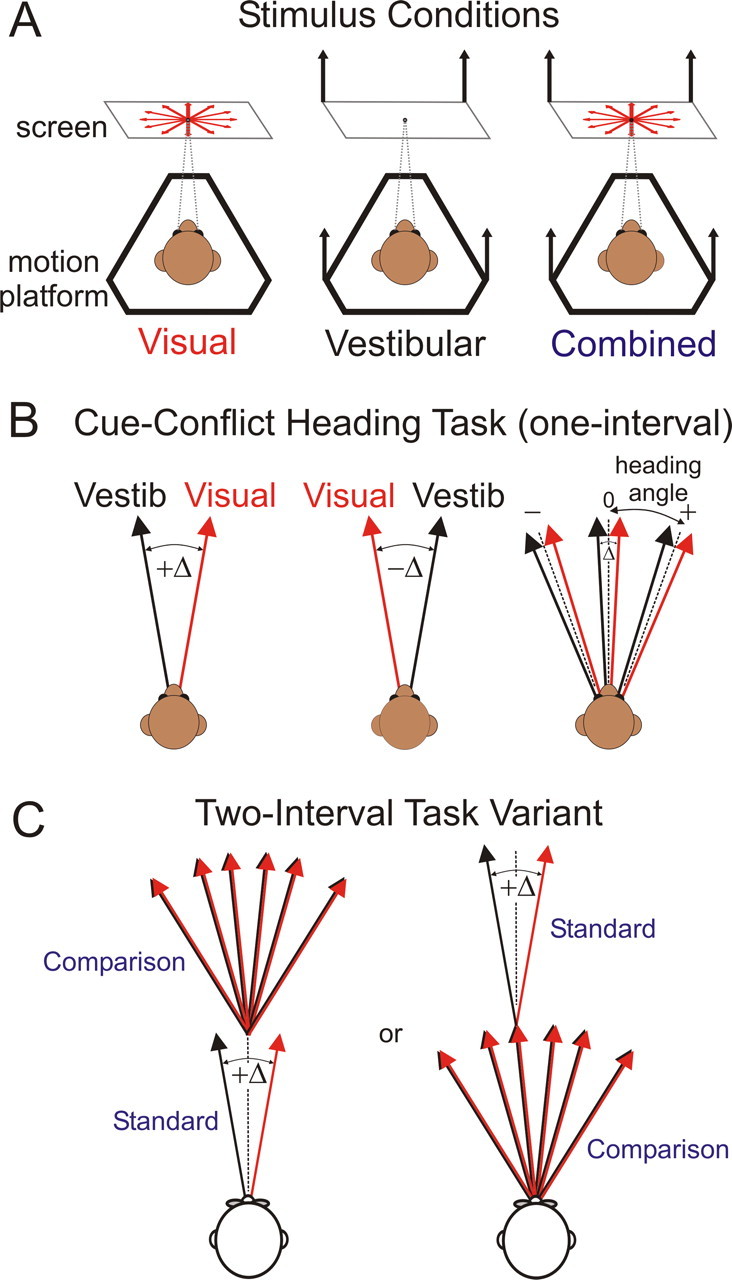
Stimuli and task. A, Top view of the three stimulus conditions used in the heading discrimination task: visual (optic flow only, indicated by the red expanding optic flow pattern), vestibular (platform motion only, indicated by the black arrows), and combined (optic flow and platform motion). In all conditions, the monkey was required to fixate a central target during the stimulus and then saccade to a rightward or leftward target at the end of each trial to indicate its perceived heading relative to straight forward (one-interval version) or relative to the first interval (two-interval version). The heading depicted in this schematic is straight forward (0°), and thus there would be no correct answer (monkey was rewarded randomly). B, Stimulus arrangement during cue-conflict trials in the one-interval version of the task (angles not to scale). Positive Δ (left) indicates visual to the right, vestibular to the left, and vice versa for negative Δ (middle). For a given Δ (right), heading angle was defined as the midpoint between the visual and vestibular heading trajectories, which were varied together in fine steps around straight forward (positive heading angle indicates rightward motion). C, Two-interval variant of the task, used in human subjects, in which the subject must judge the heading angle of the second stimulus relative to the first. The standard interval was always straight forward, except in conflict trials when the visual and vestibular heading would be displaced to the right and left of straight forward by Δ/2. The comparison heading varied in small steps around the standard and was always cue consistent. The order of presentation could be either standard first and comparison second (left) or vice versa (right).

In all stimulus conditions, the task for animal subjects was a one-interval, two-alternative forced-choice (2AFC) heading discrimination (Fig. 1 B), using the method of constant stimuli. In each trial, the monkey was presented with a (real or simulated) translational motion stimulus in the horizontal plane (Gaussian velocity profile; peak velocity, 0.45 m/s; peak acceleration, 0.98 m/s²; total displacement, 0.3 m; duration, 2 s). The heading angle was varied in small (logarithmically spaced) steps around straight ahead, and the monkey was required to indicate his perceived heading relative to straight forward by making a saccade to one of two choice targets illuminated at the end of the trial. Combined condition trials were randomly assigned one of three conflict angles: +Δ, −Δ, or 0 (no conflict). Positive Δ indicates visual to the right and vestibular to the left (vice versa for negative Δ) (Fig. 1 B), and the magnitude of Δ was 4° unless otherwise specified. When Δ was nonzero, “heading angle” was defined as the mean of the trajectories specified by visual and vestibular cues (i.e., each cue was offset from the heading angle by Δ/2 in opposite directions). Relative cue reliability was varied by manipulating the motion coherence of the optic flow pattern. For example, 25% coherence indicates that 25% of dots in a given video frame moved coherently to simulate the intended heading direction, whereas the remaining 75% of dots were randomly relocated within the three-dimensional cloud. Vestibular cue reliability was held constant.

Typically, 15–20 stimulus repetitions were presented in a block of trials (945–1260 total trials, one block per day), in which each repetition includes seven heading angles (typically 0°, ±1.23°, ±3.5°, and ±10°; positive indicates rightward, negative indicates leftward), three stimulus conditions (visual, vestibular, and combined), two coherence levels (one of the six possible pairs chosen from 12, 24, 48, and 96%), and three conflict angles (Δ = 0°, ±4°), all randomly interleaved. Two animals (monkeys A and C) were tested with two additional magnitudes of conflict angle, Δ = ±2° and ±6°, in separate blocks. At least 12 blocks (180–240 repetitions) were collected in total for each animal, including two blocks of each of the six possible coherence pairs (12–24, 12–48, 12–96, 24–48, 24–96, and 48–96) in pseudorandom order across days. For monkey I, an additional two coherence levels (8 and 16%) were tested. After all other data were collected, monkeys C and Y were tested in 10–12 additional sessions without binocular disparity cues. In these sessions, the monkeys still wore red–green glasses but viewed yellow dots such that no disparity was added and all dots appeared in the plane of the display screen.

Reward contingencies.

Human studies of this kind (Landy and Kojima, 2001; Ernst and Banks, 2002) typically do not give feedback regarding correct or incorrect choices. In contrast, monkey psychophysics generally requires frequent rewards to sustain motivation and attention to the task. In standard manner, we rewarded correct trials with a drop of water or juice; however, on some cue-conflict trials, the correct answer was undefined. This occurs when the heading angle is less than half the conflict angle (e.g., heading angles of 0° or ±1.23° when Δ = ±4°), such that the visual cue specifies a rightward heading (relative to straight forward) and the vestibular cue a leftward heading, or vice versa. On these ambiguous trials, monkeys were rewarded independently of choice, with a fixed probability chosen to match the average correct rate for the same heading angles when Δ = 0° (typically 60–65%). We also reduced the overall reward rate slightly: monkeys were rewarded on 92–95% of correct trials. This was intended to make rewards less deterministic, such that the animals would be less likely to notice the random reward contingency on ambiguous trials.

Human subjects and task.

The study was approved for human subjects by the Washington University Human Research Protection Office. Six subjects (four male) with normal or corrected-to-normal vision and no known vestibular deficits were recruited for the study and gave informed consent. Three subjects were naive to the experimental aims, and one was a coauthor (C.R.F.). Data from one of the naive subjects were discarded because of large biases resulting in unreliable threshold estimates. Subjects were seated comfortably in a cockpit-style chair, restrained with a five-point racing harness and a thermoplastic mask for head stabilization. The chair was mounted on an identical motion platform as in the monkey experiments and situated facing a large (100° × 100°) projection screen anchored to the platform. Subjects wore liquid crystal display-based active three-dimensional glasses (CrystalEyes 3; RealD) to provide stereoscopic depth cues and headphones for providing trial timing-related feedback (a tone to indicate when a trial was about to begin and another when a button press was registered). No feedback about correct or incorrect choices was provided.

The task for human subjects was a two-interval version of the 2AFC heading task (Fig. 1 C) in which each interval consisted of a 1 s motion stimulus (peak velocity, 0.27 m/s; peak acceleration, 0.9 m/s²; total displacement, 13 cm). One of the intervals was designated the “standard” and was always a straight forward movement. The other interval was the “comparison” and its heading varied in fine steps around the standard. Subjects were instructed to report (via a button press) whether their perceived self-motion direction in the second interval was to the right or left relative to the first interval. The experimenter also encouraged them to pay attention as much as possible to both cues (optic flow and inertial motion) when both were present. The cue conflict, when present, was only added to the standard interval. The temporal order of the standard and comparison was randomized across trials to prevent the subject from ignoring the standard and performing a one-interval task using only the comparison. Note that, for near-threshold heading angles, subjects were unlikely to be aware of which interval contained the standard and which contained the comparison; their task was always to compare the second interval relative to the first, and the choice data were recoded as “comparison versus standard” during offline analysis.

The task did not require extensive training, although one to four practice sessions were given to each subject before data collection. Based on these practice sessions and pilot data with other subjects, we chose a different set of four coherence levels (25, 35, 50, and 70%) designed to span the typical range of vestibular thresholds in our subjects (and thus to provide a wide range of predicted vestibular weights; see below, Data analysis). After the practice sessions, one subject (I) did not perform above chance for visual-only trials at 25% coherence, and thus a higher coherence level (90%) was added to that subject's protocol and the 25% level was removed.

At least 20 repetitions of each combination of heading angle, stimulus condition, motion coherence, and conflict angle were collected for each subject, for a total of at least 1260 trials over 3–6 weeks. A typical 1 h session included three to four repetitions (189–252 trials) of each stimulus condition at one of the six possible coherence pairs (25–35, 25–50, 25–70, 35–50, 35–70, or 50–70). Seven heading angles (0°, ±1.96°, ±5.6°, and ±16°) and five conflict angles (0°, ±2.5°, ±5°) were used, except for subject I in which the ±5° conflict was omitted. Because of technical limitations, the three stimulus conditions (visual, vestibular, and combined) were tested in separate blocks (in pseudorandom order) for a given session; however, the coherences and conflict angles were still randomly interleaved within the combined-condition block.

This two-interval task is very similar to that used in previous human psychophysical studies (Ernst and Banks, 2002; Alais and Burr, 2004) and is advantageous because it requires fewer assumptions regarding the source of variability in the estimates (i.e., in the one-interval task, the variance of the internal, remembered standard is unknown). We intended to use the two-interval task for monkeys as well but found it very difficult to train animals to make a relative heading judgment. Two of the first three animals we attempted to train on both tasks showed a strong tendency to discriminate around an internal reference of straight forward, regardless of the reference heading presented in the standard interval. Only one animal, monkey I, was able to generalize the standard to multiple eccentric heading angles, thereby demonstrating a true relative judgment. Because of this, we proceeded with the monkey experiments using only the one-interval task. There were no other major differences in the experimental design and analysis for the two task variants, and the basic trends in the data for monkey I were similar across tasks (supplemental Fig. 1, available at www.jneurosci.org as supplemental material). The main difference is that the two-interval task was more difficult for this animal (higher thresholds for a given coherence) (supplemental Fig. 1A vs B, available at www.jneurosci.org as supplemental material), which also slightly affected the weights (supplemental Fig. 1C vs D, available at www.jneurosci.org as supplemental material). However, the main result of robust cue reweighting with changes in coherence was present in both tasks.

Data analysis.

Analyses and statistical tests were performed using Matlab R2007a (MathWorks) and SPSS Statistics 17.0. For each subject, coherence level, stimulus condition, and conflict angle, separate psychometric functions were constructed by plotting the proportion of rightward choices as a function of heading angle. These data were fitted with a cumulative Gaussian function using psignifit version 2.5.6 (http://bootstrap-software.org/psignifit/), a Matlab software package that implements the maximum-likelihood method of Wichmann and Hill (2001a). The psychophysical threshold and point of subjective equality (PSE) (also known as the bias) were taken as the SD (σ) and mean (μ), respectively, of the best-fitting function. For most analyses, psychometric data were pooled across sessions before fitting; the only exceptions were the scatter plot in Figure 6 (to examine deviations from optimality in individual sessions) and the without-disparity threshold data in Figure 7, C and D (for consistency with our previous work).

Figure 6.

Correlation between optimality in weights and thresholds. For each session, deviation from the optimal (predicted) vestibular weight was plotted as a function of the ratio of actual to predicted combined thresholds, color coded by monkey identity. The left and right halves of the plot contain sessions in which the animal performed better or worse than the prediction, respectively. The upper quadrants indicate vestibular over-weighting (visual under-weighting) and vice versa for the lower quadrants. The significant correlation (r = 0.375, p < 0.0001) implies that the over-weighting of the vestibular cue goes hand in hand with the inability to show improved discrimination performance in the combined condition.

Figure 7.

Lack of an effect of binocular depth cues on weights and thresholds. Two monkeys were tested in additional sessions with stereo cues removed from the optic flow stimulus. Performance without disparity cues remained close to optimal predictions for both the weights (A) and thresholds (B–D).

From the thresholds in the single-cue (visual and vestibular) conditions, we used Equation 2 (replacing A and B with visual and vestibular) to compute the “predicted” weights for a statistically optimal observer. Note that we assume a model in which the weights sum to 1; for simplicity, we will typically report only the vestibular weight. We then compared these predicted weights with “actual” weights derived from the combined condition data, as follows (for a demonstration of the logic of this analysis using simulated data, see Fig. 2). Consider the case of positive Δ, i.e., when the visual heading is displaced to the right and the vestibular to the left by Δ/2. One can estimate the weight given to each cue by measuring the shift of the PSE (or μ) relative to the zero-conflict condition. Note that the PSE is referenced to the midpoint of the two cues (the heading angle, used as the abscissa for the psychometric functions). Thus, if the PSE is shifted to the right by Δ/2 (Fig. 2, black dot and dashed lines), it means that the subject chose rightward 50% of the time when the vestibular motion trajectory was aligned with straight forward and the visually defined trajectory was rightward. The only way this could occur is if the subject's heading estimate was derived 100% from the vestibular cue and 0% from the visual cue; hence, the vestibular weight in this case would be 1 (“vestibular capture”; also notice that, at heading angle 0, at which the vestibular cue signals leftward and the visual cue rightward, the proportion of rightward choices for this curve is near 0%). If instead the PSE is shifted to the left by Δ/2 (Fig. 2, red dot and dashed lines), it means the subject is using only the visual cue, i.e., a vestibular weight of 0 (“visual capture”). No shift of the PSE (cyan) indicates equal weights of 0.5 for the two cues.

Figure 2.

Simulated data demonstrating the method for measuring actual cue weights. For simplicity, this example considers only the case of +Δ (visual to the right, vestibular to the left) in the one-interval version of the task. The leftmost psychometric curve would be observed if the subject were completely ignoring the vestibular cue (visual capture, or a vestibular weight of 0). This can be understood by thinking of the PSE (red dot) as the heading angle at which the subject “feels” that his motion was straight forward (and thus would make 50% rightward and 50% leftward decisions, assuming no choice bias). By definition, the heading angle at which this occurs is −Δ/2, and thus a (bias-adjusted) PSE of −Δ/2 maps onto a vestibular weight of 0 when Δ is positive, consistent with Equation 3. The opposite is true for the rightmost curve: the PSE (black dot) is +Δ/2, meaning that the ambiguous stimulus (perceived as straight forward) is the one in which the vestibular cue is pointing straight forward, corresponding to a vestibular weight of 1. If the PSE is 0 (cyan), it means the cues are weighted equally (weights equivalent to 0.5) and the subject estimated the heading angle to be the average of the two cues. Any PSE shift between −Δ/2 and +Δ/2 results in a vestibular weight that is scaled linearly between 0 and 1 (see axis below the abscissa). The analysis is identical for the two-interval task, except that the abscissa represents the comparison heading, and the direction of the expected PSE shift is reversed for a given weight (because the conflict is in the standard interval).

Corresponding to the analysis described above, the actual weights were computed by taking the PSEs from the +Δ and −Δ psychometric functions, adding Δ/2, and dividing by Δ [after adjusting for any overall bias by subtracting the PSE in the Δ = 0° case (μ₀)]:

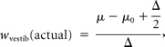Thus, maintaining the sign of Δ as defined in Figure 1 B, a rightward (positive) PSE shift when Δ is positive corresponds to a high vestibular weight, as does a leftward shift when Δ is negative (and vice versa for visual weight). Weights were computed separately for −Δ and +Δ curves and then averaged for a given coherence level. This approach is equivalent to taking the slope of the linear regression of PSE versus Δ (Ernst and Banks, 2002; Alais and Burr, 2004) and then adding 0.5 to get the vestibular weight.

For visualization purposes, the predicted weights and thresholds were converted into predicted psychometric functions using the Matlab function normcdf, in which the mean (μ) was computed from Equation 3 (replacing the left side of the equation with the predicted weight and then solving for μ) and the SD (σ) was computed from Equation 1. These are illustrated as dashed curves in Figure 3 B–E.

Figure 3.

Example psychometric functions. The proportion of rightward decisions is plotted against heading angle, including all data from a single animal (monkey Y). Solid curves depict the best-fitting cumulative Gaussian function. For the single-cue conditions (A), separate curves are plotted for the vestibular condition (black circles) and visual condition at each of the four coherence levels tested (12, 24, 48, and 96%, coded as different shapes and progressively darker shades of red). For the combined condition data, separate plots (B–E) are made for each coherence level, and within each plot the data are separated by conflict angle [blue, Δ = −4° (visual to the left of vestibular); cyan, Δ = 0° (cue consistent); green, Δ = +4° (visual to the right of vestibular)]. Dashed curves represent the predicted psychometric functions for each Δ, based on the predicted cue weights computed from single-cue thresholds (Eq. 2). These dashed curves were given the predicted thresholds derived from Equation 1 and were offset to match the overall bias (represented by the cyan solid curve), consistent with the manner in which we computed actual cue weights (see Eq. 3 and associated text). The reversal of the green and blue curves from low (B, C) to high (D, E) coherence indicates a shift from vestibular dominance to visual dominance (for additional explanation, see Fig. 2 and Materials and Methods).

Behavioral simulation.

To evaluate possible effects of the variable reward schedule and non-uniform stimulus prior (see Results), we conducted a simple simulation of the monkeys' performance in the heading discrimination task. On a given trial of the simulation, a heading stimulus was drawn from the same set of stimulus conditions, heading angles, conflict angles, and coherence levels used in the experiments. The model then computed likelihood functions representing the noisy sensory evidence (from visual and/or vestibular cues) on that trial. Incorporating biologically plausible assumptions about noise in sensory coding, these likelihood functions were not forced to align with the true stimulus value on a given trial but rather were computed from the population response of N simulated Poisson neurons (see below). The tuning functions of these neurons were linear over the range of heading angles tested (−10° to 10°) and varied in slope from −sm to +sm, in which m is a constant and s is a scaling factor related to the reliability of the sensory evidence (i.e., motion coherence). Our choices for the tuning shape and effect of coherence are broadly consistent with physiological results from the dorsal medial superior temporal area (MSTd) (Gu et al., 2008), a region implicated in visual–vestibular integration for heading perception. However, the main conclusions from the simulation were not dependent on linear tuning or particular values for the free parameters N, m, and s. Because our goal was simply to rule out uncontrolled effects of the reward schedule and a hypothetical stimulus prior (not to fit a comprehensive model to the behavioral data), we manually chose the values of these parameters to be N = 40, m = 0.25 spikes/s/°, and s = [1, 2, 3, 4] for coherence = [12, 24, 48, 96]. The scaling factor s was set to 2 when simulating the vestibular cue. With these values, the model produced discrimination thresholds similar to what we observed in our monkey experiments.

The response of each model neuron on a given trial was drawn from a Poisson distribution with mean and variance equal to the value of the tuning function of that neuron at the simulated heading angle. The population response of the 40 model neurons was then used to compute the likelihood function using well known analytical methods (Foldiak, 1993; Seung and Sompolinsky, 1993; Sanger, 1996; Dayan and Abbott, 2001; Jazayeri and Movshon, 2006; Ma et al., 2006), in this case via an expression derived from the probability mass function of an independent Poisson random variable:

Here, R is the population response on a single trial on which stimulus θ was presented, f_i is the tuning function of the ith neuron in the population [i.e., f_i(θ) is the mean response of neuron i to stimulus θ], and r_i is the response of neuron i on that particular trial. Note that this formulation treats p(R|θ), sometimes written L_R(θ), as a function of θ and thus describes the relative likelihood of every possible θ given the response pattern R. As shown in supplemental Figure 3 (available at www.jneurosci.org as supplemental material), the likelihood function for each simulated trial at a particular heading is a bell-shaped function. In the absence of neuronal noise, the likelihood function would peak at the same heading (the true value) on every trial. However, Poisson noise causes the simulated likelihood to shift around from trial to trial, and this ultimately gives rise to the stochastic choices made by the simulated observer. At low coherence, the likelihood function for visual stimuli is broader and shifts more from trial to trial than at high coherence (supplemental Fig. 3, available at www.jneurosci.org as supplemental material), thus leading simulated performance to depend on coherence.

In each simulated trial, the posterior distribution was computed as the product of the likelihood(s) and the prior, which was modeled as an exponential distribution λe ^−λx (mirrored across 0 for negative heading values). The rate parameter λ was manually set to 0.16, with the goal of having each multiplicative step on the x-axis (i.e., expanding bins centered on the experimental heading angles) cover a region of approximately equal area. The logarithmically spaced headings used in the task can be considered a discrete approximation to this broad exponential prior (supplemental Fig. 5A, available at www.jneurosci.org as supplemental material). However, the choice of a particular shape for the prior did not greatly affect the outcome of the simulations, provided it was symmetric around 0° and broad enough to include the largest heading angles used in the experiments (±10°) with some reasonable probability. Similar results were obtained with other formulations of the prior (e.g., Gaussian).

The simulation used a simple maximum a posteriori decision rule, taking the sign of heading at the peak of the posterior distribution as its choice on each trial (positive indicates right, negative indicates left). Twenty repetitions of each stimulus condition were run for a given iteration of the model, and cumulative Gaussian functions were fit to the choice data (proportion of rightward decisions vs heading angle) as described above. In the same manner as the real experimental data, the fitted psychometric functions from the simulated single-cue and combined conditions were used to compute predicted and actual weights, respectively.

To simulate different choice strategies on the ambiguous (randomly rewarded) trials, the choice dictated by the posterior on these trials was overridden by either a random-choice (coin flip) or a fixed-choice (right or left) bias on a specified proportion of trials, denoted P _random (see Results) (supplemental Fig. 4, available at www.jneurosci.org as supplemental material). We varied P _random across each set of model iterations to systematically characterize the effect of random or biased choices on cue weights. Each trace in supplemental Figure 4 (available at www.jneurosci.org as supplemental material) represents the average ± SEM weights from a set of 20 iterations.

Results

We collected behavioral data from five rhesus monkeys and five human subjects performing a heading discrimination task (Gu et al., 2007, 2008) using optic flow (visual condition), inertial motion (vestibular condition), or a combination of both cues (combined condition) (Fig. 1 A). On two-thirds of combined trials, a small conflict angle (Δ) was interposed between the visual and vestibular heading trajectories (Fig. 1 B). Cue reliability was varied randomly across trials by changing the motion coherence of the optic flow stimulus.

Reliability-based cue reweighting in monkeys

Single-cue behavior for one animal (monkey Y, pooled across sessions) is shown in Figure 3 A. These psychometric functions illustrate the proportion of rightward choices as a function of heading angle (negative indicates leftward, positive indicates rightward). The varying reliability across single-cue conditions is evident from the different slopes of the psychometric functions, which we quantify by taking the SD (σ, also called the threshold) of the best-fitting cumulative Gaussian function. Note that the four coherence levels were chosen such that the visual thresholds spanned a large range, including values smaller and larger than the vestibular threshold. The average vestibular threshold for this animal (black circles and curve) was 2.8°, and the visual thresholds for the four levels of motion coherence (12, 24, 48, and 96%) were 7.3°, 2.8°, 1.8°, and 1.0°, respectively (light pink to dark red curves). From these single-cue thresholds, we computed the weights that the monkey should use if he were to optimally combine the two cues (Eq. 2). Each coherence level has a different predicted weight, computed from each pairing of the fixed vestibular threshold with the varying visual thresholds. The predicted vestibular weights for this animal were 0.85, 0.53, 0.28, and 0.12, ranging from vestibular dominance to visual dominance as coherence is increased.

Figure 3 B–E shows the actual combined condition results (circles and solid curves) for the same animal. The four coherence levels are illustrated in separate panels, each with three psychometric functions representing the three conflict conditions (for definitions, refer to Fig. 1 B): Δ = −4° (blue), Δ = 0° (cyan), and Δ = +4° (green). When visual cue reliability was low (12% coherence) (Fig. 3 B), the psychometric functions during cue conflict shifted in the direction that indicates vestibular dominance (blue curve to the left, green curve to the right). This shift was well predicted by the optimal cue integration model, as shown by the dashed curves, which are derived from the single-cue data (for details, see Materials and Methods). In contrast, when visual reliability was high (96% coherence) (Fig. 3 E), the curves shifted in the opposite directions, indicating visual dominance. The optimal predictions for all four coherence levels, shown by the dashed curves, reproduce the trends in the actual data (solid curves) quite well. As described in Materials and Methods, the monkey's actual cue weights were computed from the measured shifts of the psychometric functions. For this animal, the actual vestibular weights for the four coherence levels were 0.87, 0.67, 0.31, and 0.0, respectively, compared with predicted weights of 0.85, 0.53, 0.28, and 0.12. Importantly, this cue reweighting must occur dynamically, from trial to trial, as coherence was varied at random within each block of trials.

Predicted and actual weights [±95% confidence intervals (CIs)] are summarized for the five monkeys separately in Figure 4 A–E and averaged across monkeys in Figure 4 F. The main result is that all animals show robust changes in actual weights, moving from high to low vestibular weight (low to high visual weight) as coherence increases (Spearman's rank correlation: r < −0.86, p < 0.0001). Some animals' weights align quite well with the predictions [monkeys Y and I (Fig. 4 A,B)], whereas others clearly do not [monkey A (Fig. 4 E)]. On average, monkeys tend to modestly over-weight the vestibular cue (or under-weight the visual cue) in this task (Fig. 4 F) compared with the optimal predictions derived from single-cue thresholds (Eq. 2). To test for a significant difference between predicted and actual weights while controlling for the large effect of coherence, we used a general linear model that is best described as a repeated-measures analysis of covariance (rm-ANCOVA). In this model, the weights are the dependent variable (with predicted vs actual being the paired or repeated measure), motion coherence is the covariate (continuous predictor), and monkey identity is a categorical factor. This analysis revealed a significant main effect of predicted versus actual weights (F = 18.6, df = 1, p < 0.001) and a significant interaction between predicted versus actual weights and monkey identity (F = 8.4, df = 4, p = 0.001), as well as confirming the strong overall effect of coherence (F = 48.4, df = 1, p < 0.0001). We consider possible reasons for the over-weighting of vestibular cues during heading perception in Discussion.

Figure 4.

Summary of predicted and actual cue weights. Vestibular weight (1 − visual weight) is plotted as a function of visual motion coherence for each of five monkey subjects (A–E) and averaged across subjects (F). Predicted weights (open symbols) were computed from Equation 2 using single-cue thresholds, and actual weights (filled symbols) were computed from the shift of the PSE relative to the magnitude of cue conflict (see Eq. 3 and Fig. 2). Error bars in A–E represent 95% CIs computed using the following bootstrap procedure. Choice data were resampled across repetitions (with replacement) and refit 250 times to create distributions of the PSE and threshold for each psychometric function. We then drew 1000 random samples from these distributions to compute 1000 bootstraps of predicted and actual weight (Eqs. 2, 3) and computed the CIs directly from these bootstraps (percentile method). Similar CIs were obtained using error propagation (data not shown). Error bars in F represent ±SEM across subjects.

For two animals (C and A), we also varied the magnitude of the conflict angle (Δ = ±2°, 4°, and 6°) (supplemental Fig. 2, available at www.jneurosci.org as supplemental material). The effects of conflict magnitude (|Δ|) were mixed and differed between the two animals. For monkey C, conflict magnitude had little effect, whereas it had a clear effect for monkey A. Adding |Δ| as a factor in the rm-ANCOVA showed a significant interaction effect (predicted vs actual * |Δ|; F = 4.7, df = 2, p = 0.02) but no main (between-subjects) effect of |Δ| (F = 0.05, df = 2, p = 0.96). The interaction effect was driven mainly by monkey A, whose actual vestibular weights were substantially lower (and closer to the prediction) when conflict angle was ±6°. A similar examination of conflict magnitude in the human experiments yielded no significant effect of |Δ| on the weights, as discussed below (see Fig. 7). Most importantly, the essential result of Figure 4 (and supplemental Fig. 2, available at www.jneurosci.org as supplemental material) is that perceptual weights depend strongly on coherence for all animals and for all values of |Δ|.

Combined thresholds and the relationship between weights and thresholds

As mentioned above, optimal cue integration models also predict an improvement in threshold when both cues are present (Eq. 1). Although this prediction was tested previously using a single coherence level (Gu et al., 2008), the larger dataset in the present study gives us an opportunity to examine the threshold prediction in more animals and across multiple coherence levels (monkey C was also used in that previous study). Figure 5 plots the single-cue (red squares, visual; black squares, vestibular), predicted (open blue circles), and actual (filled blue circles) combined thresholds separately for each animal (A–E) and averaged across animals (F). Both visual (Spearman's r = −0.86, p < 0.0001; computed from the psychometric fits of pooled data, i.e., one data point per monkey per coherence) and combined thresholds (r = −0.64, p = 0.003) clearly decrease as a function of coherence. Vestibular thresholds, by definition, do not vary with coherence but are the same data replotted at each point for comparison. On average, the actual combined thresholds (Fig. 5 F, filled blue circles) were similar to, but significantly greater than, the predicted thresholds (open blue circles). We again used an rm-ANCOVA model to test the hypothesis that predicted versus actual combined thresholds differed, while controlling for effects of coherence and monkey identity. This model yielded significant main effects of predicted versus actual threshold (F = 7.4, df = 1, p = 0.02), monkey identity (F = 3.9, df = 4, p = 0.03), and their interaction (F = 7.1, df = 4, p = 0.002).

Figure 5.

Summary of psychophysical thresholds. For each monkey, single-cue visual (red squares) and vestibular (black squares) discrimination thresholds are plotted against coherence, along with the predicted (blue open circles) and actual (blue filled circles) combined thresholds. Error bars for actual thresholds (single-cue and combined) represent 95% CIs from the psychometric fits themselves (Wichmann and Hill, 2001b), whereas for predicted combined thresholds, they represent bootstrapped CIs via the method described in the legend of Figure 4, except using Equation 1 instead of Equations 2 and 3.

This significant interaction with monkey identity highlights the clear variation in performance across animals. For example, combined thresholds for monkeys Y and C are well matched to predicted thresholds, whereas for monkey A they are not (and in fact are worse than the best single-cue threshold in most cases). Notably, the weights for monkey A (Fig. 4 E) were also the most discrepant from the optimal prediction. From the standpoint of the Bayesian framework, deviations from optimality in the weights would be expected to correlate with deviations from optimality in the thresholds, because both predictions (Eqs. 1, 2) are derived from the same formulation in which the distribution of the combined estimate is given by a product of the single-cue likelihoods. To examine this relationship in more detail, we plotted the deviation from optimality in weights [the difference w _ves(actual) − w _ves(predicted)] versus the deviation from optimality in thresholds [the ratio σ_comb(actual)/σ_comb(predicted)]. For this analysis, we used psychometric data from individual sessions (one data point per session) rather than pooling across sessions. The result is shown in Figure 6, color coded by monkey and including data from all coherence levels. The overall correlation is significant (Spearman's r = 0.375, p < 0.0001), and monkey A (blue circles) can be seen as a distinct cluster primarily in the upper right quadrant. Data from monkey Y (red), conversely, cluster closer to the optimum for both weights and thresholds (intersection of the dashed lines).

We note that a linear relationship between these two variables (i.e., correlation) would not be expected if visual over-weighting occurred approximately as often as vestibular over-weighting. In that case, the plot would show a rightward facing v-shape, because visual over-weighting (points below the horizontal dashed line) would also be expected to inflate combined thresholds above the prediction. Nevertheless, the observed correlation between vestibular over-weighting and increased thresholds suggests that both may arise from suboptimal performance of a mechanism that attempts to weight cues according to their reliability (for example, by computing a product of likelihood functions).

Lack of an effect of binocular disparity cues

One consideration in designing our optic flow stimuli was that an absolute depth cue might be important for enabling the integration of visual motion with inertial motion cues (Martin S. Banks, personal communication). Without depth information or a reference object of known size, the scale of the virtual space, and thus the speed and distance of simulated motion, is ambiguous (the “scaling problem” of optic flow). Hypothetically, scale-ambiguous optic flow might not be interpreted by the brain as a consistent, plausible self-motion cue when presented along with inertial motion. Indeed, anecdotal observations during training of our first animal suggested that binocular disparity cues were required for the monkey to exhibit improvement in combined thresholds relative to the single-cue conditions (Y. Gu, G. C. De Angelis, and D. E. Angelaki, unpublished observations). Preliminary evidence in human subjects (J. S. Butler, H. H. Bülthoff, and S. T. Smith, unpublished observations) also supports this conclusion. As a result, disparity was included in the stimuli for subsequent experiments.

Once several animals were trained in the task, we returned to the question of disparity cues, repeating the full cue-conflict paradigm in monkey C without stereo. Surprisingly, there was no significant effect of removing stereo cues on either the weights (rm-ANCOVA, p = 0.38) (Fig. 7 A) or thresholds (p = 0.2) (Fig. 7 B). We also repeated the behavioral paradigm of Gu et al. (2008) in monkey Y in the absence of disparity cues. This paradigm uses a single coherence level that provides the best match between single-cue visual and vestibular thresholds, to maximize the ability to observe an improved combined threshold (Eq. 1). Figure 7 C plots the mean ± SEM (across individual sessions) single-cue and combined threshold data for this experiment (without disparity), showing a combined threshold significantly lower than the single-cue thresholds and not significantly different from the prediction (paired t tests) (Fig. 7 C). For comparison, we replotted a portion of monkey C's no-disparity data (specifically, those sessions in which visual and vestibular single-cue thresholds were fairly well matched) in the same format in Figure 7 D. The pattern of results is similar for the two animals. These findings suggest that, although disparity information may be useful for establishing the threshold effect during initial training, it is not required for optimal visual–vestibular integration in well trained animals. Additional longitudinal experiments are necessary to confirm this interpretation.

Possible effects of reward schedule and stimulus prior distribution

Monkeys were rewarded for correct choices, but on some cue-conflict trials, the correct choice was necessarily ambiguous (see Materials and Methods). In particular, when the heading angle was ±1.23° or 0°, and Δ = ±4° (Fig. 3 B–E, available at www.jneurosci.org as supplemental material), the visual and vestibular heading angles straddled straight forward, and thus each cue dictated a different response. In these trials, we rewarded monkeys independently of choice, to avoid biasing them toward one cue or the other. In principle, this stochastic reward schedule could have affected the monkeys' choices on ambiguous trials; for example, if they were able to detect that rewards were not contingent on their decisions, they could have chosen left or right without regard to the stimulus and still maintained the same total reward rate. That this did not occur is evident in the raw data (Fig. 3 B–E): if decisions during ambiguous trials were random, the three central blue and green data points would align horizontally near the midpoint of the ordinate (50% rightward decisions). Alternatively, if monkeys had a fixed choice bias (left or right) during ambiguous trials, these points would lie near the bottom or top of the plot, respectively. More generally, these three data points are critical to the measurement of actual weights, because they primarily determine the PSE of the psychometric functions. The lack of a discontinuity in these functions, along with the goodness of fit of the cumulative Gaussian function over the range −1.23 to +1.23, suggests that this animal's behavioral strategy did not differ substantially during ambiguous trials. This is likely a consequence of using small conflict angles that were difficult to detect and the fact that ambiguous trials were a small fraction of the total (19%, randomly interleaved).

To further assess the possible consequences of our reward delivery scheme, we performed a simple simulation of behavioral performance to explore how different choice strategies might affect the measured weights (see Materials and Methods) (supplemental Fig. 4, available at www.jneurosci.org as supplemental material). As expected from the above logic, this simulation revealed that a strategy of making random choices on some proportion of the ambiguous trials served to reduce the magnitude of the PSE shift, pushing actual weights toward 0.5. This resulted in apparent vestibular under-weighting at the lowest coherence and over-weighting at the highest coherences (i.e., a flatter trace of actual vestibular weight as a function of coherence) (supplemental Fig. 4, available at www.jneurosci.org as supplemental material), with larger effects as the proportion of ambiguous trials with a random response (P _random) was increased. A similar pattern of results occurred for the strategy of a fixed left or right choice bias on ambiguous trials (data not shown). In the real data, we observed fairly consistent vestibular over-weighting, with no reversal as a function of coherence (Fig. 4). In fact, in the real data, there was little or no vestibular over-weighting at the highest coherence level, contrary to the simulation. Thus, we conclude that the pattern of results we observed was not strongly influenced by the random reward schedule on ambiguous trials.

Another potential concern is the effect of a non-uniform prior distribution of stimulus heading values. The basic theoretical predictions described by Equations 1 and 2 assume a prior over heading that is uniform or at least very broad relative to the sensory likelihood functions (Jacobs, 1999; Ernst and Banks, 2002; Knill and Saunders, 2003; Hillis et al., 2004). During the experiments, however, monkeys were exposed to a particular distribution of logarithmically spaced headings, such that heading values clustered around straight forward. If this stimulus distribution introduced a prior expectation for central headings, could this have affected monkeys' choices and hence the psychometric functions we measured?

To examine this question, the simulation included a prior that approximated the distribution of heading angles used in the experiments (see Materials and Methods). For a given configuration of cues (e.g., heading angle of +1.23° and Δ = +4°) (supplemental Fig. 5A, available at www.jneurosci.org as supplemental material), this prior had the effect of shifting the posterior slightly toward 0° and thus closer to one of the two cues (in this case, vestibular). Critically, however, the prior could never shift the peak of the posterior far enough to change the binary decision of the subject, because the prior is symmetric around 0. Rather, variation in choice across trials for the same stimulus results from random variations in the sensory likelihoods as a result of Poisson noise on the model neurons (supplemental Fig. 3, available at www.jneurosci.org as supplemental material). The product of the visual and vestibular likelihoods determined whether the choice was rightward or leftward in the simulations, and the prior just shifted the pre-decision estimate slightly toward 0. Thus, a symmetric prior cannot change the choice behavior of a Bayesian observer in a 2AFC task like ours. This lack of an effect of the prior is illustrated in supplemental Figure 5B (available at www.jneurosci.org as supplemental material), showing nearly identical psychometric functions regardless of whether the prior was included in the simulation (solid curves) or not (dashed curves).

Visual–vestibular cue integration in humans

Unlike visual–auditory (Battaglia et al., 2003; Alais and Burr, 2004; Shams et al., 2005), visual–haptic (Ernst and Banks, 2002), and visual–proprioceptive (van Beers et al., 1999) cue integration, visual–vestibular integration in humans has received less attention in the literature (but see MacNeilage et al., 2007) (see also J. S. Butler, J. L. Campos, H. H. Bülthoff, and S. T. Smith, unpublished observations). In addition to being of interest on its own, a comparison of human and monkey behavior is important to rule out species differences or effects of overtraining. Thus, we repeated the same basic design in five human subjects using an identical motion platform adapted for human use. Other than using a two-interval variant of the task (Fig. 1 C), the apparatus, stimuli, and analyses were essentially the same as those used in monkeys (see Materials and Methods).

Figure 8 summarizes the weights (A) and thresholds (B) averaged across five subjects (±SEM) and for two conflict magnitudes (|Δ| = 2.5°, 5°). Similar to monkeys, actual vestibular weights were strongly anticorrelated with coherence (r = −0.87, p < 0.0001) and were marginally significantly greater than the predicted weights (rm-ANCOVA, main effect of predicted vs actual weight: F = 5.7, df = 1, p = 0.02). There was no effect of conflict magnitude on the weights (p > 0.8 for both the main effect of |Δ| and the interaction |Δ| * predicted vs actual).

Figure 8.

Weights and thresholds for human subjects. The weights (A) and thresholds (B) are plotted in the same format as Figures 4 and 5, respectively, averaged across five human subjects (error bars represent ±SEM). Individual subject data are shown in supplemental Figure 6 (available at www.jneurosci.org as supplemental material).

The ANCOVA model also showed a significant difference between predicted and actual combined thresholds (F = 8.5, df = 1, p = 0.01), although this difference was driven primarily by a single coherence level (the upward deviation in actual thresholds at 70% coherence) (Fig. 8 B). At 35% coherence, for which there was a close match between visual and vestibular single-cue thresholds, combined thresholds were significantly lower than either single cue (paired t test, p < 0.05 for both) and not significantly different from the optimal prediction (p = 0.63), replicating our previous findings in monkeys for matched single-cue thresholds (Fig. 7 C,D) (Gu et al., 2008). Human subjects also showed some individual differences in both their weights and thresholds (supplemental Fig. 6, available at www.jneurosci.org as supplemental material), but the correlation between their respective measures of optimality [w _ves(actual) − w _ves(predicted) vs σ_comb(actual)/σ_comb(predicted)] was not significant (Spearman's r = 0.07, p = 0.68) (data not shown).

Discussion

We have developed an experimental paradigm in monkeys for studying cue integration behavior using the same type of quantitative psychophysical approach that has been successful in human studies. We found that monkeys, like humans, dynamically reweight visual and vestibular heading cues in proportion to their reliability. However, subjects placed slightly greater weight on the vestibular cue than predicted from their performance in the single-cue conditions. Nevertheless, the observation of dynamic, reliability-based cue reweighting in nonhuman primates should enable a direct investigation of the neural mechanisms that underlie this hallmark of Bayesian inference.

Previous studies of multisensory integration in animals

Visual–auditory localization in the cat, studied extensively by Stein and colleagues (Stein and Meredith, 1993; Stein and Stanford, 2008), is considered the classic animal model for behavioral and neurophysiological studies of multisensory integration. A key behavioral finding from this line of research is known as the “spatial principle”: presenting visual and auditory targets in the same location leads to improved performance compared with visual targets alone, whereas presenting the auditory target in a different location impairs performance (Stein et al., 1988, 1989; Jiang et al., 2002). These results are difficult to compare with predictions of optimal cue integration schemes (Eqs. 1, 2), because these studies were not designed for that purpose. Unlike in fine discrimination tasks (Ernst and Banks, 2002; Alais and Burr, 2004; Gu et al., 2008), performance in the discrete-target localization task used by Stein and colleagues was reported as a percentage of correct trials, with no quantification of the underlying variance of perceptual estimates (e.g., the spatial distribution of errors), as required to test probabilistic cue integration models. In fact, most “error” trials consisted of the animals failing to purposefully approach the apparatus, suggesting that they were not engaged in a localization task on those trials (i.e., were inattentive or simply failed to detect the stimuli) (Stein et al., 1989). Disrupted spatial attention, rather than bimodal integration, may also explain the impaired performance in spatially disparate trials, because the auditory cue was displaced a full 60° away from the visual target (Stein et al., 1989).

A recent study by the same group (Rowland et al., 2007) used Bayesian principles to explain the paradoxical improvement in visual localization performance when the auditory cue is more eccentric than the visual cue (a violation of the spatial principle). However, in these experiments, animals were trained to orient only to visual targets (ignoring the auditory cue), whereas the testing procedure involved near-threshold visual targets presented with suprathreshold auditory targets. Because auditory-only performance was not measured, this again leaves open the question of whether cue integration was actually taking place behaviorally (Jiang et al., 2002; Rowland et al., 2007). More importantly, the ability of their model to explain behavioral data depended on two untested assumptions (implemented by parameter fitting): (1) auditory cue reliability that decreases linearly as a function of eccentricity, and (2) a prior distribution that favored centrally located stimuli. Because these assumptions were not empirically verified with behavioral measurements, it remains unclear whether visual–auditory cue integration in the cat is statistically optimal. In contrast, we have explicitly measured vestibular and visual cue reliability to generate predictions from an optimal integration model (with no free parameters) and then tested these predictions during combined trials with small cue conflicts.

Behavioral evidence for visual–vestibular interactions in self-motion perception

The interplay of visual and vestibular signals was first studied in the context of vection, the illusory sensation of self-motion induced by visual motion (Mach, 1875; Brandt et al., 1972; Berthoz et al., 1975; Dichgans and Brandt, 1978; Howard, 1982). Subsequent work addressed the contributions of visual and vestibular cues to perception of self-motion direction (Telford et al., 1995; Ohmi, 1996) and distance (Harris et al., 2000; Bertin and Berthoz, 2004). These studies showed that human subjects could, in some conditions, achieve greater precision in estimating self-motion when both cues were provided. However, a comprehensive, mechanistic explanation of these phenomena has remained elusive, perhaps in part because they were not studied within a theoretical framework that takes into consideration cue reliability. The Bayesian framework was first applied to integration of visual and vestibular cues in our previous work (Gu et al., 2008), in which monkeys were trained to perform a multimodal heading discrimination task. In that study, visual and vestibular cue reliability was carefully matched to maximize the predicted decrease in thresholds during combined stimulation (Eq. 1), and results closely followed the prediction from Equation 1 (Gu et al., 2008). Importantly, that study could not address the second major prediction of optimal cue integration theory—dynamic reweighting of cues in proportion to their reliability (Eq. 2)—which has now been established in the present work.

Why do subjects over-weight vestibular cues?

Ours is not the first study to find deviations from optimality in cue weights. The size of the deviation we found is similar to that reported by Knill and Saunders (2003) for visual slant estimation, although in their case it was not statistically significant. Other studies (Battaglia et al., 2003; Oruç et al., 2003; Rosas et al., 2005) have found suboptimal behavior or have been forced to modify the standard Bayesian model to explain their results. Battaglia et al. (2003) found that subjects over-weighted visual cues in a visual–auditory localization task. They accounted for this effect by adding a type of prior that scaled down the variance of their subjects' visual estimates, thereby scaling up the predicted visual weights to better match to the actual weights measured in the auditory–visual condition. The authors acknowledged that this approach is akin to curve-fitting and does not provide additional explanatory power on its own. A similar modification of the model would provide a better fit to our data as well, but this was not the goal of our study.

Another possible source of the vestibular “bias” we observed in monkeys is their training history. Monkeys were initially trained to report their self-motion direction in the vestibular condition only. Once they performed reasonably well, the combined condition was introduced and coherence gradually increased from 0. Only then did the visual condition follow. The logic was to associate noisy optic flow with self-motion, to discourage the monkeys from using local motion discrimination strategies in the visual condition. This training approach might have led to vestibular over-weighting in our monkeys, although two lines of evidence argue against this conclusion. First, not all monkeys over-weighted the vestibular cue (Fig. 4), despite sharing the same training history. Second, the vestibular bias was also observed in human subjects that did not undergo this same training regimen. Human subjects were instructed to report their “self-motion direction” in all conditions, and it was made clear to them that optic flow was intended to simulate self-motion. A similar result in humans and monkeys despite different training history argues against this explanation for the vestibular bias.

A different class of explanation involves causal inference models (Körding et al., 2007; Sato et al., 2007) in which multisensory perception proceeds in two steps: (1) determining the information provided by each cue (the sensory likelihoods) and (2) assessing the probability that the two cues arose from a single source versus multiple sources (for similar ideas, see Roach et al., 2006; Cheng et al., 2007; Knill, 2007). In the case of heading estimation, causal inference might be invoked to resolve whether optic flow indicated self-motion or was instead caused by motion in the environment. Arguably, there was no such ambiguity to resolve regarding the source of vestibular cues. An imbalance in the certainty of causation between visual and vestibular cues might have produced the vestibular over-weighting we observed. To test this speculation, future experiments could ask subjects to report their perceived heading from each cue separately, even when both are presented together (a dual-report paradigm) (Shams et al., 2005) or could ask subjects to indicate in each trial whether they perceived a conflict between the cues (Wallace et al., 2004).

If causal inference was involved, subjects should infer multiple sources more often as conflict magnitude increases (Körding et al., 2007). However, we did not observe greater deviations from optimality (e.g., a larger vestibular bias) when conflict angle was increased to 5 or 6° (Fig. 8 A) (supplemental Fig. 2, available at www.jneurosci.org as supplemental material), even though this was well above the smallest single-cue threshold. It might be the case that larger conflict angles are necessary to probe causal aspects of multisensory integration in our task.

Candidate neuronal substrates for visual–vestibular cue integration

Unlike visual–auditory integration (Stein, 1998; Wallace et al., 1998), the neural basis of visual–vestibular integration remains poorly understood. Areas traditionally recognized as “vestibular cortex” (Schwarz and Fredrickson, 1971; Grüsser et al., 1990; Fukushima, 1997) appear to be primarily unresponsive to optic flow (A. Chen, D. E. Angelaki, and G. C. DeAngelis, unpublished observations) and thus seem unlikely to subserve visual–vestibular integration for heading perception. Instead, recent work points toward areas such as the MSTd (Tanaka et al., 1986; Tanaka and Saito, 1989; Duffy and Wurtz, 1991, 1995; Britten and van Wezel, 1998; Duffy, 1998) and ventral intraparietal area (Schaafsma and Duysens, 1996; Bremmer et al., 2002a,b). Gu et al. (2008) found that MSTd neurons with congruent visual and vestibular tuning showed increased heading sensitivity when both cues were presented together. The average improvement was close to the optimal prediction, suggesting that signals in MSTd may contribute to the behavioral improvement in this task.

It remains to be seen whether and how MSTd neurons dynamically reweight cues according to their reliability. Our previous work (Morgan et al., 2008) suggested that MSTd neurons compute weighted sums of their inputs, in which the weights vary with cue reliability (motion coherence). However, in that study, coherence was held constant across trials within a block, and the monkey was not using the stimuli to perform a perceptual task. In the context of perceptual discrimination, recent computational models (Pouget et al., 2003; Deneve and Pouget, 2004; Jazayeri and Movshon, 2006; Ma et al., 2006) have described how neural populations might combine probability distributions to perform optimal cue integration, but neurophysiological studies testing their predictions are scarce. The behavioral paradigm described here should be useful for exploring the probabilistic neuronal representations that mediate optimal multisensory integration and Bayesian inference in general.

References

- Alais D, Burr D. The ventriloquist effect results from near-optimal bimodal integration. Curr Biol. 2004;14:257–262. doi: 10.1016/j.cub.2004.01.029. [DOI] [PubMed] [Google Scholar]
- Battaglia PW, Jacobs RA, Aslin RN. Bayesian integration of visual and auditory signals for spatial localization. J Opt Soc Am A Opt Image Sci Vis. 2003;20:1391–1397. doi: 10.1364/josaa.20.001391. [DOI] [PubMed] [Google Scholar]
- Berthoz A, Pavard B, Young LR. Perception of linear horizontal self-motion induced by peripheral vision (linearvection) basic characteristics and visual-vestibular interactions. Exp Brain Res. 1975;23:471–489. doi: 10.1007/BF00234916. [DOI] [PubMed] [Google Scholar]
- Bertin RJ, Berthoz A. Visuo-vestibular interaction in the reconstruction of travelled trajectories. Exp Brain Res. 2004;154:11–21. doi: 10.1007/s00221-003-1524-3. [DOI] [PubMed] [Google Scholar]
- Brandt T, Dichgans J, Koenig E. Perception of self-rotation (circular vection) induced by optokinetic stimuli. Pflugers Arch. 1972;332(Suppl 332):R398. [PubMed] [Google Scholar]
- Bremmer F, Duhamel JR, Ben Hamed S, Graf W. Heading encoding in the macaque ventral intraparietal area (VIP) Eur J Neurosci. 2002a;16:1554–1568. doi: 10.1046/j.1460-9568.2002.02207.x. [DOI] [PubMed] [Google Scholar]
- Bremmer F, Klam F, Duhamel JR, Ben Hamed S, Graf W. Visual-vestibular interactive responses in the macaque ventral intraparietal area (VIP) Eur J Neurosci. 2002b;16:1569–1586. doi: 10.1046/j.1460-9568.2002.02206.x. [DOI] [PubMed] [Google Scholar]
- Britten KH, van Wezel RJ. Electrical microstimulation of cortical area MST biases heading perception in monkeys. Nat Neurosci. 1998;1:59–63. doi: 10.1038/259. [DOI] [PubMed] [Google Scholar]
- Cheng K, Shettleworth SJ, Huttenlocher J, Rieser JJ. Bayesian integration of spatial information. Psychol Bull. 2007;133:625–637. doi: 10.1037/0033-2909.133.4.625. [DOI] [PubMed] [Google Scholar]
- Dayan P, Abbott LF. Theoretical neuroscience. Cambridge, MA: MIT; 2001. [Google Scholar]
- Deneve S, Pouget A. Bayesian multisensory integration and cross-modal spatial links. J Physiol Paris. 2004;98:249–258. doi: 10.1016/j.jphysparis.2004.03.011. [DOI] [PubMed] [Google Scholar]
- Dichgans J, Brandt T. Visual-vestibular interaction: effects on self-motion perception and postural control. In: Held R, Leibowitz HW, Teuber HL, editors. Handbook of sensory physiology. Berlin: Springer; 1978. pp. 756–804. [Google Scholar]
- Duffy CJ. MST neurons respond to optic flow and translational movement. J Neurophysiol. 1998;80:1816–1827. doi: 10.1152/jn.1998.80.4.1816. [DOI] [PubMed] [Google Scholar]
- Duffy CJ, Wurtz RH. Sensitivity of MST neurons to optic flow stimuli. II. Mechanisms of response selectivity revealed by small-field stimuli. J Neurophysiol. 1991;65:1346–1359. doi: 10.1152/jn.1991.65.6.1346. [DOI] [PubMed] [Google Scholar]
- Duffy CJ, Wurtz RH. Response of monkey MST neurons to optic flow stimuli with shifted centers of motion. J Neurosci. 1995;15:5192–5208. doi: 10.1523/JNEUROSCI.15-07-05192.1995. [DOI] [PMC free article] [PubMed] [Google Scholar]
- Ernst MO, Banks MS. Humans integrate visual and haptic information in a statistically optimal fashion. Nature. 2002;415:429–433. doi: 10.1038/415429a. [DOI] [PubMed] [Google Scholar]
- Foldiak P. The “ideal homunculus”: statistical inference from neural population responses. In: Eeckman FH, Bower JM, editors. Computation and neural systems. Norwell, MA: Kluwer Academic Publishers; 1993. pp. 55–60. [Google Scholar]
- Fukushima K. Corticovestibular interactions: anatomy, electrophysiology, and functional considerations. Exp Brain Res. 1997;117:1–16. doi: 10.1007/pl00005786. [DOI] [PubMed] [Google Scholar]
- Gibson JJ. The perception of the visual world. Boston: Houghton-Mifflin; 1950. [Google Scholar]
- Grüsser OJ, Pause M, Schreiter U. Vestibular neurones in the parieto-insular cortex of monkeys (Macaca fascicularis): visual and neck receptor responses. J Physiol. 1990;430:559–583. doi: 10.1113/jphysiol.1990.sp018307. [DOI] [PMC free article] [PubMed] [Google Scholar]
- Gu Y, Watkins PV, Angelaki DE, DeAngelis GC. Visual and nonvisual contributions to three-dimensional heading selectivity in the medial superior temporal area. J Neurosci. 2006;26:73–85. doi: 10.1523/JNEUROSCI.2356-05.2006. [DOI] [PMC free article] [PubMed] [Google Scholar]
- Gu Y, DeAngelis GC, Angelaki DE. A functional link between area MSTd and heading perception based on vestibular signals. Nat Neurosci. 2007;10:1038–1047. doi: 10.1038/nn1935. [DOI] [PMC free article] [PubMed] [Google Scholar]
- Gu Y, Angelaki DE, Deangelis GC. Neural correlates of multisensory cue integration in macaque MSTd. Nat Neurosci. 2008;11:1201–1210. doi: 10.1038/nn.2191. [DOI] [PMC free article] [PubMed] [Google Scholar]
- Guedry FE. Psychophysics of vestibular sensation. In: Kornhuber HH, editor. Handbook of sensory physiology, The vestibular system. New York: Springer; 1974. [Google Scholar]
- Harris LR, Jenkin M, Zikovitz DC. Visual and non-visual cues in the perception of linear self-motion. Exp Brain Res. 2000;135:12–21. doi: 10.1007/s002210000504. [DOI] [PubMed] [Google Scholar]
- Hillis JM, Watt SJ, Landy MS, Banks MS. Slant from texture and disparity cues: optimal cue combination. J Vis. 2004;4:967–992. doi: 10.1167/4.12.1. [DOI] [PubMed] [Google Scholar]
- Howard IP. Human visual orientation. New York: Wiley; 1982. [Google Scholar]
- Jacobs RA. Optimal integration of texture and motion cues to depth. Vision Res. 1999;39:3621–3629. doi: 10.1016/s0042-6989(99)00088-7. [DOI] [PubMed] [Google Scholar]
- Jazayeri M, Movshon JA. Optimal representation of sensory information by neural populations. Nat Neurosci. 2006;9:690–696. doi: 10.1038/nn1691. [DOI] [PubMed] [Google Scholar]
- Jiang W, Jiang H, Stein BE. Two corticotectal areas facilitate multisensory orientation behavior. J Cogn Neurosci. 2002;14:1240–1255. doi: 10.1162/089892902760807230. [DOI] [PubMed] [Google Scholar]
- Judge SJ, Richmond BJ, Chu FC. Implantation of magnetic search coils for measurement of eye position: an improved method. Vision Res. 1980;20:535–538. doi: 10.1016/0042-6989(80)90128-5. [DOI] [PubMed] [Google Scholar]
- Knill DC. Robust cue integration: a Bayesian model and evidence from cue-conflict studies with stereoscopic and figure cues to slant. J Vis. 2007;7:5, 1–24. doi: 10.1167/7.7.5. [DOI] [PubMed] [Google Scholar]
- Knill DC, Pouget A. The Bayesian brain: the role of uncertainty in neural coding and computation. Trends Neurosci. 2004;27:712–719. doi: 10.1016/j.tins.2004.10.007. [DOI] [PubMed] [Google Scholar]
- Knill DC, Saunders JA. Do humans optimally integrate stereo and texture information for judgments of surface slant? Vision Res. 2003;43:2539–2558. doi: 10.1016/s0042-6989(03)00458-9. [DOI] [PubMed] [Google Scholar]
- Körding KP, Beierholm U, Ma WJ, Quartz S, Tenenbaum JB, Shams L. Causal inference in multisensory perception. PLoS ONE. 2007;2:e943. doi: 10.1371/journal.pone.0000943. [DOI] [PMC free article] [PubMed] [Google Scholar]
- Landy MS, Kojima H. Ideal cue combination for localizing texture-defined edges. J Opt Soc Am A Opt Image Sci Vis. 2001;18:2307–2320. doi: 10.1364/josaa.18.002307. [DOI] [PubMed] [Google Scholar]
- Landy MS, Maloney LT, Johnston EB, Young M. Measurement and modeling of depth cue combination: in defense of weak fusion. Vision Res. 1995;35:389–412. doi: 10.1016/0042-6989(94)00176-m. [DOI] [PubMed] [Google Scholar]
- Ma WJ, Beck JM, Latham PE, Pouget A. Bayesian inference with probabilistic population codes. Nat Neurosci. 2006;9:1432–1438. doi: 10.1038/nn1790. [DOI] [PubMed] [Google Scholar]
- Mach E. Grundlinien der Lehre von den Bewegungsempfindungen. Leipzig, Germany: Engelmann; 1875. [Google Scholar]
- MacNeilage PR, Banks MS, Berger DR, Bülthoff HH. A Bayesian model of the disambiguation of gravitoinertial force by visual cues. Exp Brain Res. 2007;179:263–290. doi: 10.1007/s00221-006-0792-0. [DOI] [PubMed] [Google Scholar]
- Morgan ML, Deangelis GC, Angelaki DE. Multisensory integration in macaque visual cortex depends on cue reliability. Neuron. 2008;59:662–673. doi: 10.1016/j.neuron.2008.06.024. [DOI] [PMC free article] [PubMed] [Google Scholar]
- Ohmi M. Egocentric perception through interaction among many sensory systems. Brain Res Cogn Brain Res. 1996;5:87–96. doi: 10.1016/s0926-6410(96)00044-4. [DOI] [PubMed] [Google Scholar]
- Oruç I, Maloney LT, Landy MS. Weighted linear cue combination with possibly correlated error. Vision Res. 2003;43:2451–2468. doi: 10.1016/s0042-6989(03)00435-8. [DOI] [PubMed] [Google Scholar]
- Pouget A, Dayan P, Zemel RS. Inference and computation with population codes. Annu Rev Neurosci. 2003;26:381–410. doi: 10.1146/annurev.neuro.26.041002.131112. [DOI] [PubMed] [Google Scholar]
- Roach NW, Heron J, McGraw PV. Resolving multisensory conflict: a strategy for balancing the costs and benefits of audio-visual integration. Proc Biol Sci. 2006;273:2159–2168. doi: 10.1098/rspb.2006.3578. [DOI] [PMC free article] [PubMed] [Google Scholar]
- Rosas P, Wagemans J, Ernst MO, Wichmann FA. Texture and haptic cues in slant discrimination: reliability-based cue weighting without statistically optimal cue combination. J Opt Soc Am A Opt Image Sci Vis. 2005;22:801–809. doi: 10.1364/josaa.22.000801. [DOI] [PubMed] [Google Scholar]
- Rowland B, Stanford T, Stein B. A Bayesian model unifies multisensory spatial localization with the physiological properties of the superior colliculus. Exp Brain Res. 2007;180:153–161. doi: 10.1007/s00221-006-0847-2. [DOI] [PubMed] [Google Scholar]
- Sanger TD. Probability density estimation for the interpretation of neural population codes. J Neurophysiol. 1996;76:2790–2793. doi: 10.1152/jn.1996.76.4.2790. [DOI] [PubMed] [Google Scholar]
- Sato Y, Toyoizumi T, Aihara K. Bayesian inference explains perception of unity and ventriloquism aftereffect: identification of common sources of audiovisual stimuli. Neural Comput. 2007;19:3335–3355. doi: 10.1162/neco.2007.19.12.3335. [DOI] [PubMed] [Google Scholar]
- Schaafsma SJ, Duysens J. Neurons in the ventral intraparietal area of awake macaque monkey closely resemble neurons in the dorsal part of the medial superior temporal area in their responses to optic flow patterns. J Neurophysiol. 1996;76:4056–4068. doi: 10.1152/jn.1996.76.6.4056. [DOI] [PubMed] [Google Scholar]
- Schwarz DW, Fredrickson JM. Rhesus monkey vestibular cortex: a bimodal primary projection field. Science. 1971;172:280–281. doi: 10.1126/science.172.3980.280. [DOI] [PubMed] [Google Scholar]
- Seung HS, Sompolinsky H. Simple models for reading neuronal population codes. Proc Natl Acad Sci U S A. 1993;90:10749–10753. doi: 10.1073/pnas.90.22.10749. [DOI] [PMC free article] [PubMed] [Google Scholar]
- Shams L, Ma WJ, Beierholm U. Sound-induced flash illusion as an optimal percept. Neuroreport. 2005;16:1923–1927. doi: 10.1097/01.wnr.0000187634.68504.bb. [DOI] [PubMed] [Google Scholar]
- Stein BE. Neural mechanisms for synthesizing sensory information and producing adaptive behaviors. Exp Brain Res. 1998;123:124–135. doi: 10.1007/s002210050553. [DOI] [PubMed] [Google Scholar]
- Stein BE, Meredith MA. The merging of the senses. Cambridge, MA: MIT; 1993. [Google Scholar]
- Stein BE, Stanford TR. Multisensory integration: current issues from the perspective of the single neuron. Nat Rev Neurosci. 2008;9:255–266. doi: 10.1038/nrn2331. [DOI] [PubMed] [Google Scholar]
- Stein BE, Huneycutt WS, Meredith MA. Neurons and behavior: the same rules of multisensory integration apply. Brain Res. 1988;448:355–358. doi: 10.1016/0006-8993(88)91276-0. [DOI] [PubMed] [Google Scholar]
- Stein BE, Meredith MA, Huneycutt WS, McDade L. Behavioral indices of multisensory integration: orientation to visual cues is affected by auditory stimuli. J Cogn Neurosci. 1989;1:12–24. doi: 10.1162/jocn.1989.1.1.12. [DOI] [PubMed] [Google Scholar]
- Tanaka K, Saito H. Analysis of motion of the visual field by direction, expansion/contraction, and rotation cells clustered in the dorsal part of the medial superior temporal area of the macaque monkey. J Neurophysiol. 1989;62:626–641. doi: 10.1152/jn.1989.62.3.626. [DOI] [PubMed] [Google Scholar]
- Tanaka K, Hikosaka K, Saito H, Yukie M, Fukada Y, Iwai E. Analysis of local and wide-field movements in the superior temporal visual areas of the macaque monkey. J Neurosci. 1986;6:134–144. doi: 10.1523/JNEUROSCI.06-01-00134.1986. [DOI] [PMC free article] [PubMed] [Google Scholar]
- Telford L, Howard IP, Ohmi M. Heading judgments during active and passive self-motion. Exp Brain Res. 1995;104:502–510. doi: 10.1007/BF00231984. [DOI] [PubMed] [Google Scholar]
- van Beers RJ, Sittig AC, Gon JJ. Integration of proprioceptive and visual position-information: an experimentally supported model. J Neurophysiol. 1999;81:1355–1364. doi: 10.1152/jn.1999.81.3.1355. [DOI] [PubMed] [Google Scholar]
- van Beers RJ, Wolpert DM, Haggard P. When feeling is more important than seeing in sensorimotor adaptation. Curr Biol. 2002;12:834–837. doi: 10.1016/s0960-9822(02)00836-9. [DOI] [PubMed] [Google Scholar]
- Wallace MT, Meredith MA, Stein BE. Multisensory integration in the superior colliculus of the alert cat. J Neurophysiol. 1998;80:1006–1010. doi: 10.1152/jn.1998.80.2.1006. [DOI] [PubMed] [Google Scholar]
- Wallace MT, Roberson GE, Hairston WD, Stein BE, Vaughan JW, Schirillo JA. Unifying multisensory signals across time and space. Exp Brain Res. 2004;158:252–258. doi: 10.1007/s00221-004-1899-9. [DOI] [PubMed] [Google Scholar]
- Warren WH. Optic flow. In: Chalupa LM, Werner JS, editors. The visual neurosciences. Cambridge, MA: MIT; 2003. pp. 1247–1259. [Google Scholar]
- Wichmann FA, Hill NJ. The psychometric function. I. Fitting, sampling, and goodness of fit. Percept Psychophys. 2001a;63:1293–1313. doi: 10.3758/bf03194544. [DOI] [PubMed] [Google Scholar]
- Wichmann FA, Hill NJ. The psychometric function. II. Bootstrap-based confidence intervals and sampling. Percept Psychophys. 2001b;63:1314–1329. doi: 10.3758/bf03194545. [DOI] [PubMed] [Google Scholar]