Poisson-Gap Sampling and FM Reconstruction for Enhancing Resolution and Sensitivity of Protein NMR Data

Abstract

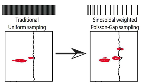
The Fourier transform has been the gold standard to transform data from time to frequency domain in many spectroscopic methods, including NMR. While reliable, it has as a drawback that it requires a grid of uniformely sampled data points, which is not efficient for decaying signals, while it also suffers from artifacts when dealing with non-decaying signals. Over several decades many alternative sampling and transformation schemes have been proposed. Their common problem is that relative signal amplitudes are not well preserved. Here we demonstrate superior performance of a sine-weighted Poisson gap distribution sparse sampling scheme, combined with FM reconstruction. While the relative signal amplitudes are well preserved, we also find that the signal-to-noise ratio is enhanced up to four fold per unit of data acquisition time as compared to the traditional linear sampling.

The capabilities of modern NMR spectrometers have recently improved dramatically due to higher magnetic field instruments. To utilize the potential resolution of these spectrometers in multi-dimensional experiments various forms of sparse or non-uniform sampling (NUS) were proposed^1,2. For optimal processing of such spectra we have recently developed the Forward Maximum entropy (FM) reconstruction method³, which was improved and combined with a distillation procedure⁴.

The quality of spectra obtained form NUS depends crucially on the sampling schedules. In the past we have examined various forms of random sampling and realized that the quality of data retrieval depended significantly on the choice of the seed number when using standard Unix random number generators (e.g. drand48). We realized that (1) big gaps in the sampling schedule are generally unfavorable, and (2) gaps at the beginning or end of the sampling are worse than in the middle. A third, crucial criterion is: (3) the sampling requires suitably random variation to prevent violation of the Nyquist theorem.

To cope with this we have evaluated a sinusoidal weighted Poisson distribution of the gap lengths between sampling points followed by FM reconstruction. To achieve this distribution, we assume an average gap length of λ in the common Fourier grid and a specific gap size k between two acquired data points. Thus, a λ of 0.0 yields uniform sampling, a λ of 1.0, for example, creates a non-uniform schedule of 50% overall sampling density.

The overall probability f for a specific gap size k ≥ 0 is assumed by the Poisson distribution: $f(k;\lambda )=\frac{{\lambda }^k{e}^{-\lambda }}{k!}$. This would satisfy the criteria (1) and (3). Obviously, no integer values k less than zero is allowed as no negative gap sizes are realizable.

To meet point (2) above, we further optimized the sampling schedule with a sinusoidal variation of λ and call this Sine-weighted Poisson-gap Sampling, SPS. Here λ = Λ sinθ, where Λ is the adjustment factor to keep the average λ to satisfy the targeted sampling density. θ spans linearly from 0 to π through the sampling schedule when no apodization is applied prior to reconstruction. As apodization commonly scales the signal to zero at the end of the evolution time, we restrict the variation of θ from 0 to π/2 when apodization is intended. The method intrinsically imposes some “order”, and sampling points are not chosen fully stochastically. The sinusoidal weighting of gap sizes is equivalent to very dense sampling at the beginning of the time domain data. This is ideal for exponentially decaying time domain data. For other data, such as anti-phase signals a different weighting may be optimal. A c-program for generating the SPS schedule is provided in the supplemental material.

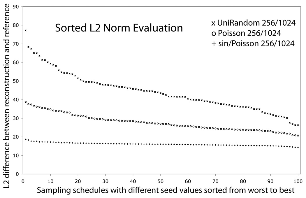
To test the performance of Poisson-gap sampling we generated a free-induction decay for a single resonance, tested different sampling schedules and examined how accurately the FM algorithm could reconstruct the signals. As an example, 256 out of 1024 time domain data points were extracted with different selection procedures. The data sets were then FM reconstructed and Fourier transformed without apodization. In particular we tested how the value of the Unix seed number affects the quality of the result. Fig. 1 shows a L² norm analysis of the accuracy of the reconstruction for 100 seed numbers. The L² values were ordered according to their size. The top trace is for plain random sampling, the middle trace uses Poisson-Gap sampling without modulation, and the lower trace uses Poisson-Gap sampling with a sinusoidal variation of λ (θ = [0,π]), SPS. Poisson-Gap sampling alone is almost two-fold better than plain random sampling, and SPS is by far the best. Importantly, it is almost completely insensitive to the choice of the Unix seed number. Thus, sinusoidal Poisson-Gap sampling is our method of choice for generating sampling schedules.

Figure 1.

Effect of Poisson-Gap sampling on the quality of spectra obtained with FM reconstruction. A synthetic time-domain signal (1024 data points) was created and 256 sampling points were selected with three different methods. The L² values, i.e the Euclidian norm ${\mathrm{L}}^2=\parallel \mathbf{f}-{\mathbf{f}}^{\mathbf{\text{rec}}}\parallel =\sqrt{{{\displaystyle \sum _{i=1}^n({\mathrm{f}}_{\mathrm{i}}-{\mathrm{f}}_{\mathrm{i}}^{\text{rec}})}}^2}$ or a non-normalized rmsd, of the difference between the reconstructed and the linearly sampled spectrum were calculated for 100 different Unix seed numbers, and ordered according to decreasing L² values. Top trace: plain random sampling Middle Trace: Poisson-Gap sampling without λ variation. Bottom trace: Poisson-gap sampling with a sinusoidal variation of λ (θ = [0,π]) The latter procedure clearly has the lowest L² values and is nearly independent of the seed number.

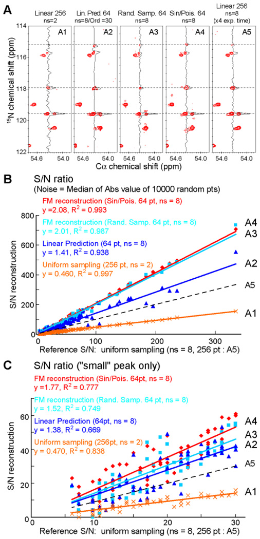
Next we examined experimentally the performance of Poisson-Gap sampling and FM reconstruction on a 2D ¹³Cα-detected NCa experiment on alternately ¹³C labeled B1 domain of protein G (GB1)⁵. We compared various sampling schedules and analyzed the effect on spectral quality, signal-to-noise ratio (S/N), recovery of very weak peaks, and fidelity of peak positions. Results are summarized in Fig. 2. A total of five NCa experiments were recorded and labeled A1–A5. Two NCa reference spectra of 256 uniformly sampled increments with 2 (A1) and 8 scans (A5) per increment were measured in 22 min and 1.5 hours, respectively. We then recorded three spectra with one quarter of the increments selected but accumulating 8 scans per increment. These required 22 min of measuring time each. These are: 64 first of 256 uniformly sampled increments (A2), 64 out of 256 increments random selected with uniform sampling density (A3), and 64 out of 256 selected by SPS with θ = [0,π/2] where Λ is adjusted by the schedule generator to create the requested number of sampling points (see supplement) (A4). The non-uniformly sampled spectra (A3 and A4) were subsequently FM reconstructed. The spectrum A2 that sampled the 64 first increments was linearly predicted to 256 time points using an order parameter of 30 (see supplement for the choice of this order parameter). The effective maximum nitrogen evolution time for all experiments was 84 ms, which is approximately 30% of the ¹⁵N T₂. A representative 2D strip with a cross section through the Cα position of residue 15 is used in Fig. 2A for comparison. The panels are labeled A1 to A5 to indicate the acquisition methods described above.

Figure 2.

Comparison of non-uniform sampling schedules with uniform acquisition and linear prediction. (A) A representative strip from the CαN spectrum⁵ of alternately ¹³C labeled protein GB1. The four strips at the left represent experiments of the same total measuring time (512 total scans). Strip 5 was recorded with 8 scans and 256 linear increments requiring a four-times longer experiment. For panel A2, the first 64 linear increments were extended with linear prediction using order parameter of 30. Panels 3 and 4 were obtained with a random sampling (64pts) and sine-weighted Poisson gap sampling (64 pts), respectively. B and C are plots of the S/N of all (B) and small (C) peaks, respectively. The S/N values of the picked peaks obtained with the procedures A1–A4 are plotted against A5.

Fig. 2B and 2C plot the S/N of all and only weak peaks, respectively. As signal we use the peak height, as noise the median of the absolute values of 10000 randomly picked spectral points. The S/N of A1–A4 is plotted against that of the spectrum recorded with the four-fold longer measuring time (A5) and fitted with linear regression. The linear coefficient shown in 2B and 2C represent the S/N relative to that of conditions A5, and the R² term reports the fidelity of reconstruction.

The data show that the S/N of A1 is approximately half (0.46 and 0.47 in 2B and 2C) of A5 since only one quarter of the scans was recorded. Plain random sampling and FM reconstruction (A3) yields a S/N relative to A5 of 2.01 and 1.52 for strong and weak peaks, respectively. SPS (A4) results in a S/N relative to A5 of 2.08 and 1.77 for strong and weak peaks, respectively. Thus, SPS combined with FM reconstruction performs best. Interestingly, the S/N of A4 is about four times higher than that of A1 although obtained in the same total measuring time, and it is about two times higher than that obtained with conditions of A5 although obtained in one quarter of the measuring time. Thus, the procedures described result in a significant gain in S/N per measuring time.

We then asked whether the procedure suffers from false positives. Indeed there are some weak peaks at 118.0 and 118.5 ppm in panel A4 and also a few weak peaks in panel A3. To explore this we selected ten areas of the spectrum that do not contain peaks and measured the signal to peak noise. The results are shown in Supplemental Figure S1 and indicate that Poisson-Gap sampling has also superior signal to peak noise, but to a smaller extent, particularly for small peaks.

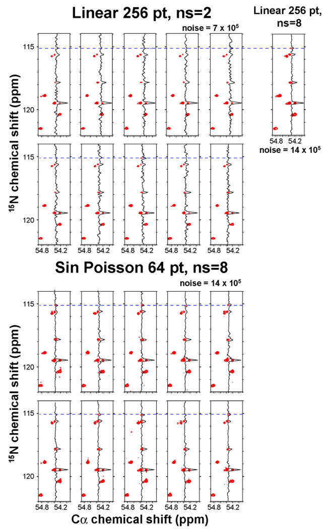
We then asked whether the small false positive peaks seen in Fig. 2, A3 and A4, are systematic or random artifacts. We recorded ten spectra with the conditions of Fig. 2A1 (256 linear increments, ns = 2), and ten spectra with the conditions of Fig. 2A4 (64 SPS increments, ns=8). The results are shown in Fig. 3. None of the false peaks show up reproducibly and are thus random artifacts; these are of minor concerns since peaks are typically not trusted unless they are seen reproducibly.

Figure 3.

Reliability of small peak detection. Top: The same NCa spectrum was recorded ten times linearly with 256 increments and two scans per increment. The same strip is shown as in Fig. 2 of the main manuscript. Bottom: The same NCa spectrum was recorded ten times with NUS recording 64 increments and eight scans per increment. The measuring time was 22 min for each of the experiments. Top right: For comparison, the spectrum was also recorded linearly with 256 increments and 8 scans per increment (total measuring time 1.5 hrs). The weak peak at the ¹⁵N chemical shift of 115.1 ppm, which is clearly manifested in the long linear experiment (1.5 hrs) is also clearly seen in the NUS spectra recorded in ¼ of the time (22 min). On the other hand, it is barely visible in only a few of the short linear experiments of 22 min.

Next we asked whether this NUS/FM reconstruction approach could enhance sensitivity. Here we define sensitivity as the ability to distinguish weak peaks from noise. As an example, the spectrum shown in Fig. 2A contains a weak peak at the nitrogen position of 115.1 ppm (marked at top with a dotted line. This peak could not be observed with linear sampling (Fig. 2A1); however, it is obvious and strong in the spectrum using SPS (A4) although both data sets used the same experimental time; it is better defined than in the spectrum A5 although recorded in only a quarter of the time. Thus, the SPS procedure described here, together with FM reconstruction seems to increases the sensitivity not just the S/N.

Is this sensitivity gain reproducible? To answer this we compare the uniformly and non-uniformly sampled spectra of Fig. 3. The figure shows cross sections and contour plots. The latter are drawn with two different noise levels. Noise level for spectra which recorded with ns=8 was set to be twice as high as the spectra recorded with ns=2, since the maximum noise value for ns=8 spectra (both uniformly and NUS sampled) were twice as high as in spectra with ns=2. Although it is somewhat subjective to decide whether a peak is there above the noise, the comparison of the spectra clearly shows that procedure A4 (Sine-weighted Poisson Gap sampling) consistently identifies the weak peak (Fig. 3 bottom panels, the peaks are obvious in 7/10 contour plots and the cross sections are always positive). But with procedure A1, the peaks are obvious only in 2/10 contour plots and the cross sections are even negative in some cases (Fig. 3 top panels). This clearly indicates better ability to distinguish signals from noise in the reconstructed spectra. Thus, the Poisson-Gap NUS and FM reconstruction enhances sensitivity, the ability to detect weak peaks above noise.

This sensitivity enhancement seems counter intuitive. However, one should keep in mind that the FM reconstruction is no transformation but a minimization procedure. Based on the design of the approach^3,4, the only experimental noise originates from the measured time-domain data points. Since we can measure here four times more scans than in the uniformly sampled data the signal to noise of the measured time-domain data points is two-fold higher. There is no experimental noise in the reconstructed data points. However, there is reconstruction noise due to the point-spread function (sampling schedule). We minimize this reconstruction noise by optimizing the sampling schedule and by the conjugant gradient optimization. Thus, it is possible to increase the signal-to-noise ration and the ability to enhance detection of weak signals above noise, which we consider an enhancement of the sensitivity.

We also compared the Poisson-gap sampling and FM reconstruction with linear prediction based on the first 64 linear increments (Fig. 2, A2). The S/N relative to A5 is 1.41 and 1.38 for strong and weak peaks, respectively. This is significantly better than A1 and even A5. However, we had to use a large order parameter of 30 in the nmrPipe program⁶. The benefits of using large order parameters in LP are discussed in detail in the supplemental material and in Fig. S2. However, linear prediction can cause small changes of peak positions as previously reported⁷ and is clearly seen for the peak at the nitrogen position of 115.1 ppm (top dotted line in Fig. 2 and Fig. S2). Such chemical shift changes are not observed in the SPS/FM reconstruction approach. Furthermore, linear prediction clearly suffers from significantly lower resolution, which matters for crowded spectral regions as shown in supplemental Fig. S3.

Currently, the Poisson-Gap sampling is only implemented in a single NUS dimension. However, implementation in multiple dimensions is possible and is currently being pursued.

References

- 1.Mobli M, Stern AS, Hoch JC. J Magn Reson. 2006;182:96–105. doi: 10.1016/j.jmr.2006.06.007. [DOI] [PubMed] [Google Scholar]
- 2.Kazimierczuk K, Zawadzka A, Kozminski W. J Magn Reson. 2008;192:123–130. doi: 10.1016/j.jmr.2008.02.003. [DOI] [PubMed] [Google Scholar]
- 3.Hyberts SG, Heffron GJ, Tarragona NG, Solanky K, Edmonds KA, Luithardt H, Fejzo J, Chorev M, Aktas H, Colson K, Falchuk KH, Halperin JA, Wagner G. J Am Chem Soc. 2007;129:5108–5116. doi: 10.1021/ja068541x. [DOI] [PMC free article] [PubMed] [Google Scholar]
- 4.Hyberts SG, Frueh DP, Arthanari H, Wagner G. J Biomol NMR. 2009;45:283–294. doi: 10.1007/s10858-009-9368-1. [DOI] [PMC free article] [PubMed] [Google Scholar]
- 5.Takeuchi K, Sun ZY, Wagner G. J Am Chem Soc. 2008;130:17210–17211. doi: 10.1021/ja806956p. [DOI] [PMC free article] [PubMed] [Google Scholar]
- 6.Delaglio F, Grzesiek S, Vuister GW, Zhu G, Pfeifer J, Bax A. J Biomol NMR. 1995;6:277–293. doi: 10.1007/BF00197809. [DOI] [PubMed] [Google Scholar]
- 7.Stern AS, Li KB, Hoch JC. J Am Chem Soc. 2002;124:1982–1993. doi: 10.1021/ja011669o. [DOI] [PubMed] [Google Scholar]
Associated Data
This section collects any data citations, data availability statements, or supplementary materials included in this article.