Automated detection of tuberculosis in Ziehl-Neelsen stained sputum smears using two one-class classifiers

Abstract

Screening for tuberculosis in high-prevalence countries relies on sputum smear microscopy. We present a method for the automated identification of Mycobacterium tuberculosis in images of Ziehl-Neelsen stained sputum smears obtained using a bright-field microscope. We use two stages of classification; the first implements a one-class pixel classifier, after which geometric transformation invariant features are extracted. The second stage employs one-class object classification. Different classifiers are compared; the sensitivity of all tested classifiers is above 90% for the identification of a single bacillus object using all extracted features. The mixture of Gaussians classifier performed well in both stages of classification. This method may be used as a step in the automation of tuberculosis screening, in order to reduce technician involvement in the process.

Background

Tuberculosis (TB) is caused by Mycobacterium tuberculosis, which enters the body through the lungs and which, expectorated in sputum, can be seen as clusters or individually in stained sputum smears under a microscope. Two staining methods are used: auramine, which requires fluorescence microscopy; and Ziehl-Neelsen (ZN), which requires bright-field microscopy.

The microscope is the cornerstone of TB screening in low- and middle-income countries (Steingart et al. 2006), as it is a relatively cheap piece of equipment. Positive sputum smear detection using a microscope makes up the largest fraction of total TB detections (WHO 2007). We concentrate on TB screening using a bright-field microscope, as this is the preferred method in developing countries, due to the low cost and ease of equipment maintenance compared to fluorescence microscopy; low-cost fluorescent microscopes have, however, recently become available (Hanscheid 2008).

TB screening with a conventional microscope has variable sensitivity; values between 20% and 60% have been reported in some studies, while sensitivity above 80% has been reported in others (Steingart et al. 2006). The WHO recommends that a slide be declared TB-negative if no bacilli are seen in 100 high-power microscope view fields (WHO 2003); a negative diagnosis, however, requires the examination of two or three negative smears. A technician normally examines between 30 and 40 smears in a day (Toman 2004) and may diagnose a positive slide as negative because of sparseness of bacilli, or because too few fields have been examined. In addition, the workload in high-prevalence countries leads to technician fatigue, diminishing the quality of microscopy (van Deun 2002).

Automation of microscopy for TB screening aims to speed up the screening process, to improve its sensitivity and to reduce its reliance on technicians. Automated detection of bacilli in sputum smear images is a step in the automation of TB screening microscopy

Pattern recognition techniques for the identification of TB were first proposed for auramine-stained sputum smears (Veropoulos et al. 1999; Forero et al. 2006). Veropoulos et al. (1999) filtered their captured images to detect object edges. Edge pixel linkage (Veropoulos et al. 1999) and morphological closing (Forero et al. 2006) have been applied to segmented objects to complete broken edge contours. Fourier descriptors have been used to describe segmented objects and sensitivity of 94.1% and specificity of 97.4% have been reported in the classification of objects using a feed-forward neural network with four hidden units (Veropoulos et al. 1999). Forero et al., (2006) segmented their captured images using an edge detection algorithm; Hu's moments were used to describe segmented objects. A minimum error Bayesian classifier was employed to classify objects. The classifier was unsupervised; it had as input clustered data and a threshold was drawn below which objects were classified as non-bacilli. Sensitivity of 97.89% and specificity of 94.67% was achieved in the classification of images, using a fixed threshold.

Santiago-Mozos et al. (2008) used pixel classification to find bacilli in images of auramine-stained sputum; they described each pixel by a square patch of neighbouring pixels and used principal component analysis to reduce the number of features – pixels – for input to a support vector machine classifier. Sadaphal et al. (2008) demonstrated proof of principle that colour-based Bayesian segmentation may be employed to extract TB bacilli in ZN-stained sputum smears.

We introduce one-class classifiers for the detection of TB in ZN-stained sputum smear images, in which acid-fast bacilli are red against a blue background. Bacilli have a waxy coating which absorbs the red of the Ziehl-Neelsen carbol fuchsin; the background is stained blue by the methylene blue counter-stain. We formulate the detection of TB as a novelty detection problem, as bacilli have a distinctive colour and shape. Remnants of cells, bacilli destroyed by macrophages and food particles are outlier objects. Novelty detection is applied to cases where the class of objects that are not of interest – outliers – cannot be sufficiently modelled (Bishop 1994) and is applied here because it is difficult to make an accurate ontology of the debris that may be present in a captured sputum smear image. The objects in the images are identified using two stages of classification. The aim is to identify individual bacilli (target objects), which are rod-shaped with varying curvatures and length between 1 and 10 μm (Forero et al. 2006), with their length in the focal plane of the image. The first stage uses colour information and pixel intensity values are used as features by classifiers. The second stage of classification uses shape information.

Methods

Image acquisition

A Nikon Microphot-FX microscope with a 100× oil objective, to which was attached a Kodak DC290zoom digital camera, was used for image acquisition. Pixel resolution was 720×480. Images were stored in JPEG file format, with 24 bits per pixel, in colour. The microscope was used without any filters; its halogen 12V, 100W lamp was set to 7-9V. Images were captured in a room with fluorescent lighting. Camera zoom was set at 65mm and exposure time at 0.1 seconds.

Nineteen ZN-stained sputum smear slides from 19 different subjects were prepared by the South African National Health Laboratory Services (NHLS) at Groote Schuur Hospital in Cape Town. All the slides were confirmed as smear positive by technicians at the NHLS. Between 20 and 100 images of different microscope fields were taken per slide. Among images that demonstrated adequate staining and the presence of bacilli, training and test sets were chosen randomly.

Pixel classifiers for object segmentation

The first stage of classification uses one-class pixel classifiers to identify candidate bacillus objects using colour information. Gaussian, mixture of Gaussians (MoG), and principal component analysis (PCA) classifiers are used. For the Gaussian classifier, the target class is modelled as a Gaussian distribution, and objects with features falling outside a threshold are labelled as outliers. The mixture of Gaussians classifier uses a number of Gaussians to create a more robust description of the target class (Bishop 1995). The PCA one-class classifier allows a choice of the eigenvectors of the target data covariance matrix to be used in describing the target data; removing high variance eigenvectors usually improves performance for data with low dimensionalities (Tax & Muller, 2003).

As pixel classification relies on pixel colour, the colour space used in classification may influence the accuracy of the results. The performance of the classifiers on different colour spaces was examined, so as to select the colour space that produced the best results.

Classifier training

Usually, the outliers of a one-class classifier cannot be sufficiently sampled, therefore their training involves setting a percentage error a classifier may make during training; the percentage error defines the number of target objects that may be misclassified as outlier objects. One-class classifiers form a closed decision boundary around the target data points. There is a trade-off between rejected target objects and accepted outliers. To compare performance of classifiers on a test set, the same allowable percentage of error is specified on the training target set for the different classifiers. The function derived using the set percentage of error on target objects is used to classify the test dataset.

Evaluation of stage one classifiers

Stage one of the bacillus identification method outputs image objects with the colour of TB bacilli. An evaluation procedure that uses a manually segmented reference image to provide true or false classification rates was used to assess stage one classifiers (Meurie et al. 2003). The common and difference rates are found: the common rate is the number of pixels that are correctly classified; the difference rate is the number of pixels that belong to bacilli in the reference image that are not identified as the same class in the segmented image as well as pixels that belong to background in the reference image identified as object pixels in the segmented image. For each class, the common rate is averaged by the object pixels in the reference image to give the percentage of correctly classified pixels; the difference rate is averaged by the union of the reference image object pixels and the classified image object pixels to give the percentage of incorrectly classified pixels.

Stage two classification

Objects output by the first stage of identification are filtered based on their area; the threshold was set at a minimum of 50 pixels and a maximum of 400 pixels. The second stage of classification refines the results of the first stage by using shape information. In the second stage, the isolated candidate bacillus objects retained after filtering are the target class of the one-class classification; the rest of the objects picked up by stage one classifiers are outliers. Outliers are mainly composed of touching bacilli, remnants of cells or food particles. The classifiers in the two stages are all supervised learning algorithms.

The numbers of target and outlier objects extracted from the first stage of classification are used as priors in the second stage. All the stage one classifiers are used in the final stage classification. Additionally, the k-nearest neighbour (kNN) classifier is used (Duda et al. 2001). MoG and Gaussian classifiers are density based; the kNN classifier describes the boundary of the target class and the PCA one-class classifier is a reconstruction classifier – it reconstructs object parameters using low variance eigenvectors (Tax & Muller 2003).

Feature extraction

Features were extracted from the objects retained from stage one after filtering based on area, and the performance of classifiers was compared for different feature sets. The 2-dimensional coordinates of the boundary pixels of an object form a closed shape; if the second value of each of the K coordinates is made imaginary, the discrete Fourier transform of the coordinates s(k) is

$$a(u)={\sum }_1^{K-1}s(k)e^{\frac{-j\pi 2uk}{K}}.$$

The complex coefficients a(u), u = 0, 1, 2…K-1, are used as Fourier features (Gonzalex et al. 2004). Fourier features can be made invariant to translation and rotation using the transform: $r(u)=\sqrt{|a_x(u){|}^2+|a_y(u){|}^2}$, where a_x(u) and a_y(u) are the real and imaginary parts of the coefficients or descriptors. Since Fourier features are translation and rotation invariant, they were compared to moment invariant features which are also geometric change invariant. The moment features are derived from the generalised colour moment (Mindru et al. 2004). The last feature set used in the comparisons consists of eccentricity, the ratio of the major and minor axes of an object, and compactness, which provides a measure of how closely the shape of the object approaches a circle and is the ratio of the perimeter and area of the object. Eccentricity and compactness are useful descriptors because of the long and thin rod-like shape of bacilli.

Linear Fisher mapping was applied to the set of all extracted features; it reduces the dimensionality of the feature space based on the optimisation of the between-class scatter matrix S_b with respect to the within class scatter matrix S_w (Franco et al. 2006): $S_b={\sum }_{i=1}^m{P}_i(u_i-u_o){(u_i-u_o)}^T$ with respect to $S_w={\sum }_{i=1}^m{P}_i{S}_i$

For each of the m classes, S_i is the covariance matrix, P_i is the prior probability, u_i is the class mean and u_o is the global mean vector.

The second stage dataset is normalised so that no feature dominates in the decision making, by subtracting the mean of each feature from each feature element, then dividing each feature element by the standard deviation of that feature.

Evaluation of stage two classifiers

Sensitivity and specificity of a classifier can be combined for a better picture of classifier performance by using receiver operating characteristics (ROC) (Gonzalex et al. 2004). The ROC space is two dimensional, thus classifiers can be compared or evaluated by a point in the plane. The ROC curve (sensitivity against 1-specificity) is obtained by varying the classifier threshold between its extremes. Points on the curve closest to the upper left corner of the ROC space correspond to classifier parameters that yield good performance. The area under an ROC curve is a robust error measure for one-class classification (Metz 1978).

Results

Stage one classification

The dataset of images used to train pixel classifiers was derived from nine subjects and was composed of 28 images, from which pixels of bacilli in the focal plane were labelled manually as target objects. A subset of background pixels was labelled as outliers. The objects of the training dataset had three features – the pixel values of the three channels of a colour space. The dataset contained 40666 objects, of which 20637 were bacillus objects.

The classifiers were assessed using a dataset of 20 images from different subjects. Each image had a manually segmented version used to calculate the ratios of correctly and incorrectly classified pixels. Table 1 shows these ratios, which were used to rank pixel classifiers in order of segmentation accuracy, and investigate which colour space is best suited for the pixel classifier segmentation method.

Table 1. Performance of pixel classifiers; ratios of correctly (top figure) and incorrectly (bottom figure) classified pixels in different colour spaces.

		Colour Space
		RGB	HSV	YCbCr	CIE-Lab
Classifier	Gaussian	0.7846 0.3968	0.8544 0.9876	0.7852 0.3952	0.7808 0.3968
	MoG	0.8893 0.3163	0.8797 0.5551	0.8891 0.3331	0.8903 0.3652
	PCA	0.7012 0.6190	0.6941 0.9747	0.6875 0.7040	0.7203 0.7891
	Average	0.7917 0.4440	0.8094 0.8391	0.7873 0.4774	0.7971 0.5170

The RGB colour space had the best performance across different classifiers. For all classifiers, it had the lowest percentage of incorrectly classified pixels. The mixture of Gaussians classifier performed best. Figure 1 shows an example of the results produced by the first stage of classification.

Figure 1. Results of the MoG pixel classifier overlaid on a sub-image of the test dataset.

Stage two classification

The classification accuracy of the k-nearest neighbour classifier was used to determine the number of Fourier coefficients to use – 14. Moment invariants, eccentricity and compactness were also used to describe objects. The training dataset consisted of 4376 objects from nine subjects; 2728 objects were labelled as target objects and 1648 were labelled outliers. All classifiers were tested using a dataset from eight subjects with 1064 objects labelled as target objects and 1157 objects labelled as outliers. Figure 2 shows example outlier objects; some of these are clumps of touching bacilli, which have lost the characteristic shape exploited during classification. Table 2 shows the performance of different classifiers on different features, all evaluated at their best operating point. The area under an ROC for these classifiers is shown in Table 3. Tables 4 and 5 show the performance of classifiers on the full set of extracted features and on the linear Fisher mapped feature set.

Figure 2. Example outlier objects; (a) clumps of touching bacilli; (b) red stains.

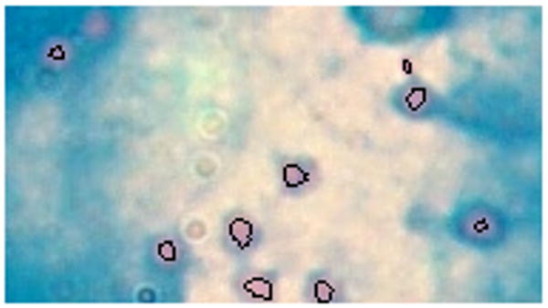
Table 2. Performance of classifiers using different feature sets.

	Classifier		Accuracy (%)
			Sensitivity (%)
			Specificity (%)
	Gaussian	MoG	PCA	kNN
Fourier features	73.75	84.33	71.68	71.41
	90.32	90.51	92.29	92.20
	58.51	78.65	52.72	52.29
Moment invariants	51.91	50.88	50.47	50.74
	94.55	94.36	95.49	94.83
	12.71	10.89	9.08	10.20
Eccentricity and compactness	85.59	90.18	90.81	87.12
	94.36	98.21	98.59	93.99
	77.53	82.80	83.66	80.81

Table 3. Evaluation of classifiers on different feature sets using the area under the ROC curve.

	Gaussian	Mixture of Gaussians	PCA	kNN
Fourier features	0.8152	0.9232	0.7583	0.7933
Moment invariants	0.5944	0.5766	0.5931	0.5437
Eccentricity compactness	0.9044	0.9509	0.9154	0.9065

Table 4. Performance of classifiers using the set of all features.

	Classifier		Accuracy (%)
			Sensitivity (%)
			Specificity (%)
	Gaussian	Mixture of Gaussians	PCA	kNN
Set of all extracted features	85.59	93.47	81.00	78.12
	91.07	90.88	90.88	94.08
	80.55	95.85	71.91	63.44
Linear Fisher mapping	90.63	89.78	47.91	90.68
	84.40	81.49	100	84.40
	96.37	97.41	0	96.46

Table 5. Evaluation of classifiers on all features using the area under the ROC curve.

	Gaussian	Mixture of Gaussians	PCA	kNN
Set of all extracted features	0.9424	0.9810	0.9069	0.8934
Linear Fisher mapping	0.9759	0.9801	0.5000	0.9748

Discussion

The aim of our study was to detect TB bacilli in ZN-stained sputum smears, using an algorithm comprising segmentation of candidate bacillus objects and classification of segmented objects. We use one-class classification for both stages.

A two-class classifier learns the two classes; for example, Veropoulos et al. (1999) used artificial neural networks, and Santiago-Mozos et al. (2008) used support vector machines, which draw a hyperplane to separate bacillus and non-bacillus objects. One-class classifiers only learn the class of interest, drawing a closed boundary around it, and hence are less prone to effects of outliers than are two-class classifiers. However, two-class classifiers can have higher accuracy than one-class classifiers for a well-sampled problem, because one-class classifiers are designed to misclassify a certain percentage of target objects in order to have high specificity. For ZN-stained sputum smears, the red rod-like bacilli are easy to learn compared to non-bacillus objects. Non-bacillus objects are mostly touching bacilli, and out-of-focus objects that have lost the hue of the colour red.

Sadaphal et al. (2008) segmented ZN-stained sputum smear images, but did not provide quantitative results. They extracted two shape descriptors from the objects, axis ratio and eccentricity, and thresholded them to find a range for TB bacilli. For segmentation, we use a similar procedure for training the pixel classifier; the RGB values of pixels are used as objects. But for the last stage of identification we train object classifiers as opposed to thresholding object features to find the range for bacillus objects. Santiago-Mozos et al. (2008) classified patches of pixels in auramine images as to whether or not they contained bacilli; they performed sequential tests on detected patches until set false alarm and detection probabilities were met.

The mixture of Gaussians performed best in the first stage of classification. It showed the lowest ratio of incorrectly classified pixels, which translates into few outlier pixels classified as bacilli. It picked up most of the bacilli with their length in the focal plane of an image; the relatively low percentage of correctly classified pixels – 88.93% – was mainly due to inaccuracy in detecting object outlines. The mixture of Gaussians is a density based classifier. The dataset had three features; therefore density estimation was less complicated due to low dimensionality.

Crystallized red stain deposits, possibly due to the delay in washing off the Ziehl-Neelsen carbol fuchsin with the acid alcohol used to decolorize the slide, were a source of segmentation error. Figure 2 (b) shows red stains that were picked up by the first stage of identification. Focus of the microscope also negatively affected the first stage of identification; Figure 3 shows that the method had difficulty picking up out-of-focus bacilli.

Figure 3. Results of the MoG pixel classifier on an image with out-of-focus bacilli.

The Gaussian and mixture of Gaussians classifiers performed best in the second stage of classification, using all features. While using eccentricity and compactness alone provided high sensitivity for all classifiers (Table 2), the addition of Fourier features and moments increased the specificity of classification for the Gaussian and mixture of Gaussian classifiers. Since individually the moment features had worse specificity than Fourier features, the improvement can be attributed to Fourier features. The PCA classifier performed poorly on the linear Fisher mapped test set because it requires variance of features, which is removed by Fisher mapping. Fisher mapping improved specificity but reduced sensitivity for the other classifiers.

Pixel classifiers resulted in fewer outlier objects than would have been produced by conventional low-level image processing techniques. Thus the number of target and outlier objects extracted from the first stage of classification could be used as priors in the second stage; objects presented to the classifiers for the final identification step were more likely to be target than outlier objects. Images containing much debris or which were poorly stained were likely to produce more outlier objects than target objects, but such images were not used for either training or testing classifiers.

Further work may be done to probe the performance of classifiers on different settings on the ROC curve. The classifier results presented were calculated on the point on the ROC curve established by cross-validation. Classifiers could be tested on a point on the ROC curve with higher sensitivity and lower specificity, by changing the threshold on the posterior probabilities returned by object classifiers, to maximise detection of positive cases. Subsequent steps in the screening process may be used to detect the false positives.

The sensitivities and specificities we have obtained for one-class classifiers with images from bright-field microscopy are lower than those reported for fluorescence microscopy (Veropoulos et al. 1999). This is consistent with manual screening, which performs more poorly on ZN-stained sputum: a systematic review by Steingart et al. (2006) revealed that fluorescence microscopy is on average 10% more sensitive than bright-field microscopy in detecting TB in sputum smears.

Misclassification of individual bacilli in a sample or slide with a high bacillus count will have little influence on a final diagnosis based on a threshold number of individual bacilli in the entire sample. Thus correct classification of every bacillus in a slide is not required for an automated system to be useful. Forero et al. (2006) obtained sensitivity and specificity of 97.89% and 94.67%, respectively, when classifying images or fields of auramine-stained sputum using a pattern recognition algorithm; they found sensitivity and specificity of 100% when detecting a minimum of two or three bacilli in an entire slide, using the same algorithm. Realistic assessment of the diagnostic utility of an automated system by comparing it with manual microscopy, requires the use of a slide or sample as the unit of analysis. Such a comparison can only be made after development of a fully automated slide analysis system, incorporating automatic focusing, stage movement, image capture and image analysis, all under computer control.

Conclusions

We have shown that one-class classifiers are able to detect bacilli in sputum smear images with high accuracy; the classifiers exploit the colour and shape features of bacilli, and novelty-detection confers flexibility in dealing with non-bacillus pixels and objects. The methods presented may be useful in improving the sensitivity of conventional microscopy for TB screening: screening is normally done on a population containing more negative than positive cases (WHO 2007); a technician would therefore have to examine a large number of additional fields to improve the detection of TB cases by a small fraction, risking fatigue and lowering the rate of processing of samples. However, a computer is able to process a large number of microscope view fields without these limitations.

References

- Bishop C. Neural Networks for Pattern Recognition. Oxford University Press; Oxford: 1995. [Google Scholar]
- Bishop C. Novelty detection and neural network validation. IEE Proceedings on Vision, Image and Signal Processing. Special Issue on Applications of Neural Networks. 1994;141:217–222. [Google Scholar]
- Duda R, Hart P, Stork D. Pattern Classification. John Wiley; New York: 2001. [Google Scholar]
- Forero M, Cristobal G, Desco M. Automatic identification of Mycobacterium Tuberculosis by Gaussian mixture models. Journal of Microscopy. 2006;223:120–132. doi: 10.1111/j.1365-2818.2006.01610.x. [DOI] [PubMed] [Google Scholar]
- Franco A, Lumini A, Maio D, Nanni L. An enhanced subspace method for face recognition. Pattern Recognition Letters. 2006;27:76–84. [Google Scholar]
- Gonzalez R, Woods R, Eddins S. Digital Image Processing Using MATLAB. Pearson Prentice Hall; New Jersey: 2004. [Google Scholar]
- Hanscheid T. The future looks bright: low-cost fluorescent microscopes for detection of Mycobacterium tuberculosis and Coccidiae. Transactions of the Royal Society of Tropical Medicine and Hygiene. 2008;102:520–521. doi: 10.1016/j.trstmh.2008.02.020. [DOI] [PubMed] [Google Scholar]
- Metz C. Basic Principles of ROC Analysis. Seminars in Nuclear Medicine. 1978;8:283–298. doi: 10.1016/s0001-2998(78)80014-2. [DOI] [PubMed] [Google Scholar]
- Meurie C, Lebrun G, Lezoray O, Elmoataz A. A comparison of supervised pixel-based colour image segmentation methods. Application in Cancerology. WSEAS Trans on Computers. 2003;2:739–744. [Google Scholar]
- Mindru F, Tuytelaars T, Van Gool L, Moons T. Moment invariants for recognition under changing viewpoint and illumination. Computer Vision and Image Understanding. 2004;94:3–27. [Google Scholar]
- Sadaphal P, Rao J, Comstock G, Beg M. Image Processing Techniques for Identifying Mycobacterium Tuberculosis in Ziehl-Neelsen Stains. Int J of Tuberculosis and Lung Disease. 2008;12:579–582. [PMC free article] [PubMed] [Google Scholar]
- Santiago-Mozos R, Fernandez-Lorenzana R, Perez-Cruz F. On the uncertainty in hypothesis testing. Proc. of the 5th IEEE Symposium on Biomedical Imaging: from Nano to Macro; 2008. pp. 1223–1226. [Google Scholar]
- Steingart K, Henry M, Ng V, Hopewell P, Ramsay A, Cunningham J, Urbanczik R, Perkins M, Aziz M, Pai M. Fluorescence versus conventional sputum smear microscopy for tuberculosis: a systematic review. Lancet Infectious Diseases. 2006;6:570–581. doi: 10.1016/S1473-3099(06)70578-3. [DOI] [PubMed] [Google Scholar]
- Tax D, Muller K. Feature extraction for one-class classification. Proc. of the International Conference on Artificial Neural Networks and Neural Information Processing; Istanbul. 2003. pp. 342–349. [Google Scholar]
- Toman K. What are the advantages and disadvantages of fluorescence microscopy? In: Frieden T, editor. Toman's tuberculosis: case detection, treatment, and monitoring—questions and answers. World Health Organization; Geneva: 2004. pp. 31–34. [Google Scholar]
- Van Deun A, Salim A, Cooreman E, Hossain M, Rema A, Chambugonj N, Hye M, Kawria A, Declercq E. Optimal tuberculosis case detection by direct sputum smear microscopy: how much better is more? International Journal of Tuberculosis and Lung Diseases. 2002;6:222–230. [PubMed] [Google Scholar]
- Veropoulos K, Learmonth G, Campbell C, Knight B, Simpson J. Automated identification of tubercle bacilli in sputum - a preliminary investigation. Analytical and Quantitative Cytology and Histology. 1999;21:277–281. [PubMed] [Google Scholar]
- World Health Organisation: Tuberculosis Fact Sheets. 2007 http://www.who.int/mediacentre/factsheets/fs104/en/
- World Health Organisation: Supporting Laboratory Services. 2003 http://whqlibdoc.who.int/hq/2003/WHO_CDS_TB_2002.310_mod9_eng.pdf.