Discriminative learning for protein conformation sampling

Abstract

Protein structure prediction without using templates (i.e., ab initio folding) is one of the most challenging problems in structural biology. In particular, conformation sampling poses as a major bottleneck of ab initio folding. This article presents CRFSampler, an extensible protein conformation sampler, built on a probabilistic graphical model Conditional Random Fields (CRFs). Using a discriminative learning method, CRFSampler can automatically learn more than ten thousand parameters quantifying the relationship among primary sequence, secondary structure, and (pseudo) backbone angles. Using only compactness and self-avoiding constraints, CRFSampler can efficiently generate protein-like conformations from primary sequence and predicted secondary structure. CRFSampler is also very flexible in that a variety of model topologies and feature sets can be defined to model the sequence-structure relationship without worrying about parameter estimation. Our experimental results demonstrate that using a simple set of features, CRFSampler can generate decoys with much higher quality than the most recent HMM model.

Introduction

Various genome sequencing projects have led to the identification of millions of proteins. To fully understand the biological functions and functional mechanisms of these proteins, the knowledge of their three-dimensional structures is essential. Many protocols and programs have been developed to predict the structure of a protein from its primary sequence. Roughly, these protocols can be categorized into two groups: template-based modeling and template-free modeling (i.e., ab initio folding). Template-based modeling methods can give a reasonable prediction for approximately 60–70% of new proteins.¹ Ab initio folding has made exciting progress in the past decade, as exemplified by the fragment assem bly method implemented in Rosetta.² However, ab initio folding still faces many formidable challenges in both conformation sampling and energy function design. The subject of this article lies in protein conformation sampling, that is, the exploration of the conformational space compatible with a given protein sequence. In particular, we first develop a Conditional Random Fields (CRF) model, called CRFSampler, to learn the complicated relationship between protein sequence and structure and then sample the conformations of a protein using this CRF model. CRFSampler models the sequence-structure relationship using more than ten thousand parameters and estimates them using a sophisticated discriminative learning method.

The fragment assembly method for protein conformation sampling has achieved great success in recent CASP events.^1,3,4 For example, two top methods in CASP7, Rosetta² and Zhang-server⁵, both use fragment assembly. Many other groups^6–13 have also developed fragment-assembly-based structure prediction methods and demonstrated success. Fragment based protein structure prediction is done in two steps: (1) cut a protein sequence into many small sequence segments and then identify dozens of candidate fragments (i.e., building blocks) for each sequence segment; and (2) construct the protein structure with those building blocks using some search or simulation algorithms. Although the fragment assembly method demonstrates promising results, several important issues remain with this method. First, because of the limited number of experimental protein structures in PDB, it is still very difficult to have a library of even moderate-sized fragments that can cover all the possible local conformations of a sequence stretch. Second, the conformational space defined by a fragment library is discrete, which is inconsistent with the continuous characteristics of protein backbone torsion angles. This discrete nature may restrict the search space and cause loss of prediction accuracy. To make the conformational space continuous, Bystroff et al. have developed HMMSTR,¹⁴ a Hidden Markov Model (HMM) model trained from a fragment library, to generate local conformations for a sequence stretch.

Two recent articles,^15,16 have studied if the backbone structure of a protein can be rebuilt supposing that its (ϕ, Ψ) angles are restricted to their native Ramachandran basins. A native Ramachandran basin is the region that a pair of native backbone torsion angles (ϕ, ψ) lies in. Sosnick and coworkers¹⁶ partitioned the torsion angle space into six regions (see Fig. 1 in Ref. 16) while Gong et al.¹⁵ divided the (ϕ, ψ) angle space into 36 regions (see Fig. 1 in Ref. 15). Both articles have demonstrated that if the angles are restrained to their native basins, then the backbone structure of many small-sized proteins can be rebuilt with a good accuracy. Although these studies are not pure ab initio folding, they indicate that if we can correctly guess the native basins of all the (ϕ, ψ) angles, then we should be able to predict well the backbone structure of a protein.

Very recently, Hamelryck et al. have developed an HMM model¹⁷ to sample protein conformations from a continuous space. The method uses a Hidden Markov Model to predict the native basins of a protein sequence by learning the local sequence-structure relationship. The strength of this method lies in two aspects: (1) this method models the backbone angles using a directional statistics distribution^18–20 so that they can be sampled from a continuous space; and (2) the HMM model can capture the dependency between two adjacent backbone angles. Experimental results demonstrate that by modeling dependency between two adjacent positions, the HMM model can generate more native-like conformations than this correlation is not modeled. Several fragment assembly methods^14,21 also exploit the dependency between two adjacent fragments and illustrate that this kind of dependency is very helpful for conformation sampling.

Experimental results indicate that the HMM sampling method¹⁷ is promising, but the HMM model is based on several assumptions that can be relaxed. The first assumption is that the residue at one position is independent of its secondary structure type, which contradicts with the fact that an amino acid has some preference to a certain secondary structure type. Second, the HMM sampling method also assumes that the hidden state (i.e., the distribution of backbone angles) at position i only directly depends on the residue and secondary structure at position i. This contradicts with the finding in Ref. 22 that the angles at position i depends on at least the three residues at positions i−1, i and i+1. These two assumptions are necessary in Ref. 17 because the HMM parameters are estimated by maximizing P(A, X, S), the joint probability of primary sequence A, secondary structure X and hidden states S (i.e., angles). To estimate P(A, X, S),^* these assumptions have to be made to deal with the sparsity in the training data and avoid overfitting. Given the sparsity in the training data, it is also very hard to incorporate more complexity into the HMM model without raising the risk of overfitting, which restricts the expressive power of the HMM model. In fact, this is a common problem of all the generative learning methods (e.g., HMM) that optimize the joint probability of states and observations.^23† Instead, discriminative learning methods such as CRFs can be more expressive and at the same time keeping the risk of overfitting under control. Discriminative learning is different from generative learning in that the former one optimizes the conditional probability of states on the observations while the latter one the joint probability of states and observations.

This article presents CRFSampler, an extensible and fully automatic framework, for effective protein conformation sampling, based on a probabilistic graphical model Conditional Random Fields.^24,25 Similar to the HMM model,¹⁷ CRFSampler samples backbone angles from a continuous space using sequence and secondary structure information. CRFSampler also models the dependency between the angles at two adjacent positions. CRFSampler differs from the HMM model in the following aspects. First, CRFSampler is more expressive than the HMM model. The backbone angles at position i can depend on residues and secondary structures at many positions instead of only one. In CRFSampler, a sophisticated model topology and feature set can be defined to describe the dependency between sequence and structure without worrying about learning of model parameters. Different from the HMM model, in which the model complexity (hence risk of overfitting) roughly equals to the number of parameters in the model, the effective complexity of CRFSampler is regularized by a Gaussian prior of its parameters, allowing the user to achieve a balance between model complexity and expressivity. Second, CRFSampler does not assume that primary sequence is independent of secondary structure in determining backbone angles. Instead, CRFSamler can automatically learn the relative importance of primary sequence and secondary structure. Final, CRFSampler can easily incorporate sequence profile (i.e., position-specific frequency matrix) and predicted secondary structure likelihood scores into the model to further improve sampling performance. Our experimental results demonstrate that, using only compactness and self-avoiding constraints, CRFSampler can quickly generate more native-like conformations than the HMM model and best decoys closer to their natives.

Methods

Backbone conformation representation and modeling

A protein backbone conformation can be described by three angles ϕ, ψ, ω, and a set of bond lengths^‡. Since the bond lengths and ω can be approximated as constants, we can represent a protein backbone as a set of (ϕ, ψ) angles. Except the two terminal residues of a protein chain, each residue has a pair of ϕ and ψ angles. Once we have such a set of (ϕ, ψ) angles, we can calculate coordinates for all the nonhydrogen atoms of a protein backbone. However, for some proteins, even if we have all of their native ϕ and ψ angles, we cannot accurately rebuild their backbone conformations because of slight variation of other angles.

Instead of the (ϕ, ψ) representation, this article employs another representation of a protein backbone. A protein backbone can be represented as a set of pseudoangles (θ, τ)²⁶ since the virtual bond length between two adjacent C_α atoms can be approximated as a constant (i.e., 3.8 Å).^§ In this representation, only the C_α atoms are take into consideration and other atoms are ignored. For any position i in a backbone, θ is defined as the pseudobond angle formed by the C_α atoms at positions i−1, i and i+1; τ is a pseudo dihedral angle formed by the C_α atoms at positions i−2, i−1 i and i+1. Given the coordinates of the C_α atoms at positions i−2, i−1, and i, the coordinates of the C_α atom at position i+1 can be calculated from (θ, τ) at position i. Therefore, given the positions of the first three C_α and N−2 pairs of (θ, τ), we can build the C_α trace of a protein. The relative positions of the first three C_α atoms are determined by the θ angle of the second residue. Using (θ, τ) representation, only the coordinates of the C_α atoms can be recovered. The coordinates of other backbone atoms and C_β atom can be built using programs such as MaxSprout,²⁷ BBQ,²⁸ and SABBAC,²⁹ which can build backbone positions with RMSD less than 0.5 Å.

The preferred conformations of an amino acid in the protein backbone can be described as a probabilistic distribution of the θ and τ angles. Each (θ, τ) corresponds to a unit vector in the three-dimensional space (i.e., a point on a unit sphere surface). We can use the 5-parameter Fisher-Bingham (FB5) distribution^17,18 to model the probability distributions over unit vectors. FB5 is the analogue on the unit sphere of the bivariate normal distribution with an unconstrained covariance matrix. The probability density function of the FB5 distribution is given by

$$f(u)=\frac{1}{c(\kappa ,\beta )}\text{exp}(\kappa {\gamma }_1\cdot u+\beta ({({\gamma }_2\cdot u)}^2-{({\gamma }_3\cdot u)}^2))$$ (1)

where u is a unit vector variable and c(κ,β) is a normalizing constant.¹⁸ The parameters κ (>0) and β (0 < 2β ≤ κ) determine the concentration of the distribution and the ellipticity of the contours of equal probability, respectively. The higher the κ and β parameters, the more concentrated and elliptical the distribution is, respectively. The three vectors γ₁, γ₂, and γ₃ are the mean direction, the major and minor axes, respectively. The latter two vectors determine the orientation of the equal probability contours on the sphere, while the first vector determines the common center of the contours.

CRF model

CRF model for sequence-structure relationship

Conditional random fields (CRFs) are probabilistic graphical models that have been extensively used in modeling sequence data. Please refer to Refs. 24 and ²⁵ for a complete description of CRFs. Here, we describe how to predict the backbone angles of a protein from its primary sequence and secondary structure using CRFs. In this context, the primary sequence and secondary structure of a protein are called observations and its backbone angles are hidden states or labels.

Let o = {o₁, o₂,…,o_N} denote an observation sequence of length N where o_i is an observed object. Each observed object can be a residue or a secondary structure type or their combination. Let S = {h₁,h₂,…,h_c} be a finite set of labels (also called states), each representing a distribution of backbone angles. Let s = {s₁,s₂,…,s_N} (s_i ∈ S) be a sequence of labels corresponding to the observation o. As opposed to the HMM model¹⁷ defining a joint probability of the label sequence s and the observation o, our CRF model defines the conditional probability of s given o as follows.

$$P_{\theta }(s|o)=\text{exp}\left(\sum _{i=1}^{N}F(s,o,i)\right)/Z(o)$$ (2)

where θ = (λ₁,λ₂,…λ_p) is the model parameter and $Z(o)={\sum }_s\text{exp}\left({\sum }_{i=1}^{N}F\left(s,o,i\right)\right)$ is a normalization factor summing over all the possible label sequences for a given observation sequence. F(s,o,i) is the sum of the CRF features at sequence position i:

$$F(s,o,i)=\sum _k{\lambda }_k{e}_k(s_{i-1},s_i)+\sum _l{\lambda }_l{\nu }_l(o,s_i)$$ (3)

where e_κ(s_i−1,s_i) and ν_l(o,s_i) are called edge and label feature functions, respectively.

The edge and label functions are defined as

$$e_k(s_{i-1},s_i)=\left[s_{i-1}=h_1\right]\left[s_i=h_2\right]$$ (4)

and

$${\nu }_l\left(o,s_i\right)=[x_l(o,i)][s_i=h],$$ (5)

where s_i = h indicates that the label (or state) at position i is h. And x_l(o, i) is a logical context predicate indicating whether or not the context of the observation sequence o at position i holds a particular property or fact of empirical data. [f] is equal to 1 if the logical expression f is true, and zero otherwise. Note that we can also define the edge feature function e_k(s_i−1, s_i) as [x_l(o, i)] [s_i−1 = h₁] [s_i = h₂], to capture relationship between two adjacent labels and observations. By expanding Eq. (2) using Eq. (3), (4), and (5) and merging the same items, the conditional probability can also be reformulated as follows.

$$P_{\theta }\left(s|o\right)=\frac{\text{exp}\left({\sum }_{i=1}^{q}F\left(s,o,i\right)\right)}{Z\left(o\right)}=\frac{\text{exp}\left({\sum }_k{\lambda }_k{C}_k\left(s,o\right)\right)}{{\sum }_s\text{exp}\left({\sum }_k{\lambda }_k{C}_k\left(s,o\right)\right)}$$ (6)

Where C_k(s,o) represents the occurring times of the kth feature in a pair of label sequence s and observation sequence o and the model parameter λ_k is the weight of this feature. Here, the parameter λ_k does not correspond to the log probability of an event (as in the HMM model¹⁷) Instead, it is a real-valued weight that either raises or lowers the “probability mass” of s relative to other possible label sequences. The parameter λ_k can be negative, positive, or zero.

The CRF model is more expressive than the HMM model in Ref. 17. First, we do not have to interpret the parameter λ_k as the log probability of an event. Second, CRFs do not have to assume that the observation object at one position is independent of other objects. That is, for any ν_l(o,s_i), the label at position i can depend on many observed objects in the observation sequence or even the whole observation sequence. In addition, s_i can also depend on any nonlinear combination of several observed objects. Therefore, the CRF model can accommodate complex feature sets that may be difficult to incorporate within a generative HMM model. The underlying reason is that CRFs only optimize the conditional probability P_θ(s|o) instead of joint probability P_θ(s,o), avoiding calculating the generative probability of the observation sequence.

Model parameter estimation

Given a set of observation sequences and their corresponding label sequences (oⁱ, sⁱ), CRFs train its parameter θ = {λ₁,λ₂,…,λ_p} by maximizing the conditional log-likelihood L of the data:

$$L=\sum _i\text{log}(P_{\theta }(s^i|o^i))-\sum _k\frac{{\lambda }_k}{2{\sigma }^2}$$ (7)

This kind of training is also called discriminative training or conditional training. Different from the generative training in the HMM model,¹ discriminative training directly optimizes the predictive ability of the model while ignoring the generative probability of the observation. The last item in Eq. (7) is a regularization item to deal with the sparsity in the training data. When the complexity of the model is high (i.e., the model has many features and parameters) and the training data is sparse, overfitting may occur and it is possible that many models can fit the training data. To prevent this, we place a Gaussian prior, exp(Σ_kλ_k/2σ²), on the model parameter to choose the model with a “small” parameter. This regularization can improve the generalization capability of the model in both theory and practice.³⁰

The objective function in Eq. (7) is convex and hence theoretically a globally optimal solution can be found using any efficient gradient-based optimization technique. There is no analytical solution to the above equation for a real-world application. Quasi-Newton methods such as L-BFGS³¹ can be used to solve the above equation and usually can converge to a good solution within a couple of hundred iterations. The log-likelihood gradient component of λ_k is

$$\frac{\partial L}{\partial {\lambda }_k}=\sum _i{C}_k(s^i,o^i)-\sum _i\sum _s{P}_{\theta }(s|o^i)C_k(s,o^i)-\frac{{\lambda }_k}{{\sigma }^2}$$ (8)

The first two items on the right of the above equation is the difference between the empirical and the model expected values of feature count C_k. The expected value Σ_s P_θ(s|o)C_k(s, o) for a given o can be computed using a simple dynamic programming algorithm if the model only has edge feature functions defined in Eq. 4.

Model topology

As illustrated in Figure 1, we use a CRF model to capture the relationship between a protein sequence and its (pseudo) backbone angles. Let s_i denote the label at position i. Each label represents a distribution of backbone angles in a protein position. We use the Sine model^19,20 to describe the distribution of the (ϕ, ψ) angles and the FB5 mode¹⁸ for the (θ, τ) angles, respectively. Each label depends on a window of residues in the primary sequence, their secondary structure types, and any nonlinear combinations of them. There is also interdependence between two adjacent labels. The CRF model is not necessary a linear-chain graph. It can be easily extended to model the long-range relationship between two positions. For example, if distance restraints are available from NMR or threading programs, then we can add some edges in the CRF model to capture the long-range interactions between two nonadjacent residues. In the CRF model, we do not assume that the residues in primary sequence are independent of each other and that primary sequence is independent of secondary structure. Our CRF model can easily capture this kind of interdependence in its conditional probability P_θ(s|o).

Figure 1.

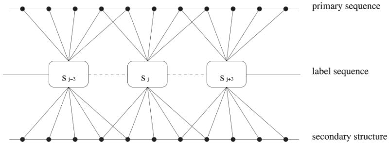
An example CRF model for protein conformation sampling. In this example, s_i (i.e., the label at position i) depends on the residues and secondary structure types at positions i−2, i−1, i, i+1, and i+2 and any nonlinear combinations of them. There is also interdependence between two adjacent labels. This CRF model can also be extended to incorporate long-range interdependence between two labels.

Model features

CRFSampler uses two different types of feature functions. At each position i, CRFSampler uses e(s_i−1,s_i) = [s_i−1 = h₁] [s_i = h₂] as its edge feature function. That is, currently, we only consider the first order dependence between labels. We are also investigating the second order dependence between labels. We use the following label feature functions to model the relationship among primary sequence, secondary structure, and backbone angles. Meanwhile, w is half of the window size.

1. ν_1,j(o,s_i) = [A_i+j = a] [s_i = h]. This feature set describes the interdependence between the label at position i and the residue at position i+j, where − w ≤ j ≤ w. A feature in this set is identified by a triple (a, h, j).

2. ν_2,j(o,s_i) = [X_i+j = x] [s_i = h]. This feature set describes the interdependence between the label at position i and the secondary structure type at position i + j, where −w ≤ j ≤ w. A feature in this set is identified by a triple (x, h, j).

3. ν_3,j(o,s_i) = [A_i+j = a] [X_i+j = x] [s_i = h]. This feature set describes the interdependence among the label at position i, the residue at position i + j, and the secondary structure type at position i + j where −w ≤ j ≤ w. A feature in this set represents a nonlinear combination of secondary structure and primary sequence and is identified by a quadruple (a, x, h, j).

In this article, we use a window size 9 (i.e., w = 4), which is slightly better than a window size 5 when predicted secondary structure information is used as input of CRFSampler (see Table I in Results section). In total there are more than ten thousand features in CRFSampler quantifying protein sequence-structure relationship.

Table I. F1-Values (%) of CRFSampler with Respect to Window Size.

Window size	a	b	c	d
1	10.01	10.02	15.30	17.34
5	14.08	17.50	19.65	20.49
9	14.76	18.58	19.81	20.89

F1-value is an even combination of precision (p) and recall (r) and defined as 2pr/(p + r). a, trained and tested using primary sequence; b, trained and tested using PSI-BLAST sequence profile; c, trained and tested using primary sequence and PSIPRED-predicted secondary structure; d, trained and tested using PSI-BLAST sequence profile and PSIPRED-predicted secondary structure confidence scores.

Extension to continuous-valued observations

We can also extend CRFSampler to make use of sequence profile and predicted secondary structure likelihood scores to improve sampling performance. In this case, for each protein, the observation is not two strings any more but consists of two matrices. One is the position-specific frequency matrix containing 20 × N entries (where N is the number of residues in a protein); each element in this matrix is the occurring frequency of one amino acid at a given position. The other matrix is the PSIPRED-predicted secondary structure likelihood matrix containing 3 × N elements; each element is the predicted likelihood of one secondary structure type at a specific position. To use this kind of continuous-valued observations, we extend label feature functions as follows. In defining ν_l,j(o, s_i) (l = 1,2,3), instead of assigning [A_i+j = a] to a binary value (i.e., 0 or 1), we assign [A_i+j = a] to the frequency of amino acid a appearing at position i+j. Similarly, we assign [X_i+j =x] to the PSIPRED-predicted likelihood of secondary type x at position i + j.

Conformation sampling algorithm

Sample one conformation for the whole protein

Given a CRF model and its parameters, we used a forward-backward sampling algorithm to generate protein conformations. The algorithm is an extension of the sampling algorithm described for the HMM model.¹⁷ The major difference is that our sampling algorithm needs to deal with many more sophisticated features and we also need to transform likelihood to probability in sampling. Let ν_l(i, h) denote a label feature function associated with position i and label h. For a given position i and a label h, we recursively define and calculate G(i, h) from N-terminal to C-terminal as follows.

$$\begin{array}{l}G(0,h)=\text{exp}\left(\sum _l{\lambda }_l{\upsilon }_l(0,h)\right)\hfill \\ G(i,h)=\text{exp}\left(\sum _l{\lambda }_l{\upsilon }_l(i,h)\right)\sum _h(G(i-1,\overline{h})\text{exp}({\lambda }_{\overline{h},h}))\hfill \end{array}$$

where λ_l is the trained parameter for the label feature ν_l(,) and λ_h̄,h is the trained parameter for the edge feature e(h̄, h). After G(N − 1, h) (N is the protein size) is calculated, we can sample a conformation from C-terminal to N-terminal. First, we sample the label h for the last position according to probability G(N − 1,h)/Σ_h G(N − 1, h). Then we sample the label h̄ for position i according to probability (G(i, h̄) exp(λ_h̄,h))/(Σ_h̄ G(i, h̄) exp(λ_h̄,h)), supposing that the sampled label at position i + 1 is h. Note that each label corresponds to a distribution of backbone angles. Based on the sampled labels, we can sample the two backbone angles for each position and build a backbone conformation for the protein.

Resample a small segment of the backbone conformation

Given a backbone conformation, we generate the next conformation by resampling a small segment of the protein. First, we randomly sample the starting position of the segment and its length. The length is uniformly sampled from 1 to 15. We resample the labels of the segment including positions i, i + 1, …, j, conditioned on the current labels at positions i − 1 and j + 1. Suppose that the labels at positions i − 1 and j + 1 are h₁ and h₂, respectively. We calculate Ḡ(k, h) (i ≤ k ≤ j) from position i to j as follows.

$$\begin{array}{l}\overline{G}(i,h)=\text{exp}\left(\sum {\lambda }_l{\nu }_l(i,h)\right)\text{exp}({\lambda }_{h1},h)\hfill \\ \overline{G}(k,h)=\text{exp}\left(\sum {\lambda }_l{\nu }_l(k,h)\right)\sum _{\overline{h}}(\overline{G}(k-1,\overline{h})\text{exp}({\lambda }_{\overline{h},h}))\hfill \end{array}$$

After calculating G(k, h) for all all the k between i and j, we can sample the labels for the segment from j to i. At position j−1, we sample a label h according to probability (Ḡ(j − 1, h) exp(λ_h,h2))/(Σ_h Ḡ(j − 1, h) exp((λ_h,h2)). For any position k (i ≤ k ≤ j − 1), we sample a label h according to probability (Ḡ(k, h)exp(λ_h,h̄))/(Σ_hḠ(k,h) exp(λ_h,h̄)), supposing h̄ is the sampled label at position k+1. After resampling the labels of this segment, we can resample the angles of this segment and then rebuild the backbone conformation.

Folding simulation

Since the focus of this artcle is the protein conformation sampling algorithm, we use only compactness and self-avoiding constraints to drive conformation search during the folding simulation process. We start with sampling the whole backbone conformation of a given protein and then optimize its conformation by minimizing the radius of gyration. Given a conformation, we generate its next potential conformation by resampling the local conformation of a small segment. If this potential conformation has no serious steric clashes among atoms, then we compare its radius with that of current conformation. If this potential conformation has a smaller radius, then we accept this conformation, otherwise reject it. This process is terminated if no better conformations can be found within 1000 consecutive resamplings. There is a steric clash if the distance between two C_α atoms is less than 4 Å.

Results

Data set

We tested CRFSampler on the following proteins: 1FC2, 1ENH, 2GB1, 2CRO, 1CTF, 4ICB, 1AA2, 1BEO, 1DKT, 1FCA, 1FGP, 1JER, 1NKL, 1PGB, 1SRO, 1TRL, T0052 (PDB code: 2EZM), T0056 (1JWE), T0059 (1D3B), T0061 (1BG8), T0064 (1B0N), and T0074 (1EH2). Meanwhile, the first six have been studied in Refs. 2 and ¹⁷; and the last 18 in Ref. 32; the last six proteins are also CASP3 targets. We obtained a set of non-redundant protein structures using the PISCES server³³ as our training data. Each protein in this set has resolution at least 2.0 Å, R factor no bigger than 0.25 and at least 30 residues. Any two proteins in this set share no more than 30% sequence identity. To avoid overlap between the training data and the test proteins, we removed the following proteins from our training data:(1) the proteins sharing at least 25% sequence identity with our test proteins; (2) the proteins in the same fold class as our test proteins according to the SCOP classification³⁴; and (3) the proteins having a TM-score ≥ 0.5 with our test proteins in case some recently released proteins do not have a SCOP ID. According to Ref. 35, if the TM-score of two protein structures is smaller than 0.5, then a threading program such as PROSPECTOR_3³⁶ cannot identify their similarity relationship with high confidence.

Label assignment and distribution parameters

To train CRFSampler, we also need to assign a label to each position in a protein. In this article, we only tested our algorithm on the (θ, τ) representation of a protein backbone conformation. There can be various methods to assign a label to a protein position. For example, we can cluster all the (θ, τ) angles into dozens of groups; each group corresponds to a label. Here, we just simply use the five-residue fragment libraries developed by Kolodny et al.³⁷ since these libraries have already been carefully designed. The library containing 100 five-residue fragments is used as the set of hidden labels; each label corresponds to a cluster in the fragment library. We calculated the (θ, τ) distribution for each cluster from the training proteins using the KentEstimator program enclosed in Mocapy.¹⁷ Only the angles of the middle residue in a fragment are used to calculate the angle distribution parameters. We also tested other four-residue and five-residue fragment libraries developed by Kolodny et al. and it turns out that the five-residue fragment library with 100 clusters yields the best performance.

Parameter tuning

We randomly divided the training proteins into five sets of same size and then used them for five-fold cross validation. We trained CRFSampler using several different regularization factors [i.e., σ² in Eq. (8)]: 50, 100, 200, 400, and 800 and choose the one with the best F1-value. F1-value is a widely used measurement of the prediction capability of a machine learning model in the machine learning community. F1-value is an even combination of precision (p) and recall (r) and defined as 2pr/(p + r). The higher the F1-value is, the better. When both PSI-BLAST sequence profile and PSIPRED-predicted secondary structure likelihood scores are used and a window size 9 is used to define the model features, the average F1-values for regularization factors 50, 100, 200, 400, and 800 are 20.82%, 20.89%, 20.83%, 20.71%, and 20.56%, respectively. In fact, there is no big difference among these regularization factors in terms of F1-value. However, we prefer to choose a small regularization factor 100 to control the model complexity. The regularization factor is the only parameter that we need to tune manually. All the other model parameters (i.e., weights for features) can be estimated automatically in training.

In addition, we also tested the performance of our algorithm with respect to window size in defining model features. As shown in Table 1, our experimental results indicate that when 100 labels are used in CRFSampler, a window size 5 can yield a much higher F1-value than a window size 1. Increasing the window size to 9 can improve the F1-value, but the improvement is small when PSIPRED-predicted secondary structure is used in CRFSampler. This may be because the predicted secondary structure also contains partial information of neighbor residues. In our remaining experiments, we used window size 9 to define model features for CRFSampler.

Comparison with the HMM model¹⁷

It is not easy to fairly compare two protein conformation sampling algorithms. Many ab initio folding programs use a sophisticated energy function to drive conformation search and it is hard to evaluate performance of their conformation sampling algorithms alone, without considering their energy functions. The focus of this paper lies in only protein conformation sampling algorithm. To evaluate the sampling algorithm, we drive conformation search by minimizing the radius of gyration instead of a well-designed energy function. In this paper, we compare CRFSampler mainly with the HMM method described in Ref. 17, which is also a protein conformation sampling algorithm and drives conformation search by minimizing the radius instead of an energy function. The major difference between CRFSampler and the HMM model is that the former generates conformations using a CRF model while the latter uses an HMM model. We tested CRFSampler on six proteins studied in Ref. 17 and compared the quality of the decoys generated by CRFSampler with those by the HMM model.¹⁷

Since for most proteins without known structures, we cannot obtain their true secondary structures, here we compare the HMM model and CRFSampler using only PSIPRED-predicted secondary structure and sequence information as their inputs. As shown in Table II, when only sequence information used, CRFSampler can generate decoys with much higher quality than the HMM model. The only exception is that the HMM model has a comparable performance with CRFSampler on 1ENH when only primary sequence is used. When only primary sequence is used, the number of good decoys (RMSD ≤ 6 Å) generated by CRFSampler is 2 ∼ 4 times that by the HMM model. This difference comes from the fact that in sampling the angles at one position, CRFsampler can directly take into consideration the effects of its neighbor residues. When predicted secondary structure is used, as shown in Table III, CRFSampler is much better than the HMM model in generating good decoys and the best decoys. Among the six test proteins, CRFSampler is slightly worse than the HMM model on the Calbidin protein (PDB code: 4ICB) when predicted secondary structure type is used. For the other five proteins, CRFSampler can generate many more good decoys. CRFSampler can also generate the best decoys with much smaller RMSDs, although only 20,000 decoys are generated by CRFSampler for each test protein while 100,000 decoys by the HMM model for each test protein. By using PSI-BLAST sequence profile and predicted secondary structure likelihood scores as input, CRFSampler can achieve overall performance better than using primary sequence and predicted secondary structure types. This indicates the importance of using continuous-valued observations in a conformation sampling algorithm. By contrast, it is not easy for the HMM model to incorporate these kind of continuous-valued observations as input. Figure 2 visualizes the native structures and the best decoys (generated by CRFSampler) of the six test proteins.

Table II. Decoy Quality Comparison Between the HMM Model¹⁷ and CRFSampler.

Test proteins			HMMa		CRFSamplerb		CRFSamplerc
Name, PDB code	L	α,β	Good (%)	Best (Å)	Good (%)	Best (Å)	Good (%)	Best (Å)
Protein A, 1FC2	43	2,0	9.59	2.7	20.9	2.08	24.8	2.09
Homeodomain, 1ENH	54	2,0	6.60	2.5	6.23	2.68	14.0	1.98
Protein G, 2GB1	56	1,4	0.04	4.9	0.16	4.67	10.1	3.36
Cro repressor, 2CRO	65	5,0	0.46	3.9	1.94	4.05	13.3	2.37
Protein L7/L12, 1CTF	68	3,1	0.01	5.4	0.04	4.94	0.15	4.49
Calbidin, 4ICB	76	4,0	0.09	4.3	0.17	4.57	0.42	4.72

Only sequence information is used in both training and testing. In total, 100,000 decoys are generated by the HMM model.

Columns 1–3 list name and PDB code, length and number of α-helices and β-strands of the test proteins. Columns “Good” and “Best” list the percentage of good decoys (with RMSD ≤ 6 Å) and the RMSD of the best decoy, respectively.

^aTrained and tested using primary sequence and the results are taken from Ref. 17.

^bTrained and tested using primary sequence and 40,000 decoys are generated.

^cTrained and tested using PSI-BLAST sequence profile. Only 20,000 decoys are generated.

Table III. Decoy Quality Comparison Between the HMM Model¹⁷ and CRFSampler.

Test proteins			HMMa		CRFSamplerb		CRFSamplerc
Name, PDB code	L	α,β	Good (%)	Best (Å)	Good (%)	Best (Å)	Good (%)	Best (Å)
Protein A, 1FC2	43	2,0	17.1	2.6	26.8	2.13	49.1	1.94
Homeodomain, 1ENH	54	2,0	12.2	3.8	16.7	2.29	22.4	2.32
Protein G, 2GB1	56	1,4	0.0	5.9	26.4	3.05	23.3	2.91
Cro repressor, 2CRO	65	5,0	1.1	4.1	18.3	2.76	16.8	2.79
Protein L7/L12, 1CTF	68	3,1	0.35	4.1	3.0	4.04	2.4	3.70
Calbidin, 4ICB	76	4,0	0.38	4.5	0.24	4.45	0.51	4.63

Both sequence and secondary structure information are used. In total, 100,000 decoys are generated by the HMM model while only 20,000 decoys by each CRFSampler.

Columns 1–3 list name and PDB code, length and number of α-helices and β-strands of the test proteins. Column “Good” lists the percentage of good decoys (with RMSD ≤ 6 Å). Column “Best” lists the RMSD of the best decoy for each test protein.

^aTrained using true secondary structure and primary sequence while tested using predicted secondary structure (by PSIPRED³⁸) and primary sequence and the results are taken from Ref. 17.

^bTrained and tested using predicted secondary structure (by PSIPRED) and primary sequence.

^cTrained and tested using predicted secondary structure likelihood scores (by PSIPRED) and PSI-BLAST sequence profile.

Figure 2. Native structures (in orange) and the best decoys of 1FC2, 1ENH, 2GB1, 2CRO, 1CTF, and 4ICB.

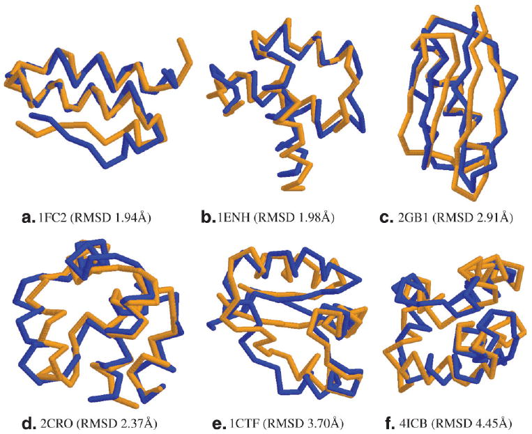
Table IV lists the percentage of correct secondary structure (i.e., Q3-value) of all the good decoys generated by CRFSampler for each test protein. A software P-SEA³⁹ is used to calculate the secondary structure of a decoy. As shown in this table, even with primary sequence only, CRFSampler can generate decoys with pretty good Q3-values, better than the HMM model (see Table II in Ref. 17). This confirms that CRFSampler can capture well the relationship between a sequence stretch and its local conformation.

Table IV. Secondary Structure Content of Good Decoys.

	CRFSamplera
Protein	Q3	H	E	C
1FC2	66.5	61.3	1.8	36.9
1ENH	79.3	69.2	2.9	27.9
2GB1	65.2	29.5	24.9	45.7
2CRO	80.0	71.6	2.3	26.2
1CTF	67.1	50.3	9.5	40.1
4ICB	65.0	59.6	2.9	37.5
	CRFSamplerb
1FC2	75.2	49.4	1.9	48.7
1ENH	79.2	64.9	7.1	28.0
2GB1	61.0	24.1	27.6	48.2
2CRO	85.2	66.0	1.8	32.2
1CTF	62.6	41.8	19.7	38.5
4ICB	66.6	59.0	5.0	36.0
	CRFSamplerc
1FC2	85.5	55.1	1.0	43.9
1ENH	86.0	64.3	2.9	32.8
2GB1	72.0	24.8	32.9	42.3
2CRO	87.1	69.3	1.5	29.1
1CTF	77.5	56.9	10.6	32.5
4ICB	65.7	62.0	3.81	34.2
	CRFSamplerd
1FC2	80.7	61.9	0.2	37.9
1ENH	85.1	67.3	3.0	29.7
2GB1	71.5	25.9	29.7	44.4
2CRO	85.9	67.5	1.6	31.0
1CTF	77.2	59.5	8.6	31.9
4ICB	67.1	63.1	2.5	34.4

^aPercentage correct secondary structure (Q3-value) and secondary structure content of good decoys (RMSD ≤ 6 Å) generated using primary sequence.

^bQ3-value and secondary structure content of good decoys generated using PSI-BLAST sequence profile.

^cQ3-value and secondary structure content of good decoys generated using primary sequence and PSIPRED-predicted predicted secondary structure.

^dQ3-value and secondary structure content of good decoys generated using PSI-BLAST sequence profile and PSIPRED-predicted secondary structure likelihood scores.

Comparison with Xia et al.³²

In Ref. 32, Xia et al. have developed a hierarchical method to generate decoys. This method first exhaustively enumerates all the possible conformations on a lattice model for a given protein sequence and then builds conformations with increasing detail. At each step, this method chooses a good subset of conformations using hydrophobic compactness constraint and empirical energy functions such as RAPDF⁴⁰ and Shell⁴¹ and finally generate 10,000 or 40,000 decoys for a protein sequence. Table V lists the RMSD ranges of all the decoys generated by this method and CRFSampler for 18 test proteins. As shown in this table, CRFSampler can generate decoys with smaller RMSD on all the test proteins with less than 100 residues. CRFSampler is significantly better than this hierarchical method on 1CTF, 1NKL, 1PGB, 1SRO, 1TRL-A, T0052, T0059 and T0074 in terms of the best decoys. For those test proteins with more than 100 residues, CRFSampler is worse than the method of Xia et al. on two proteins (1AA2 and T0056) and better one on protein (T0064), and has comparable performance on 1JER. This may indicate that we need to improve CRFSampler further to search conformation space more effectively for a protein with more than 100 residues. We also used the Wilcoxon signed-rank test,⁴² a nonparametric alternative to the paired Student's t-test, to calculate the significance level at which CRFSampler is better than the method of Xia et al. Since we only had the RMSD ranges of the decoys generated by Xia et al., we only considered the best decoys in calculating the statistical test. For the first 12 proteins in Table V, we used the best decoys in a set of randomly chosen CRFSampler 10,000 decoys since Xia et al. only generated 10,000 final decoys for these proteins. For the last six proteins, we used their best decoys listed in Table V. When the absolute RMSD difference between the best decoys is used to calculate the statistical test, CRFSampler is better than the method of Xia et al. at significance level 0.01.^¶ When the relative RMSD difference is used, CRFSampler is better than the method of Xia et al. at significance level 0.005. Finally, CRFSampler tends to generate decoys with larger RMSD variance because CRFSampler does not use any empirical energy functions to filter those bad conformations.

Table V. Decoy Quality Comparison Between Xia et al.³² and CRFSampler.

Test proteins			Xia et al.	CRFSampler
PDB code	L	Class	All RMSD range	All RMSD range
1aa2	108	α	6.18–15.28	7.34–17.06
1beo	98	α	6.96–15.94	6.41–16.95
1ctf	68	α + β	5.45–13.54	3.70–13.37
1dktA	72	β	6.68–14.79	6.14–15.51
1fca	55	β	5.09–12.06	4.98–12.90
1fgp	67	β	7.80–14.40	7.39–15.20
1jer	110	β	9.55–17.53	9.63–19.64
1nkl	78	α	5.26–14.23	3.63–13.76
1pgb	56	α + β	5.60–13.30	3.15–12.75
1sro	76	β	7.30–15.42	6.22–15.70
1trlA	62	α	5.30–13.16	3.53–12.43
4icb	76	α	4.74–13.28	4.63–13.93
T0052	98	β	10.6–16.3	7.58–19.17
T0056	114	α	6.2–17.8	7.77–18.17
T0059	71	β	7.4–15.7	6.29–15.54
T0061	76	α	6.0–14.0	5.35–14.84
T0064	103	α	8.0–18.8	7.23–18.85
T0074	98	α	6.3–16.5	4.85–15.72

CRFSampler generated 20,000 decoys for each test protein using PSI-BLAST sequence profile and predicted secondary structure likelihood scores. Xia et al.³² conducted a complete enumeration on a lattice model for each test protein and then generated 10,000 decoys for each of the first 12 proteins and 40,000 decoys for each of the six CASP3 targets, respectively, using predicted secondary structure and empirical energy functions as filters.

We also calculated the secondary structure content of all the decoys using P-SEA³⁹ and compared CRFSampler with PSIPRED³⁸ in terms of Q3-value. As shown in Table VI, CRFSampler can generate decoys with reasonable level of secondary structure accuracy. The average Q3-value of all the decoys generated by CRFSampler is 70.3% while the average PSIPRED Q3-value of these test proteins is 74.4%. The Wilcoxon signed-rank test indicates that in terms of Q3-value, CRFSampler is worse than PSIPRED at significance level 0.025.

Table VI. Percentage Correct Secondary Structure (Q3-value) and Secondary Structure Content of all the Decoys Generated by CRFSampler, Compared with PSIPRED Predictions.

Test proteins			CRFSampler				PSIPRED
PDB code	L	Class	Q3	H	E	C	Q3	H	E	C
1aa2	108	α	78.5	53.9	5.4	40.7	88.0	56.5	1.9	41.7
1beo	98	α	68.4	51.3	9.9	38.7	65.3	42.9	6.1	51.0
1ctf	68	α + β	76.9	59.8	8.6	31.6	77.9	55.9	13.2	30.9
1dktA	72	β	53.7	16.3	28.4	55.3	50	15.3	30.6	54.2
1fca	55	β	71.9	4.7	16.8	78.5	83.6	0.0	16.4	83.6
1fgp	67	β	57.3	4.5	28.5	66.9	64.3	0.0	35.7	64.2
1jer	110	β	63.2	14.1	34.7	51.2	74.3	8.3	37.6	54.1
1nkl	78	α	87.7	75.3	0.4	24.3	92.3	73.1	0.0	26.9
1pgb	56	α + β	67.3	25.6	27.8	46.7	80.4	21.4	50	28.6
1sro	76	β	59.2	7.7	28.8	63.5	56.6	10.5	43.4	46.1
1trlA	62	α	80.9	70.0	0.4	29.6	83.9	67.7	0.0	32.3
4icb	76	α	67.2	61.8	3.5	34.8	67.1	60.5	2.6	36.8
T0052	98	β	54.1	6.0	36.1	57.9	54.5	8.9	42.6	48.5
T0056	114	α	83.3	71.2	1.4	27.5	81.6	74.6	0.0	25.4
T0059	71	β	64.9	10.4	41.3	48.3	72.2	8.3	52.8	38.9
T0061	76	α	59.9	42.0	13.7	44.3	71.1	40.8	14.5	44.7
T0064	103	α	87.2	66.2	2.7	31.0	94.2	67.0	0.0	33.0
T0074	98	α	84.9	53.6	3.2	43.2	83.2	55.8	0.0	44.2

The average Q3-value of all the decoys is 70.3% while the average PSIPRED Q3-value is 74.4%. CRFSampler is worse than PSIPRED at significance level 0.025.

Comparison with Rosetta

Here, we compare CRFSampler with the well-known fragment-assembly-based program Rosetta.² Rosetta uses multiple sequence alignment information to choose 25 fragments for each sequence segment of nine residues and then assembles them into decoys using a time-consuming simulated annealing procedure. Rosetta drives conformation search using a well-developed energy function and generates a few hundred decoys, while CRFSampler generates 20,000 decoys without using any energy function. Although this comparison is interesting, we want to point out it is also unfair to both CRFSampler and Rosetta. On one hand, CRFSampler does not use an energy function to drive conformation search. On the other hand, the result for Rosetta is taken from a article published in 1997, which may not be the performance of the state-of-the-art Rosetta. As indicated in Table VII, by quickly generating a large number of decoys, CRFSampler can obtain decoys with much smaller RMSD than Rosetta. However, it is also not surprising that Rosetta can generate higher percentage of good decoys for five out of six test proteins by using a time-consuming energy minimization procedure.

Table VII. Decoy Quality Comparison Between ROSETTA² and CRFSampler.

Test proteins			ROSETTAa		CRFSamplerb		CRFSamplerc
Name, PDB code	L	α, β	Good (%)	Best (Å)	Good (%)	Best (Å)	Good (%)	Best (Å)
Protein A, 1FC2	43	2,0	95	3.3	20.9	2.08	24.8	2.09
Homeodomain, 1ENH	54	2,0	47	2.7	6.23	2.68	14.0	1.98
Protein G, 2GB1	56	1,4	0.0	6.3	0.16	4.67	10.1	3.36
Cro repressor, 2CRO	65	5,0	18.0	4.2	1.94	4.05	13.3	2.37
Protein L7/L12, 1CTF	68	3,1	6.0	5.3	0.04	4.94	0.15	4.49
Calbidin, 4ICB	76	4,0	17	4.7	0.17	4.57	0.42	4.72

Only sequence information is used in both training and testing. ROSETTA generates a few hundred decoys using energy function optimization while CRFSampler generates 20,000 decoys by minimizing radius of gyration.

Columns 1-3 list name and PDB code, length and number of α-helices and β-strands of the test proteins. Columns “Good” and “Best” list the percentage of good decoys (with RMSD ≤ 6Å) and the RMSD of the best decoy, respectively.

^aMultiple sequence alignment information is used and the results are taken from Ref. 2.

^bTrained and tested using primary sequence.

^cTrained and tested using PSI-BLAST sequence profile.

Computational efficiency

Although we have not optimized the C++ code of CRFSampler, CRFSampler can quickly generate a decoy within seconds for a test protein. Table VIII the approximate running time in minutes spent by CRFSampler generating 100 decoys for each test protein, on a single 2.2 GHz CPU. As indicated in this table, CRFSampler can generate decoys for these test proteins very quickly. It takes CRFSampler approximately 1 h to generate 100 decoys for protein G (2GB1) and no more than ten minutes for 1FC2. It does not increase the running time of CRFSampler by using more information as input such as PSI-BLAST sequence profile and secondary structure likelihood scores. Instead, using them tend to reduce the running time of CRFSampler, maybe because of the reduction in the entropy of conformation search space.

Table VIII. Approximate Running Time in Minutes Spent by CRFSampler in Generating 100 Decoys.

	1FC2	1ENH	2GB1	2CRO	1CTF	4ICB
a	7.0	13.0	45.5	29.5	46.0	37.5
b	8.0	12.0	63.0	14.5	78.0	43.5
c	6.0	7.5	67.5	7.5	16.0	29.5
d	4.0	8.0	56.0	7.0	13.0	27.5

a, Trained and tested using primary sequence; b, Trained and tested using PSI-BLAST sequence profile; c, Trained and tested using PSIPRED-predicted secondary structure and primary sequence; d, Trained and tested using PSIPRED-predicted secondary structure confidence scores and PSI-BLAST sequence profile.

Discussion

This article presented an extensible and fully automatic framework CRFSampler that can be used to effectively sample conformations of a protein from its sequence information and predicted secondary structure. CRFSampler uses thousands of parameters to quantify the relationship among backbone angles, primary sequence and secondary structure without worrying about risk of overfitting. Experimental results demonstrate that CRFSampler is more effective in sampling conformations than the HMM model.¹⁷ CRFSampler is quite flexible. Using CRFSampler, the user only needs to choose a set of appropriate features describing the relationship between protein sequence and structure. CRFSampler can take care of the remaining tasks such as parameter estimation and conformation sampling.

Currently, CRFSampler only takes into consideration the dependency between two adjacent positions. Our future work is to incorporate the interdependency among more residues into CRFSampler so that CRFSampler can explore conformation space of a medium-sized protein (≥ 100 residues) more effectively. For example, given the labels at positions i and i + 1, there are on average only 10 possible labels at position i + 2. Given the labels at positions i and i + 2, there are on average only 16 possible labels at position i + 4. If this kind of constraint information is incorporated into CRFSampler, it can greatly reduce the entropy of conformation search space and is very likely to scale CRFSampler up to proteins with more than 100 residues. Another way to reduce the entropy of the conformation search space is to treat a label as a distribution of a short structural fragment. We can develop a discriminative approach to predicting the occurring probability of one fragment at a given position and the probability of connecting one fragment to its next one. Our experimental results indicate that using predicted secondary structure, the sampling performance of CRFSampler can be improved dramatically, compared to using PSI-BLAST sequence profile only. We can also incorporate other predicted information such as solvent accessibility and contact capacity (i.e., the number of contacts for a residue) into CRFSampler, which may improve sampling performance. In addition, if some distance restraints can be obtained from NMR data or comparative modeling, then it is also possible to extend CRFSampler to incorporate long-range interdependency. CRFSampler can also be extended to make use of other NMR data sources such as chemical shifts⁴³ and residue dipolar coupling (RDC) data.⁴⁴

In this paper, we drive the conformation optimization by minimizing the radius of gyration. Our next step is to couple CRFSampler with a good energy function such as DOPE⁴⁵ and DFIRE,⁴⁶ to do real protein structure prediction. The decoys generated by CRFSampler can also be used to benchmark energy functions since CRFSampler does not employ any energy function to generate these decoys and thus no energy-bias is introduced into these decoys.

References

- 1.Moult J. A decade of casp: progress, bottlenecks and prognosis in protein structure prediction. Cur Opin Struct Biol. 2005;15:285–289. doi: 10.1016/j.sbi.2005.05.011. [DOI] [PubMed] [Google Scholar]
- 2.Simons KT, Kooperberg C, Huang E, Baker D. Assembly of protein tertiary structures from fragments with similar local sequences using simulated annealing and bayesian scoring functions. J Mol Biol. 1997;268:209–225. doi: 10.1006/jmbi.1997.0959. [DOI] [PubMed] [Google Scholar]
- 3.Moult J, Fidelis K, Zemla A, Hubbard T. Critical assessment of methods of protein structure prediction (casp)-round v. Proteins. 2003;53(S6):334–339. doi: 10.1002/prot.10556. [DOI] [PubMed] [Google Scholar]
- 4.Moult J, Fidelis K, Rost B, Hubbard T, Tramontano A. Critical assessment of methods of protein structure prediction (casp)-round 6. Proteins. 2005;61 7:3–7. doi: 10.1002/prot.20716. [DOI] [PubMed] [Google Scholar]
- 5.Zhang Y, Skolnick J. The protein structure prediction problem could be solved using the current pdb library. Proc Nat Acad Sci USA. 2005;102:1029–1034. doi: 10.1073/pnas.0407152101. [DOI] [PMC free article] [PubMed] [Google Scholar]
- 6.Jones TA, Thirup S. Using known substructures in protein model building and crystallography. EMBO J. 1986;5:819–823. doi: 10.1002/j.1460-2075.1986.tb04287.x. [DOI] [PMC free article] [PubMed] [Google Scholar]
- 7.Claessens M, van Cutsem E, Lasters I, Wodak S. Modelling the polypeptide backbone with ‘spare parts’ from known protein structures. Protein Eng. 1989;2:335–345. doi: 10.1093/protein/2.5.335. [DOI] [PubMed] [Google Scholar]
- 8.Unger R, Harel D, Wherland S, Sussman JL. A 3D building blocks approach to analyzing and predicting structure of proteins. Proteins. 1989;5:355–373. doi: 10.1002/prot.340050410. [DOI] [PubMed] [Google Scholar]
- 9.Simon I, Glasser L, Scheraga HA. Calculation of protein conformation as an assembly of stable overlapping segments: application to bovine pancreatic trypsin inhibitor. Proc Nat Acad Sci. 1991;88:3661–3665. doi: 10.1073/pnas.88.9.3661. [DOI] [PMC free article] [PubMed] [Google Scholar]
- 10.Levitt M. Accurate modeling of protein conformation by automatic segment matching. J Mol Biol. 1992;226:507–533. doi: 10.1016/0022-2836(92)90964-l. [DOI] [PubMed] [Google Scholar]
- 11.Sippl M. Recognition of errors in three-dimensional structures of proteins. Proteins. 1993;17:355–362. doi: 10.1002/prot.340170404. [DOI] [PubMed] [Google Scholar]
- 12.Wendoloski JJ, Salemme FR. Probit: a statistical approach to modeling proteins from partial coordinate data using substructure libraries. J Mol Graph. 1992;10:124–126. doi: 10.1016/0263-7855(92)80066-m. [DOI] [PubMed] [Google Scholar]
- 13.Bowie JU, Eisenberg D. An evolutionary approach to folding small α-helical proteins that uses sequence information and an empirical guiding fitness function. Proc Nat Acad Sci USA. 1994;91:4436–4440. doi: 10.1073/pnas.91.10.4436. [DOI] [PMC free article] [PubMed] [Google Scholar]
- 14.Bystroff C, Thorsson V, Baker D. HMMSTR: a hidden markov model for local sequence-structure correlations in proteins. J Mol Biol. 2000;301:173–190. doi: 10.1006/jmbi.2000.3837. [DOI] [PubMed] [Google Scholar]
- 15.Gong H, Fleming PJ, Rose GD. Building native protein conformation from highly approximate backbone torsion angles. Proc Nat Acad Sci USA. 2005;102:16227–16232. doi: 10.1073/pnas.0508415102. [DOI] [PMC free article] [PubMed] [Google Scholar]
- 16.Colubri A, Jha AK, Shen MY, Sali A, Berry RS, Sosnick TR, Freed KF. Minimalist representations and the importance of nearest neighbor effects in protein folding simulations. J Mol Biol. 2006;363:835–857. doi: 10.1016/j.jmb.2006.08.035. [DOI] [PubMed] [Google Scholar]
- 17.Hamelryck T, Kent JTT, Krogh A. Sampling realistic protein conformations using local structural bias. PLoS Comput Biol. 2006;2:e131. doi: 10.1371/journal.pcbi.0020131. [DOI] [PMC free article] [PubMed] [Google Scholar]
- 18.Kent JT. The fisher-bingham distribution on the sphere. J R Stat Soc. 1982;44:71–80. [Google Scholar]
- 19.Mardia KV, Taylor CC, Subramaniam GK. Protein bioinformatics and mixtures of bivariate von mises distributions for angular data. Biometrics. 2007;63:505–512. doi: 10.1111/j.1541-0420.2006.00682.x. [DOI] [PubMed] [Google Scholar]
- 20.Singh H, Hnizdo V, Demchuk E. Probabilistic model for two dependent circular variables. Biometrika. 2002;89:719–723. [Google Scholar]
- 21.Tuffery V, Derreumaux P. Dependency between consecutive local conformations helps assemble protein structures from secondary structures using go potential and greedy algorithm. Proteins. 2005;61:732–740. doi: 10.1002/prot.20698. [DOI] [PubMed] [Google Scholar]
- 22.Jha AK, Colubri A, Zaman MH, Koide S, Sosnick TR, Freed KF. Helix sheet, and polyproline ii frequencies and strong nearest neighbor effects in a restricted coil library. Biochemistry. 2005;44:9691–9702. doi: 10.1021/bi0474822. [DOI] [PubMed] [Google Scholar]
- 23.Ng A, Jordan M. On discriminative vs. generative classifiers: a comparison of logistic regressior and naive bayes. In: Dietterich T, Becker S, Ghahramani Z, editors. Advances neural information processing systems (NIPS) Cambridge, MA: MIT Press; 2002. [Google Scholar]
- 24.Lafferty J, Mccallum A, Pereira F. Conditional random fields: probabilistic models for segmenting and labeling sequence data. Proceedings of the 18th International Conference on Machine Learning; San Francisco, CA. 2001. pp. 282–289. [Google Scholar]
- 25.Sha F, Pereira F. Shallow parsing with conditional random fields. NAACL '03: Proceedings of the 2003 Conference of the North American Chapter of the Association for Computational Linguistics on Human Language Technology; Morristown, NJ, USA. 2003. pp. 134–141. [Google Scholar]
- 26.Levitt M. A simplified representation of protein conformations for rapid simulation of protein folding. J Mol Biol. 1976;104(1):59–107. doi: 10.1016/0022-2836(76)90004-8. [DOI] [PubMed] [Google Scholar]
- 27.Holm L, Sander C. Database algorithm for generating protein backbone and side-chain coordinates from a c alpha trace application to model building and detection of co-ordinate errors. J Mol Biol. 1991;218:183–194. doi: 10.1016/0022-2836(91)90883-8. [DOI] [PubMed] [Google Scholar]
- 28.Gront D, Kmiecik S, Kolinski A. Backbone building from quadrilaterals: a fast and accurate algorithm for protein backbone reconstruction from alpha carbon coordinates. J Comput Chem. 2007;28:1593–1597. doi: 10.1002/jcc.20624. [DOI] [PubMed] [Google Scholar]
- 29.Maupetit J, Gautier R, Tuffry P. Sabbac: online structural alphabet-based protein backbone reconstruction from carbon trace. Nucleic Acids Res. 2006;34(Web Server issue):W147–W151. doi: 10.1093/nar/gkl289. [DOI] [PMC free article] [PubMed] [Google Scholar]
- 30.Vapnik VN. Statistical learning theory. Wiley-Interscience; 1998. [Google Scholar]
- 31.Liu DC, Nocedal J. On the limited memory method for large scale optimization. Math Program B. 1989;45:503–528. [Google Scholar]
- 32.Xia Y, Huang ES, Levitt M, Samudrala R. Ab initio construction of protein tertiary structures using a hierarchical approach. J Mol Biol. 2000;300:171–185. doi: 10.1006/jmbi.2000.3835. [DOI] [PubMed] [Google Scholar]
- 33.Wang G, Dunbrack RL. Pisces: a protein sequence culling server. Bioinformatics. 2003;19:1589–1591. doi: 10.1093/bioinformatics/btg224. [DOI] [PubMed] [Google Scholar]
- 34.Murzin AG, Brenner SE, Hubbard T, Chothia C. Scop: a structural classification of proteins database for the investigation of sequences and structures. J Mol Biol. 1995;247:536–540. doi: 10.1006/jmbi.1995.0159. [DOI] [PubMed] [Google Scholar]
- 35.Zhang Y, Skolnick J. Tm-align: a protein structure alignment algorithm based on the tm-score. Nucleic Acids Res. 2005;33:2302–2309. doi: 10.1093/nar/gki524. [DOI] [PMC free article] [PubMed] [Google Scholar]
- 36.Skolnick J, Kihara D, Zhang Y. Development and large scale benchmark testing of the prospector_3 threading algorithm. Proteins. 2004;56:502–518. doi: 10.1002/prot.20106. [DOI] [PubMed] [Google Scholar]
- 37.Kolodny R, Koehl P, Guibas L, Levitt M. Small libraries of protein fragments model native protein structures accurately. J Mol Biol. 2002;323:297–307. doi: 10.1016/s0022-2836(02)00942-7. [DOI] [PubMed] [Google Scholar]
- 38.Mcguffin LJ, Bryson K, Jones DT. The psipred protein structure prediction server. Bioinformatics. 2000;16:404–405. doi: 10.1093/bioinformatics/16.4.404. [DOI] [PubMed] [Google Scholar]
- 39.Labesse G, Colloc'h N, Pothier J, Mornon JP. P-SEA: a new efficient assignment of secondary structure from c alpha trace of proteins. Comput Appl Biosci. 1997;13:291–295. doi: 10.1093/bioinformatics/13.3.291. [DOI] [PubMed] [Google Scholar]
- 40.Samudrala R, Moult J. An all-atom distance-dependent conditional probability discriminatory function for protein structure prediction. J Mol Biol. 1998;275:895–916. doi: 10.1006/jmbi.1997.1479. [DOI] [PubMed] [Google Scholar]
- 41.Park BH, Huang ES, Levitt M. Factors affecting the ability of energy functions to discriminate correct from incorrect folds. J Mol Biol. 1997;266:831–846. doi: 10.1006/jmbi.1996.0809. [DOI] [PubMed] [Google Scholar]
- 42.Wilcoxon F. Individual comparisons by ranking methods. Biometrics. 1945;1:80–83. [Google Scholar]
- 43.Neal S, Berjanskii M, Zhang H, Wishart DS. Accurate prediction of protein torsion angles using chemical shifts and sequence homology. Magn Resonan Chem. 2006;44(S1):S158–S167. doi: 10.1002/mrc.1832. [DOI] [PubMed] [Google Scholar]
- 44.Meiler J, Peti W, Griesinger C. Dipocoup: a versatile program for 3d-structure homology comparison based on residual dipolar couplings and pseudocontact shifts. J Biomol NMR. 2000;17:283–294. doi: 10.1023/a:1008362931964. [DOI] [PubMed] [Google Scholar]
- 45.Shen MY, Sali A. Statistical potential for assessment and prediction of protein structures. Protein Sci. 2006;15:2507–2524. doi: 10.1110/ps.062416606. [DOI] [PMC free article] [PubMed] [Google Scholar]
- 46.Zhang C, Liu S, Zhou H, Zhou Y. An accurate, residue-level, pair potential of mean force for folding and binding based on the distance-scaled, ideal-gas reference state. Protein Sci. 2004;13:400–411. doi: 10.1110/ps.03348304. [DOI] [PMC free article] [PubMed] [Google Scholar]