Detecting Consistent Common Lines in Cryo-EM by Voting

Abstract

The single-particle reconstruction problem of electron cryo-microscopy (cryo-EM) is to find the three-dimensional structure of a macromolecule given its two-dimensional noisy projection images at unknown random directions. Ab initio estimates of the 3D structure are often obtained by the “Angular Reconstitution” method, in which a coordinate system is established from three projections, and the orientation of the particle giving rise to each image is deduced from common lines among the images. However, a reliable detection of common lines is difficult due to the low signal-to-noise ratio of the images. In this paper we describe a global self-correcting voting procedure in which all projection images participate to decide the identity of the consistent common lines. The algorithm determines which common line pairs were detected correctly and which are spurious. We show that the voting procedure succeeds at relatively low detection rates and that its performance improves as the number of projection images increases. We demonstrate the algorithm for both simulative and experimental images of the 50S ribosomal subunit.

1. Introduction

“Three-dimensional electron microscopy” [Frank, 2006] is the name commonly given to methods in which the 3D structures of macromolecular complexes are obtained from sets of images taken in an electron microscope. The most widespread and general of these methods is single-particle reconstruction (SPR). In SPR the 3D structure is determined from images of randomly oriented and positioned, identical macromolecular “particles”, typically complexes 200 kDa or larger in size. The SPR method has been applied to images of negatively stained specimens, and to images obtained from frozen-hydrated, unstained specimens [Wang and Sigworth, 2006]. In the latter technique, called cryo-EM, samples are rapidly frozen and maintained at a holding temperature around −180°C throughout image acquisition.

SPR from cryo-EM images is of particular interest because it promises to be an entirely general technique. It does not require crystallization or other special preparation of the complexes to be imaged, and is beginning [Henderson, 2004] to reach sufficient resolution (~ 0.4 nm) to allow the polypeptide chain to be traced and residues identified in protein molecules [Ludtke, S. J. et al., 2008; Zhang, X. et al., 2008]. Even at the resolutions of 0.6–0.9 nm, many important features of protein molecules can be determined [Chiu et al., 2005].

Much progress has been made in algorithms that, given a starting 3D structure, are able to refine that structure on the basis of a set of negative-stain or cryo-EM images, which are taken to be projections of the 3D object. Data sets typically range from 10⁴ to 10⁵ particle images, and refinements require tens to thousands of CPU-hours. As the starting point for the refinement process, however, some sort of ab initio estimate of the 3D structure must be made. There are two known solutions to the ab initio estimation problem of the 3D structure that do not involve tilting. The first solution is based on the method of moments [Salzman, 1990; Goncharov, 1988] that exploits the known analytical relation between the second order moments of the 2D projection images and the second order moments of the (unknown) 3D volume in order to reveal the unknown orientations of the particles. However, the method of moments is very sensitive to errors in the data and is of rather academic interest [Penczek et al., 1994, section 2.1, p. 251]. The second solution, on which present algorithms are based, is the “Angular Reconstitution” method of van Heel [van Heel, 1987] in which a coordinate system is established from three projections, and the orientation of the particle giving rise to each image is deduced from common lines among the images. However, although more robust to noise, the angular reconstitution method fails with particles that are too small, with images that are too noisy, or at resolutions where the signal-to-noise ratio becomes too small.

The common lines between three projections uniquely determine their relative orientations up to handedness (chirality). This is the basis of the angular reconstitution method of Van Heel [van Heel, 1987], which was also developed independently by Vain-shtein and Goncharov [Vainshtein, B. and Goncharov, A., 1986]. Other historical aspects of the method can be found in [Van Heel et al., 1997]. Farrow and Ottensmeyer [Farrow, M. and Ottensmeyer, P., 1992] used quaternions to obtain the relative orientation of a new projection in a least squares sense. The main problem with such sequential approaches is that they are sensitive to false detection of common lines which leads to the accumulation of errors. Penczek et al. [Penczek et al., 1996] tried to obtain the rotations corresponding to all projections simultaneously by minimizing a global energy functional. Unfortunately, minimization of the energy functional requires a brute force search in a huge parametric space of all possible orientations for all projections. Mallick et al. [Mallick, S. P. et al., 2006] suggested an alternative Bayesian approach, in which the common line between a pair of projections can be inferred from their common lines with different projection triplets. The problem with this particular approach is that it requires too many (at least seven) common lines to be correctly identified simultaneously. Therefore, it is not suitable in cases where the true detection rate of common lines is small.

In this paper we introduce a Bayesian approach, based on a global voting procedure, that requires only a small fraction of the common lines to be correctly identified. Without knowing which common lines are correct and which are false, our method is able to separate the good from the bad by boosting the good information and averaging out the bad.

Ideally one would want to do the 3D reconstruction directly from projections in the form of raw images. However, the determination of common lines from the very noisy raw images is typically too error-prone. The determination of common lines is instead performed on pairs of class averages, that is averages of particle images that have been classified into similar groups. To reduce variability, class averages are typically computed from particle images that have already been rotationally and translationally aligned. The choice of reference images for the alignment is however arbitrary and can represent a source of bias in the classification process. The voting algorithm described here has the advantage that it can be used for ab initio 3D reconstructions even from an initial classification of cryo-EM particle images that have only undergone a rudimentary translational alignment.

The paper is organized in the following way. In Section 2 we revisit the Fourier projection-slice theorem and the concept of common lines. In Section 3 we describe the global voting procedure and the way it distinguishes the good common line pairs from the bad pairs. During the voting procedure many “votes” are disqualified, as explained in Section 4. Section 5 details the results of numerous numerical experiments using simulative artificial images and real electron microscope images of the E. coli 50S ribosomal subunit. The running times of our numerical experiments are also provided. Using the voting procedure we were able to recover directly the 3D structure of the subunit from 750, 1500, and 3000 class averages, generated from a data set of 27,121 projections. Simulation results provide quantitative measures for the ability of the voting procedure to find consistent common lines from low SNR images, for which many of the common lines are incorrect. The computational complexity of the voting algorithm as well as possible ways for accelerating it are discussed in Section 6. Finally, Section 7 is a summary and discussion.

2. Fourier projection-slice theorem and common lines

The cryo-EM reconstruction problem is to find the three-dimensional structure of a molecule given a finite set of its two-dimensional projection images at unknown random directions. The intensity of pixels in a given projection image corresponds to line integrals of the Coulomb potential φ(x, y, z) induced by the charge density of the molecule along the path of the imaging electrons (Radon transform). The highly intense electron beam destroys the molecule and it is therefore impractical to take projection images of the same molecule at known different directions, as in the case of classical computerized tomography. In other words, a single molecule can be imaged only once. All molecules are assumed to have the exact same structure; they differ only by their spatial orientation. Thus, every image is a projection of the same molecule but at an unknown random orientation. The cryo-EM problem is thus stated as follows: find φ(x, y, z) given a collection of projection images.

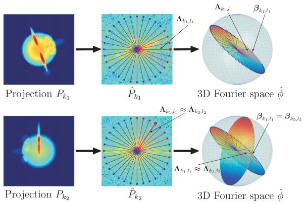
One of the cornerstones of tomography is the Fourier projection-slice theorem, which states that the two-dimensional Fourier transform of a projection image is a planar slice (perpendicular to the beaming direction) of the three-dimensional Fourier transform of the molecule (see, e.g., [Natterer, 2001, p. 11]). The geometry induced by the Fourier projection-slice theorem is illustrated in Figure 1. Any two slices share a common line, i.e., the intersection line of the two planes. Every radial line in the two-dimensional Fourier transform of a projection image is also a radial line in the three-dimensional Fourier transform of the molecule (see for example Λ_k1,l1 in Figure 1). Moreover, there is a 1-to-1 correspondence between each radial line in the three-dimensional Fourier space and its direction vector in ℝ³ (see for example Λ_k1,l1 and β_k1,l1 in Figure 1). The set of all direction vectors (unit vectors in ℝ³) is known as the unit sphere. The radial lines of a single projection image correspond to a great geodesic circle on the unit sphere. The common line property can now be restated as follows: any two different geodesic circles over the unit sphere intersect at exactly two antipodal points. This is demonstrated at the bottom right part of Figure 1.

Figure 1.

Fourier projection-slice theorem and its induced geometry. The Fourier transform of each projection P̂_k corresponds to a planar slice through the three-dimensional Fourier transform φ̂ of the molecule. The Fourier transforms of any two projections P̂_k1 and P̂_k2 share a common line (Λ_k1,l1 and Λ_k2,l2), which is also a ray of the three-dimensional Fourier transform φ̂. Each Fourier ray Λ_k1,l1 can be mapped to its direction vector β_k1,l1. The direction vectors of the Fourier rays Λ_k1,l1 and Λ_k2,l2 that correspond to the common line between P_k1 and P_k2 must coincide, that is, β_k1,l1 = β_k2l2.

Common lines between pairs of projections are usually found using normalized cross correlation [van Heel, 1987]. Given a data set of N projection images P₁(x, y), …, P_N(x, y), one first computes the polar Fourier transform of the images

$${\widehat{P}}_k(\rho ,\alpha )=\frac{1}{{(2\pi )}^2}\int \int P_k(x,y)e^{-i(x\rho cos\alpha +y\rho sin\alpha )}\mathit{dxdy},k=1,\dots ,N,$$ (1)

where 0 ≤ ρ < ∞ and 0 ≤ α < 2π. In practice, this is done by fixing an angular resolution L, and sampling the Fourier transform (1) along L radial lines, at n equispaced points along each radial line. This results in L vectors Λ_k,0, …, Λ_k,L−1 ∈ ℂⁿ, given by

$${\mathbf{\Lambda }}_{k,l}=\left({\widehat{P}}_k\left(\frac{B}{n},\frac{2\pi l}{L}\right),{\widehat{P}}_k\left(\frac{2B}{n},\frac{2\pi l}{L}\right),\dots ,{\widehat{P}}_k\left(B,\frac{2\pi l}{L}\right)\right),$$ (2)

where 1 ≤ k ≤ N, 0 ≤ l ≤ L − 1 and B is the band limit. The DC term (ρ = 0) does not distinguish between lines, because it is shared by all lines independently of the image, and is therefore excluded. To determine the common line between two images P_i and P_j, normalized cross correlations between all L radial lines Λ_i,l1 from the first image with all L radial lines Λ_j,l2 from the second image are computed (overall L² comparisons). However, as the correlation between Λ_i,l1 and Λ_j,l2 has the same value as the correlation between their antipodal lines Λ_i,l1+L/2 and Λ_j,l2+L/2 (where addition of indices is taken modulo L), it follows that the number of distinct correlation values that need to be computed is L²/2, obtained by restricting the index l₁ to take values between 0 and L/2 and letting l₂ take any of the L possibilities (see also [van Heel, 1987] and [Penczek et al., 1994, p. 255]). Equivalently, it is possible to compare real valued 1D line projections of the 2D projection images, instead of comparing radial Fourier lines which are complex valued; these 1D projection lines can be displayed as a 2D image known as a “sinogram” (see [van Heel, 1987; Serysheva et al., 1995]).

The pair of radial lines (or sinogram lines) that has the maximum normalized cross correlation is declared as the common line. In practice, a weighted correlation, which is equivalent to applying a combination of high-pass and low-pass filters is used to determine proximity. As noted in [van Heel, 1987], the normalization is performed so that the correlation coefficient becomes a more reliable measure of similarity between radial lines. The “common lines matrix” C is an N-by-N array whose (i, j) and (j, i) entries store the indices l₁ and l₂, respectively, for which the maximum normalized cross correlation is attained

$$(C(i,j),C(j,i))=\underset{0\le l_1<L/2,0\le l_2<L}{\text{argmax}}\frac{\langle {\mathbf{\Lambda }}_{i,l_1},{\mathbf{\Lambda }}_{j,l_2}\rangle }{\left|\right|{\mathbf{\Lambda }}_{i,l_1}\left|\right|\left|\right|{\mathbf{\Lambda }}_{j,l_2}\left|\right|},\text{for}\text{all}i\ne j.$$ (3)

In other words, C(i, j) is a discrete estimate for where the j’th image intersects with the i’th image. Even with clean images, this estimate will have a small deviation from its ground truth (unknown) value due to discretization errors. With noisy images, large deviations of the estimates from their true values (say, errors of more than 10°) are frequent, and their frequency increases with the level of noise. We refer to common lines that their C(i, j) and C(j, i) values were estimated accurately (up to a given discretization error tolerance) as “correctly detected” common lines, and to the remaining common lines as “falsely detected”. Obviously, we do not know a priori which common lines were correctly detected and which were falsely detected. In the following section we describe a particular voting procedure that attempts to discover the correct common lines.

3. Voting procedure

Suppose that the probability of detecting the correct common line between a pair of images is p. We assume that detection of common lines is very difficult, but not impossible. In other words, p ≪ 1, but at the same time p ≫ 2/L² (2/L² can be achieved by choosing the common lines at random). For example, for p = 1/5 only 20% of the entries in the common lines matrix C in (3) are correct, while the overwhelming majority of 80% of the entries are false. We now describe a simple voting procedure that discovers the correct common lines.

Consider a pair of projection images P_i and P_j. The common line between projections i and j is insufficient to determine the angle α_ij (Figure 2) between their corresponding three-dimensional planes. However, the common lines between three projections i, j and k uniquely determines the relative orientation of the three projections up to handedness (chirality). This is the basis of the angular reconstitution method [van Heel, 1987].

Figure 2.

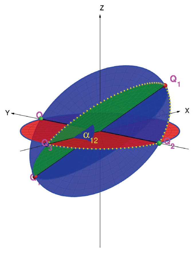
Angular Reconstitution: the common lines between P₁, P₂, P₃ uniquely determine the angle α₁₂ between P₁ and P₂ as well as the three intersection points Q₁₂, Q₁₃ and Q₂₃ (“triangle”) of their corresponding great circles on the unit sphere (up to some three-dimensional rotation and possibly a reflection).

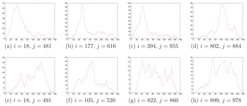
First, let us consider the case where the common line between projections i and j was correctly identified. Given the pair (i, j), we consider all N − 2 different triplets of the form (i, j, k) (k = 1, 2, …, N, k ≠ i, j). Each projection k can vote only once and all votes have equal weight. By the angular reconstitution method, the triplet (i, j, k) determines the angle α_ij between projections i and j. With probability p² the common lines between projections i and k and between projections j and k are correct. For all such “good” k’s, the resulting angle α_ij is the same. With probability 1 − p² one of the common lines (either (i, k) or (j, k)) is wrong and the resulting angle α_ij is random or non-physical (non-physical common lines are explained in Section 4). There are p²(N − 2) “good” third projections on average that all give the same angle. The resulting histogram of the angle α_ij is therefore a mixture of a flat distribution (random angles) and a delta-spike at the correct angle. This is demonstrated using simulated data in Section 5, and is illustrated in Figure 5. On the other hand, if the common line between i and j is incorrect, then triplets of the form (i, j, k) give rise to random (or non-physical) angles α_ij. The histogram of the angle in this case is flat without spikes.

Figure 5.

Smoothed histograms of the angle (in degrees) between pairs of projections. The plots were generated using N = 1000 projections with SNR=1/16. Top row corresponds to pairs of projections whose common lines were correctly identified. Bottom row corresponds to pairs of projections whose common lines were misidentified. Note the different scale of the y-axis in the two cases, indicating much higher peaks for correctly identified common-lines.

We can distinguish between the two typical histograms (completely random versus random + spike) if the spike is significantly high. In other words, we are able to tell that a common line was correctly identified whenever enough projections voted in the same way. That is, to be able to tell the “good” from the “bad”, the spike must consist of enough votes, which happens if the condition

$$p^2(N-2)\gg 1$$ (4)

is satisfied. This shows that even at low detection rates, the larger the data set the better. For example, when p = 1/5 and N = 10000 we expect a spike of size ≈ 400.

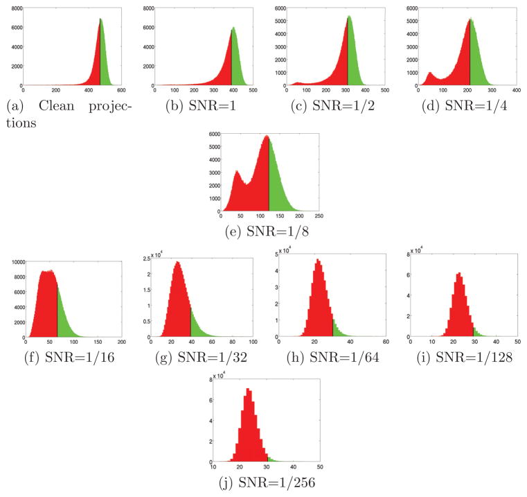
In practice, we have no estimate for the value of p. Instead, we plot for each pair of projections its angle histogram, and record the height of its peak. Following the discussion above, even though we do not know p, the angle histogram for pairs for which the common line was correctly identified will exhibit a higher peak than for pairs for which the common line was misidentified. This is true as long as p is not too small. Thus, once we compute the peak of the angle histogram for each pair of projections, we plot the histogram of the peaks. Pairs of projections that correspond to the right-hand-side of the peaks histogram are those for which the peak of their angle histogram was highest. It is thus more likely that the common line between those projections was correctly identified. We demonstrate this in Section 5. For explanatory purposes, we assume in the simulations in Section 5 that p is known, to demonstrate quantitatively the performance of the algorithm. This assumption is not required when processing experimental data. In the experimental setup we first plot the histogram of the modes as shown in Figures 8 and 9. The choice of the threshold is straightforward if this histogram exhibits two distinguished modes (clearly visible in Figures 8d and 8e), with the left mode (smaller values) corresponding to falsely identified common lines and the right mode (larger values) corresponding to the correctly identified common lines (see further discussion in Section 5.1).

Figure 8.

Histogram of peaks for N = 1000 and various levels of noise. The top p/2 percentile of each histogram is marked in Green, the bottom 1 − p/2 percentile is marked in Red, and the boundary between the regions is marked as a black vertical line. The location of the boundary is the minimal peak height to be considered by the algorithm as a correctly identified common line. Note how this threshold value decreases as the SNR decreases. The algorithm assumes that the correct common lines are concentrated in the Green area and that the wrong common lines are concentrated in the Red area.

Figure 9.

Histogram of peaks for SNR = 1/16 for N = 100, 500, 1000, 5000.

If two modes are not clearly visible in the histogram of the modes, then we try a few different threshold values using the following consideration. Equation (4) gives a necessary condition for the voting procedure to succeed, from which it follows that if (the unknown) p is below $1/\sqrt{N}$ then the method has no chance to succeed. The threshold value should therefore be one of the top $100\%/\sqrt{N}$ highest histogram modes. As there are N(N − 1)/2 possible threshold values, the threshold must be one of the O(N^3/2) highest modes. We therefore try a few different threshold values corresponding to thresholding at the top $\gamma \frac{100\%}{\sqrt{N}}$ percentile, with γ = 2, 4, 8, 16. For example, for N = 3000 the threshold is varied from as high as the top 3.6% percentile to as low as the top 29.2% percentile.

4. Disqualified votes and angular assignment

Not all triplets of common lines can be realized as planes whose common lines are the given triplet. Such inconsistent triplets lead to non-physical angles, as we now explain. As illustrated in Figure 2, the three great circles corresponding to projections 1, 2 and 3 intersect on the unit sphere at Q₁₂, Q₁₃ and Q₂₃ (Q_ij is the intersection of the two circles corresponding to projections i and j; there are also three antipodal intersection points). The three common lines determine the distances between the three intersection points. Those distances are always between 0 and 2 (the largest distance between points on the unit sphere).

Clearly, three points Q₁₂, Q₁₃, Q₂₃ in the unit sphere that are not collinear will always form a unique triangle. In practice, however, we have no access to the coordinates of Q₁₂, Q₁₃, Q₂₃. Instead, the common lines data translate (as we explain below) to distances between the three points. These observed distances are noisy realizations of the true distances, as is the case when the estimation of the common lines is incorrect. With noisy distances it is not always the case that three distances define a triangle on the unit sphere. We proceed to verify the exact condition that guarantees for three input distances between 0 to 2 to form a triangle that can be lay in the unit sphere.

For three distances to form a triangle, they must satisfy the triangle inequality. It turns out that the triangle inequality is not sufficient to determine the triangle, because the three points must lie on the unit sphere as well. For example, the distances 2, 2, 2 satisfy the triangle inequality, but the corresponding triangle is too big to be placed on the unit sphere. The exact condition that guarantees a successful triangulation is obtained by using either linear algebra or geometry. We first give the linear algebra derivation.

The three dot products between the three points Q_ij, Q_ik, and Q_jk are obtained from the common lines between projections i, j, and k by

$$\langle Q_{ij},Q_{ik}\rangle =cos(2\pi (C(i,j)-C(i,k))/L),$$ (5)

where C(i, j) is the index of the common line between projections i and j at the plane of projection i. Since the points are on the unit sphere, we have 〈Q_ij, Q_ij〉 = 1. The Gram matrix of Q₁₂, Q₁₃, Q₂₃ is the 3-by-3 matrix of their dot products given by

$$\left(\begin{array}{ccc}1& \langle Q_{23},Q_{13}\rangle & \langle Q_{23},Q_{12}\rangle \\ \langle Q_{13},Q_{23}\rangle & 1& \langle Q_{13},Q_{12}\rangle \\ \langle Q_{12},Q_{23}\rangle & \langle Q_{12},Q_{13}\rangle & 1\end{array}\right)=\left(\begin{array}{ccc}1& a& b\\ a& 1& c\\ b& c& 1\end{array}\right),$$ (6)

where

$$\begin{array}{l}a=cos(2\pi (C(3,2)-C(3,1))/L),\\ b=cos(2\pi (C(2,3)-C(2,1))/L),\\ c=cos(2\pi (C(1,3)-C(1,2))/L).\end{array}$$ (7)

We define

$$G=\left(\begin{array}{ccc}1& a& b\\ a& 1& c\\ b& c& 1\end{array}\right).$$ (8)

Note that the matrix G in (8) can always be formed by combining the common lines information with (7). We want to find a condition under which there exist coordinates Q₁₂, Q₁₃, Q₂₃ such that (6) holds. A necessary and sufficient condition in that the matrix (8) is positive definite. To see this, suppose that we can write G in (8) as a matrix of dot products as in (6). Then, G = Q^T Q where Q = (Q₂₃, Q₁₃, Q₁₂) is the matrix having the coordinates of Q₂₃, Q₁₃, and Q₁₂ as its columns, which immediately shows that G is positive definite. Conversely, if G is positive definite, then the Cholesky decomposition [Golub and Van Loan, 1984] of G is in the form of G = Q^T Q and so (6) holds. We proceed to derive the condition for G to be positive definite.

We begin with examining the trace of G

$$\text{Tr}(G)=3={\lambda }_1+{\lambda }_2+{\lambda }_3,$$ (9)

where λ₁ ≥ λ₂ ≥ λ₃ are the sorted eigenvalues of G, which immediately implies λ₁ > 0. Since |a|, |b|, |c| ≤ 1 it follows that the sums of the absolute values of the rows of G are bounded by 3: 1 + |a|+ |b| ≤ 3, 1 + |a|+ |c| ≤ 3 and 1 + |b|+ |c| ≤ 3. By the Gershgorin circle theorem [Golub and Van Loan, 1984] it follows that λ₁ ≤ 3. Combining this with (9) we obtain that λ₂ + λ₃ ≥ 0. Therefore, λ₂ ≥ 0 (because 2λ₂ ≥ λ₂ + λ₃ ≥ 0). A necessary and sufficient condition for positive definiteness is that all eigenvalues are positive. Since we have already established that λ₁ ≥ λ₂ ≥ 0, it remains to require that the smallest eigenvalue is positive, that is, to require that λ₃ > 0. To that end, we use the determinant of G which equals the product of the eigenvalues: det(G) = λ₁λ₂λ₃. In our case, the determinant is given by

$$det(G)=1-(a^2+b^2+c^2)+2\mathit{abc}.$$ (10)

We conclude that the condition for positive definiteness is

$$1+2\mathit{abc}>a^2+b^2+c^2.$$ (11)

The condition (11) explains for example why the distances 2, 2, 2 corresponding to a = b = c = −1 are not realizable on the sphere. Only triplets (i, j, k) that satisfy the condition (11) are physical and eligible to vote. All other votes are disqualified. Though it may be tempting to think that condition (11) is violated only when projections are nearby and their common lines lie very close to each other and therefore are not informative anyway, even moderate angles, such as a = b = c = −1/2 lead to violations.

An alternative approach for deriving condition (11) uses the geometry of the sphere. We may assume that the circle corresponding to projection 1 lies in the xy-plane, so it has the parametrization (cos θ₁, sin θ₁, 0) (0 ≤ θ₁ < 2π). By an arbitrary choice of the coordinate system, the intersection point of projections 1 and 2 is

$$Q_{12}=(1,0,0),$$

and the intersection point of projections 1 and 3 is

$$Q_{13}=(c,\sqrt{1-c^2},0).$$

Since the great circle that corresponds to projection 2 goes through Q₁₂ = (1, 0, 0), it follows that its parametrization is given by (cos θ₂, cos α₁₂ sin θ₂, sin α₁₂ sin θ₂) (0 ≤ θ₂ < 2π), where α₁₂ is the angle between projections 1 and 2 (see Figure 2). In particular, from 〈Q₁₂, Q₂₃〉 = b, we get

$$Q_{23}=(b,\sqrt{1-b^2}cos{\alpha }_{12},\sqrt{1-b^2}sin{\alpha }_{12}).$$

Taking the dot product between Q₁₃ and Q₂₃ we obtain

$$\begin{array}{l}a=\langle Q_{13},Q_{23}\rangle =(c,\sqrt{1-c^2},0)·(b,\sqrt{1-b^2}cos{\alpha }_{12},\sqrt{1-b^2}sin{\alpha }_{12})\\ =bc+\sqrt{1-b^2}\sqrt{1-c^2}cos{\alpha }_{12},\end{array}$$

from which cos α₁₂ is extracted

$$cos{\alpha }_{12}=\frac{a-bc}{\sqrt{1-b^2}\sqrt{1-c^2}}.$$ (12)

The condition cos² α₁₂ ≤ 1 is equivalent to (11). The voting algorithm is outlined in Algorithm 1.

Algorithm 1.

Voting algorithm

Input: N × N common lines matrix C defined in (3).
1:	Define T equally spaced angles between 0° and 180°: αt = 180t/T, t = 0, …, T − 1.
2:	for k1 = 1 to N do
3:	for k2 = k1 + 1 to N do
4:	Initialize the histogram vector h of length T to zero.
5:	for k3 = 1 to N do
6:	Compute a, b, and c using (7) and the values C(k1, k2), C (k2, k1), C (k1, k3), C(k3, k1), C (k2, k3), C (k3, k2).
7:	if condition (11) is satisfied then
8:	Compute α12 using (12).
9:	Update the histogram h using Gaussian smoothing
	$h(t)=h(t)+\frac{1}{\sqrt{2\pi {\sigma }^2}}{e}^{-{({\alpha }_t-{\alpha }_{12})}^2/(2{\sigma }^2)}$, t = 0, …, T − 1, σ = 180/T.
10:	end if
11:	end for
12:	Find and store the mode of the histogram: P (k1, k2) = maxt h(t)
13:	end for
14:	end for
15:	Declare pairs (k1, k2) with large values of P(k1, k2) as good common lines.

As stated, Algorithm 1 returns pairs of projection images (k₁, k₂) for which the common lines between them are suspected to be identified correctly, but the algorithm does not assign Euler angles to the projections. The latter has to be done separately, after termination of the voting algorithm. The main issue here is that although the voting procedure finds the correct common lines, it may happen that it wrongly detects false common lines as being correct. Such outliers may be post-identified using the energy minimization procedure of [Penczek et al., 1996]. Another possibility is to squeeze out more information out of the voting algorithm, by noting that for good common lines, the location of the mode of the histogram gives the angle between the planes and this information can be incorporated into the energy minimization framework. A different method that we use in this paper to solve the angular assignment problem is described in the technical report [Coifman et al., 2007]. Briefly speaking, this method uses the good common lines reported by the voting algorithm to construct an N × N sparse matrix whose top three eigenvectors provide an estimate for the Euler angles. We are currently developing an alternative spectral and semidefinite programming relaxation methods that show potential of handling a larger percentage of outliers. These relaxation techniques will be reported in a separate publication [Singer and Shkolnisky, 2009].

The voting algorithm may also be useful in detecting non-particle images, which is a problem often encountered in practice, as automatic particle picking is known to pick a large number (up to 20–25%) of non-particles. All these images will smear the average classes or will cluster into some non-particle classes which will be compared to the rest of good-particle classes during the voting procedure. The voting algorithm is expected to find that such bad non-particle classes have a relatively small number of good common lines with the remaining particle classes. This provides a way to identify non-particle classes, and later reconstruction procedures should only use classes whose number of good common lines exceeds a certain threshold.

5. Results

We conducted several numerical experiments to test the performance of the voting procedure. In Section 5.1 we apply the algorithm on simulated electron-microscope projections. This allows us to demonstrate quantitatively the performance of the algorithm. Then, in Section 5.2, we apply the algorithm on a real electron microscope data set, obtaining three-dimensional models directly from a large number of class averages.

5.1. Simulations

We applied the voting algorithm on sets of simulated projections of a ribosomal subunit, containing N = 100, 500, 1000, and 5000 projections. For each N, we generated N noise-free centered projections of the particle at uniformly distributed random orientations. Specifically, the projection orientations were obtained by sampling the set of all three-dimensional rotations, known as the rotation group SO(3), uniformly at random. Each projection was of size 129 × 129 pixels. Next, we fixed a signal-to-noise ratio (SNR), and added to each clean projection additive Gaussian white noise of the prescribed SNR. The SNR in all our experiments is defined by

$$\text{SNR}=\frac{\text{Var}(\mathit{Signal})}{\text{Var}(\mathit{Noise})},$$ (13)

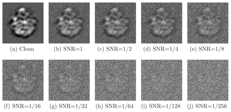
where Var is the variance (energy), Signal is the clean projection image and Noise is the noise realization of that image. Figure 3 shows one of the projections at different SNR levels. The SNR values used throughout this experiment were 2^−k with k = 0, …, 9. Clean projections were generated by setting SNR = 2²⁰.

Figure 3.

Simulated projection with various levels of additive Gaussian white noise.

The first step of the experiment was to determine the values of the angular resolution L and the radial discretization n of the radial Fourier lines. Computing the normalized correlation between a single pair of radial lines takes the order of n operations. As mentioned earlier, the number of correlations that need to be computed in order to detect the common line between two images is L²/2. It follows that the complexity of finding a single common line is of the order of nL², and clearly the algorithm is faster with smaller values of L and n. On the other hand, choosing L and n to be too small will prevent common line routines from detecting a good approximation of the true common line due to poor resolution in either the angular or radial directions. In all subsequent experiments we use L = 72 and n = 100, which corresponds to an angular resolution of 5°.

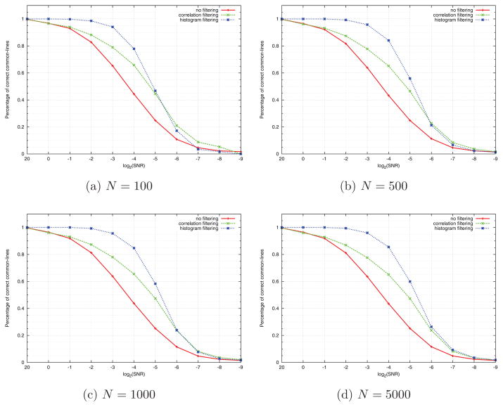
Once L and n have been fixed, we took sets of noisy projections with a given SNR, and constructed for each set its corresponding common lines matrix. The percentage of correctly identified common lines in each matrix is plotted against the SNR for various values of N in Figures 4a–4d, using the curve designated by “no filtering”. Each such curve gives the probability p of detecting common lines between projections as a function of the SNR. In all experiments we consider the common lines between two projections as correctly identified, if the estimated common lines deviate from the true ones by up to 10°.

Figure 4.

Comparing correlation filtering and histogram filtering for (a) N = 100, (b) N = 500, (c) N = 1000, (d) N = 5000.

We then applied “correlation filtering” to the common lines matrices, that is, we retained only common lines whose correlations are among the highest p/2 percentile of correlations. Specifically, we retained a common line (Λ_i,l1, Λ_j,l2) only if the normalized correlation between rays Λ_i,l1 and Λ_j,l2 is one of the top p/2 × N (N − 1)/2 correlation values. We then plotted the percentage of correct common lines among the retained common lines. This is shown in Figures 4a–4d using the curve designated by “correlation filtering”. Obviously, this filtering improves the detection rate of common lines. Note that since there are only pN(N − 1)/2 correct common lines, there is no point in retaining more than that, as any larger number would necessarily increase the number of errors. We used as a threshold half this number.

Finally, we filtered the original common lines matrices using the voting procedure, which we also refer to as “histogram filtering”. The histogram filtering consists of several steps. The first step is to compute for each pair of projections (P_i, P_j) the angle induced between them by all third projections. This gives a series of N − 2 estimates for the angle α_ij between P_i and P_j. If the common line between projections P_i and P_j was correctly identified, we expect these estimates to be centered around the true angle between P_i and P_j. That is, we expect the histogram of the estimates to exhibit a peak at the correct angle.

To find this peak, we use a Gaussian kernel to obtain a smooth density estimation for the angle between P_i and P_j, followed by mode seeking over a discrete set of T = 60 equally spaced angles between 0° to 180°. We choose the width of the Gaussian kernel as σ = 3° (see also steps 1 and 9 in Algorithm 1). The Gaussian smoothing serves as a simple way for binning the histogram such that close-by angle estimates are combined into a single peak. In Figure 5 we show several examples for the smoothed histogram of the angle between pairs of projections. These histograms were obtained from the experiment that corresponds to N = 1000 and SNR = 1/16. Figures 5a–5d show smoothed histograms for pairs of projections where the common lines were correctly identified. Figures 5e–5h correspond to pairs of projections for which the common lines were misidentified. Note the different scaling of the y-axis between the cases of correct and incorrect identification of common lines.

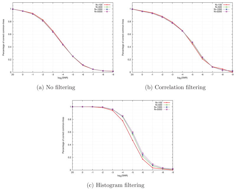
As explained at the end of Section 3, we record for each angle histogram the height of its peak (step 12 in Algorithm 1), and compute the histogram of the peaks. We then retain only common lines whose peaks are among the p/2 percentile of highest peaks (p is the probability of detecting a correct common line, obtained from the curve designated by “no filtering” in Figures 4a–4d). The resulting percentage of correct common lines is shown in Figures 4a–4d using the curve designated by “histogram filtering”. As evident from Figures 6a–6c, increasing N improves the performance the histogram filtering, but not of the correlation filtering. However, as Figures 4a–4d show, histogram filtering is consistently superior to correlation filtering.

Figure 6.

Common lines detection rate as a function of the SNR, for various values of N, when using (a) no filtering, (b) correlation filtering, (c) histogram filtering.

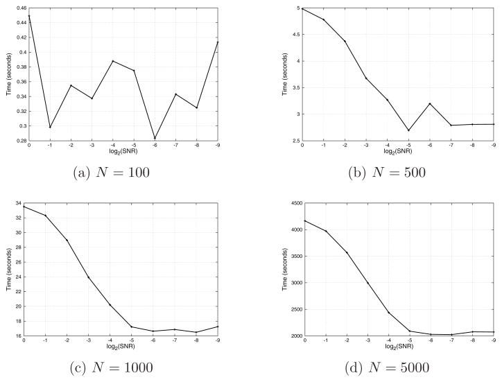
All experiments in this subsection were executed on a Linux machine with 16 Xeon 2.93GHz cores and 48GB of RAM. The algorithm for detecting common lines between projections was implemented in MATLAB, thus taking partial advantage of multiprocessing in computations that use the Basic Linear Algebra Subroutines (BLAS) library. This gives some degree of parallelization in computing cross-correlations, but our experience shows that the current implementation never exceeds 200% utilization (that is, cannot use more than 2 cores at any given time). The running times for computing the common lines matrices were 12.12 seconds for N = 100, 169.34 seconds for N = 500, 658.38 seconds for N = 1000, and 15907.43 seconds for N = 5000. The voting procedure was parallelized in C to take advantage of all computing cores, and its speed scales linearly with the number of CPUs. Though it is an O(N³) procedure, the constant associated with it is very small, and thus the algorithm is practical for rather large N (like N = 5000). The reason for the small constant is that given a pair of projections, the first step of the voting checks all third projections and disqualifies non-physical angles. This test requires computing a simple formula for checking condition (11) and is very fast. In the noise levels typically present in class averages of real microscope images, only a few projections pass that test. Thus, updating the histogram never involves O(N) angles but rather much less. Figure 7 shows the running times required for histogram filtering as a function of the SNR. It is clear that histogram filtering gets faster as the SNR decreases, since more triplets are being disqualified, as explained in Section 4.

Figure 7.

Running time (in seconds) of histogram filtering as a function of the SNR.

Figures 8a–8j show the histograms of peaks for N = 1000 projections and various levels of SNR. As can be seen from the figures, for lower noise levels (see for example Figures 8d and 8e), the histograms consist of two well-separated distributions (bumps) – the right peak corresponds to the average peak height of histograms of correctly identified common lines; the left peak corresponds to the average peak height of histograms of misidentified common lines. As the noise level increases, the two distributions start to overlap. Figures 9a–9d show the histogram of peaks for a fixed SNR = 1/16 and various values of N. As N increases, it becomes possible to resolve the peak that corresponds to misidentified common lines from the peak that corresponds to correctly identified common lines.

5.2. Reconstruction from ribosome images

A set of micrographs of E. coli 50S ribosomal subunits was provided by M. van Heel. These images were acquired with a Philips CM20 at defocus values between 1.37 and 2.06 μm; they were scanned at 3.36 Å/pixel, and particles were picked using the automated particle picking algorithm in EMAN Boxer. All subsequent image processing was performed with the IMAGIC software package [Stark, H. et al., 2002; van Heel, M. et al., 1996]. The particle images were phase-flipped to remove the phase-reversals in the CTF and bandpass filtered at 1/150 Å and 1/8.4 Å. The variance-normalized images were translationally aligned with the rotationally-averaged total sum.

Without rotational alignment, the 27,121 particle images were classified using the MSA function into sets of 750, 1500 and 3000 classes, and the class means were used for the voting algorithm. In parallel, the IMAGIC routines were used to perform multiple cycles of multireference alignment and classification, reconstruction using angular reconstitution, and model refinement.

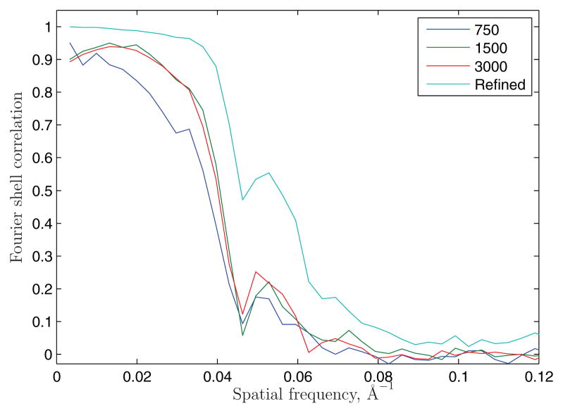
A comparison of the refined model and the three models obtained directly from the sets of 3000, 1500 and 750 class averages is shown in Figure 10. Each class average is formed from ≈ 9, 18 or 36 particle images, respectively. The set of 750 class averages yielded the lowest-quality reconstruction; this is to be expected because the number of classes does not sufficiently sample the three Euler angles of orientation. Nevertheless this and the other two models computed directly from the common-lines assignments represent excellent ab initio models. Figure 11 evaluates the model agreement by Fourier shell correlations (FSCs). The FSC of the refined model, obtained from reconstructions of two halves of the data set, shows a nominal resolution of about 15Å at the 0.5 threshold criterion and 11.7Å using the 3σ criterion. FSCs were also computed between the refined model and the models obtained directly from the voting algorithm. The ab initio models agree with the refined model up to 25Å, with the 1500 and 3000-class reconstructions being slightly better than the 750-class reconstruction. Reconstructions failed when using 500 class averages due to excessive averaging, and for sets of 5000 and 7000 class averages due to the low detection rate of common lines.

Figure 10.

Comparison of a refined model of the 50S ribosomal subunit with direct reconstructions from N = 750, 1500 and 3000 class averages. The refined model is from an Imagic reference-based alignment of the 27,121 particle data set used in this study and refined to 11.7Å resolution (3σ criterion). The remaining structures were generated directly from the voting-derived common line assignments following classification into the given numbers of input classes. The voting-based structures, for the sake of comparison, were soft masked and filtered to 15Å resolution. The structures were also flipped about the z-axis such that their handedness is consistent with the X-ray structure [Ban N. et al., 2000] and shown as the Imagic-generated 3D volumes.

Figure 11.

Fourier shell correlations of the various reconstructions.

6. Computational complexity

As stated, Algorithm 1 has a computational complexity of O(N³), which may be computationally prohibitive with datasets as large as N = 10⁵. In fact, already the computation of the N × N common lines matrix is quadratic in N and may be too time consuming for large N, as it requires the computation of O(L²) normalized correlations for each pair of images, and the computation of each normalized correlation is O(n), where N is the number of discretization points of the radial Fourier lines, so the overall complexity of computing the common lines matrix is O(N²L²n). There are at least three possible ways in which the voting algorithm may be accelerated.

First, since the number of good common lines needed for assigning the Euler angles of N projections is O(N), it follows that if p is the detection rate, then the expected number of projection pairs (k₁, k₂) that need to be examined until O(N) good common lines are collected is O(N/p) (here, the enumeration over the pairs (k₁, k₂) should not progress sequentially like (1, 2), (1, 3), (1, 4), …, as currently done in Algorithm 1, but rather in a random fashion). Since p is at least as large as $1/\sqrt{N}$, for otherwise condition (4) is violated, it follows that N/p is bounded by N^1.5. Thus, the number of pairs (k₁, k₂) for which we need to make a histogram is only O(N^1.5), and since histogram preparation takes O(N), it follows that the overall complexity of a careful implementation of the voting procedure would be O(N^2.5), saving a factor of $\sqrt{N}$ on the naïve implementation.

Second, the histogram updating can be stopped once enough votes had been cast. Put in another way, from equation (4) it follows that the number of votes needed, denoted K, should satisfy K = O(1/p²). The overall complexity would be the number of pairs (k₁, k₂) times K, or the number of pairs times 1/p². Since the number of pairs needed is O(N/p), the overall complexity of the algorithm is O(N/p³). The maximum complexity is obtained when $p=1/\sqrt{N}$ and then N/p³ = N^2.5, but at the other extreme (p = 1) we get a linear algorithm (which is not that surprising, as in this case one can simply use a sequential implementation of van Heel’s angular reconstitution method to assign all angles). In practice, however, we do not know the value of p, so the very careful implementation would also need to estimate p “on the fly”, for example, by noting after how many pairs (k₁, k₂) a first spiky histogram was obtained.

Third, in order to obtain an ab initio coarse structure, it is usually not necessary to find the angular assignment of all N projections. A coarse structure can be obtained from a fewer number N′ of projections (N′ < N) and can be later refined using the entire image collection. While the number of votes for each histogram can still be as large as N, the number of pairs (k₁, k₂) can be limited to N′ (N′ − 1)/2 instead of N(N − 1)/2. For example, if the number of projections is N = 10⁵, and we choose N′ = 10², we get a computational savings factor of 10⁶.

At the moment, our implementation follows the description of Algorithm 1 without the computational savings discussed above.

7. Summary and discussion

We presented a simple and efficient voting procedure that makes use of the geometry rendered by the Fourier projection-slice theorem to identify the correct common lines even in the presence of many other falsely detected common lines. The quality of a common line is determined by all other images. Our method succeeds even at a low detection rate of common lines and would therefore allow common lines-based methods to succeed in lower SNR. It would allow, for example, to use noisier class averages, where each class consists of fewer projections.

The voting procedure can be easily adjusted to handle cases in which there are several common line candidates: for each candidate we produce a histogram and choose the one (if any) that shows an identifiable spike.

We note that the method may also be useful for the heterogeneity problem. In theory, if we pick a pair of projections corresponding to different types, then all triplets containing the pair should be incoherent and produce random angles. In practice, however, the problem of heterogeneity is more difficult. Projections of different types are very similar and can easily fool the common line test. This is especially true when dealing with class averages that may contain projections from different types.

Our experience with simulative data shows that the detection rate of common lines between a fixed pair of images exhibits a phase transition behavior. Once the SNR goes below a certain threshold, the detection rate decays exponentially quickly. This is in agreement with the threshold phenomenon in non-linear estimation theory that was developed originally for radar range estimation [Zakai, M. and Ziv, J., 1969; Ziv, J. and Zakai, M., 1969]. In our case, the threshold is different from one pair of images to the other, and so some common lines may be correctly detected while others are not. In other words, although the detection of common lines between a fixed pair of images exhibits a sharp threshold phenomenon as a function of the SNR, the threshold region is much wider and smoother for the entire data set since we are comparing many different pairs with different thresholds.

Improved filters and correlation tests for common line detection can push the detection threshold lower and therefore significantly improve the performance of any common lines based algorithm like the one presented in this paper. We believe that constructing improved comparison tests, such as developing tests based on some clever feature selection to replace simple correlation, is a research direction that should be strongly pursued.

References

- Ban N, Nissen P, Hansen J, Moore PB, Steitz TA. The complete atomic structure of the large ribosomal subunit at 2.4 å resolution. Science. 2000;289:905–920. doi: 10.1126/science.289.5481.905. [DOI] [PubMed] [Google Scholar]
- Chiu W, Baker LM, Jiang W, Dougherty M, Schmid MF. Electron cryomicroscopy of biological machines at subnanometer resolution. Structure. 2005;13(3):363–372. doi: 10.1016/j.str.2004.12.016. review. [DOI] [PubMed] [Google Scholar]
- Coifman RR, Shkolnisky Y, Sigworth FJ, Singer A. Yale University, Department of Computer Science; 2007. Cryo-em structure determination through eigenvectors of sparse matrices. Technical Report 11, 1–42. URL http://www.cs.yale.edu/publications/techreports/tr1389.pdf. [Google Scholar]
- Farrow M, Ottensmeyer P. A posteriori determination of relative projection directions of arbitrarily oriented macrmolecules. Journal of the Optical Society of America A: Optics, Image Science, and Vision. 1992;9 (10):1749–1760. [Google Scholar]
- Frank J. Three-Dimensional Electron Microscopy of Macromolecular Assemblies: Visualization of Biological Molecules in Their Native State. Oxford: 2006. [Google Scholar]
- Golub GH, Van Loan CF. Johns Hopkins series in the mathematical sciences. The Johns Hopkins University Press; 1984. Matrix Computation. [Google Scholar]
- Goncharov AB. Integral geometry and three-dimensional reconstruction of randomly oriented identical particles from their electron microphotos. Acta Applicandae Mathematicae. 1988;11:199–211. [Google Scholar]
- Henderson R. Realizing the potential of electron cryo-microscopy. Q Rev Biophys. 2004;37(1):3–13. doi: 10.1017/s0033583504003920. review. [DOI] [PubMed] [Google Scholar]
- Ludtke SJ, Baker ML, Chen DH, Song JL, Chuang DT, Chiu W. De novo backbone trace of GroEL from single particle electron cryomicroscopy. Structure. 2008;16 (3):441–448. doi: 10.1016/j.str.2008.02.007. [DOI] [PubMed] [Google Scholar]
- Mallick SP, Agarwal S, Kriegman DJ, Belongie SJ, Carragher B, Potter CS. Structure and view estimation for tomographic reconstruction: A Bayesian approach. Computer Vision and Pattern Recongnition (CVPR) II. 2006:2253–2260. [Google Scholar]
- Natterer F. Classics in Applied Mathematics. SIAM: Society for Industrial and Applied Mathematics; 2001. The Mathematics of Computerized Tomography. [Google Scholar]
- Penczek PA, Grassucci RA, Frank J. The ribosome at improved resolution: new techniques for merging and orientation refinement in 3d cryo-electron microscopy of biological particles. Ultramicroscopy. 1994;53:251–270. doi: 10.1016/0304-3991(94)90038-8. [DOI] [PubMed] [Google Scholar]
- Penczek PA, Zhu J, Frank J. A common-lines based method for determining orientations for N > 3 particle projections simultaneously. Ultramicroscopy. 1996;63:205–218. doi: 10.1016/0304-3991(96)00037-x. [DOI] [PubMed] [Google Scholar]
- Salzman DB. A method of general moments for orienting 2d projections of unknown 3d objects. Computer vision, graphics, and image processing. 1990;50:129–156. [Google Scholar]
- Serysheva II, Orlova EV, Chiu W, Sherman MB, Hamilton SL, van Heel M. Electron cryomicroscopy and angular reconstitution used to visualize the skeletal muscle calcium release channel. Nature Structural Biology. 1995;2:18–24. doi: 10.1038/nsb0195-18. [DOI] [PubMed] [Google Scholar]
- Singer A, Shkolnisky Y. Three-dimensional structure determination from common lines in cryo-em by eigenvectors and semidefinite programming. 2009 doi: 10.1137/090767777. submitted. [DOI] [PMC free article] [PubMed] [Google Scholar]
- Stark H, Rodnina MV, Wieden HJ, Zemlin F, Wintermeyer W, van Heel M. Ribosome interactions of aminoacyl-tRNA and elongation factor Tu in the codon-recognition complex. Nature Structural Biology. 2002;9:849–854. doi: 10.1038/nsb859. [DOI] [PubMed] [Google Scholar]
- Vainshtein B, Goncharov A. Determination of the spatial orientation of arbitrarily arranged identical particles of an unknown structure from their projections. Proc. llth Intern. Congr. on Elec. Mirco; 1986. pp. 459–460. [Google Scholar]
- van Heel M. Angular reconstitution: a posteriori assignment of projection directions for 3D reconstruction. Ultramicroscopy. 1987;21(2):111–123. doi: 10.1016/0304-3991(87)90078-7. [DOI] [PubMed] [Google Scholar]
- Van Heel M, Orlova EV, Harauz G, Stark H, Dube P, Zemlin FMS. Angular reconstitution in three-dimensional electron microscopy: historical and theoretical aspects. Scanning Microscopy. 1997;11:195–210. [Google Scholar]
- van Heel M, Harauz G, Orlova EV, Schmidt R, Schatz M. A new generation of the IMAGIC image processing system. Journal of Structural Biology. 1996;116 (1):17–24. doi: 10.1006/jsbi.1996.0004. [DOI] [PubMed] [Google Scholar]
- Wang L, Sigworth FJ. Cryo-em and single particles. Physiology (Bethesda) 2006;21:13–18. doi: 10.1152/physiol.00045.2005. review. [DOI] [PubMed] [Google Scholar]
- Zakai M, Ziv J. On the threshold effect in radar range estimation. IEEE Transactions on Information Theory. 1969;15 (1):167–170. [Google Scholar]
- Zhang X, Settembre E, Xu C, Dormitzer PR, Bellamy R, Harrison SC, Grigorieff N. Near-atomic resolution using electron cryomicroscopy and single-particle reconstruction. Proceedings of the National Academy of Sciences. 2008;105 (6):1867–1872. doi: 10.1073/pnas.0711623105. [DOI] [PMC free article] [PubMed] [Google Scholar]
- Ziv J, Zakai M. Some lower bounds on signal parameter estimation. IEEE Transactions on Information Theory. 1969;15 (3):386–391. [Google Scholar]