

Abstract
The basic reproduction number R 0 is one of the most important concepts in modern infectious disease epidemiology. However, for more realistic and more complex models than those assuming homogeneous mixing in the population, other threshold quantities can be defined that are sometimes more useful and easily derived in terms of model parameters. In this paper, we present a model for the spread of a permanently immunizing infection in a population socially structured into households and workplaces/schools, and we propose and discuss a new household-to-household reproduction number R H for it. We show how R H overcomes some of the limitations of a previously proposed threshold parameter, and we highlight its relationship with the effort required to control an epidemic when interventions are targeted at randomly selected households.
Keywords: epidemic models, stochastic models, threshold parameters, households, workplaces and schools, social structure
1. Introduction
Compartmental models of infectious disease spread have had a long and successful history in epidemiology (Kermack & McKendrick 1927; Bailey 1975; Anderson & May 1991; Diekmann & Heesterbeek 2000; Hethcote 2000), thanks to their mathematical tractability and the flexibility they show in allowing the model to be enriched by more realistic features that characterize the population and the infection under investigation (e.g. Anderson & May 1991; Diekmann & Heesterbeek 2000). However, they are usually based on some unrealistic assumptions, the most crucial of which is often the oversimplified description of the interaction between individuals. In fact, it is well known that the social structure of a population influences the dynamics of an epidemic spreading through it (e.g. Becker et al. 1995; Edmunds et al. 1997).
Besides increased realism, more complex models than those assuming homogeneous mixing are also necessary to investigate the effects of targeted control policies, which are usually less expensive and more efficient than control policies applied to the whole population (e.g. Roberts 2004; Aldis 2005; Becker et al. 2005; Ferguson et al. 2005, 2006; Longini et al. 2005; Roberts 2007). For example, vaccination is more likely to be delivered to entire households instead of randomly selected individuals (Becker & Dietz 1995; Becker et al. 1995; Becker & Utev 1998; Wu et al. 2006; Fraser 2007). Furthermore, during an emerging outbreak, control policies such as quarantine and prophylactic treatment are often targeted at households (Wu et al. 2006; Fraser 2007), while social distancing measures can involve, among other actions, school and workplace closure (e.g. Ferguson et al. 2005, 2006; Cauchemez et al. 2008).
Unfortunately, the increased realism gained by adding a more detailed social structure to a model often makes it analytically intractable, and one has to rely on complex microsimulations (Longini et al. 2004, 2005; Ferguson et al. 2005, 2006; Germann et al. 2006; Riley & Ferguson 2006), which can be difficult to parametrize (Elveback et al. 1971, 1976), require a computationally intensive sensitivity analysis and might hinder the understanding of the causal determinants of model behaviour (Ferguson et al. 2003). Therefore, despite the increasing computational power available to researchers today, analytically tractable models remain invaluable tools in understanding the role that different factors play in the spread of the infection. Furthermore, the fact that no or very little computational power is required for their analysis and application makes them very attractive for policy information when quick results are needed, as, for example, in the case of emerging infection outbreaks (Roberts 2004, 2007; Aldis 2005). The models referred to in this paper are simple enough to allow for some analytical tractability, while including some of the key features of a social structure (Becker & Dietz 1995; Ball et al. 1997; Ball & Neal 2002; Fraser 2007), which make them slightly more realistic than oversimplified models assuming homogeneous mixing.
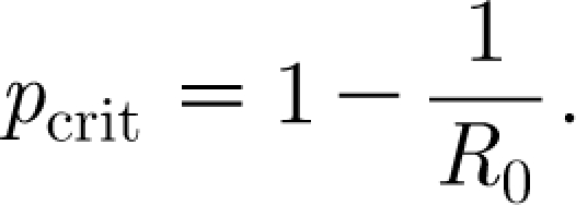
One of the most important insights achieved from the analysis of simple mathematical models is the concept of basic reproduction number R 0, defined as the average number of secondary cases generated by a ‘typical’ infectious case, throughout the infectious period, in a totally susceptible population. Its importance arises because it provides a link between mathematical models, actual epidemics and public health planning, which is relatively independent of other underlying details (Grassly & Fraser 2008). If one can calculate R 0 as a function of the underlying parameters, which characterize the mechanisms of transmission and the effects of public health interventions, then direct analytical insight is immediately gained into how these parameters relate to the intensity and magnitude of an ensuing epidemic. If this number is smaller than 1, the infectious agent is unable to sustain itself in the population; when it is bigger than 1, although random events could cause the extinction of the pathogen after a few cases, there is a positive probability for a large epidemic to take off. In addition to this threshold property, R 0 has a simple relationship with the critical vaccination coverage p crit, i.e. the fraction of the population that one needs to vaccinate in order to avoid a major outbreak,
 |
Despite its importance, for some models, other more explicit and sometimes more useful reproduction numbers can be defined (Becker & Dietz 1995, 1996; Ball et al. 1997; Becker & Starczak 1997; Ball & Neal 2002, 2008; Roberts & Heesterbeek 2003; Heesterbeek & Roberts 2007). As for R 0, their importance relies on the fact that they can summarize much of the information about the spread of the infection in a single number (Jansen et al. 2003), and, hopefully, they can provide insight into the effort required to stop the epidemic.
In this paper, we describe a model that is relevant for any infection that confers permanent immunity after recovery and for which the presence of clusters of individuals (e.g. households or schools/workplaces) is a key factor in determining its spread, in particular airborne infections such as severe acute respiratory syndrome (SARS), influenza, measles, chickenpox and so on.
More specifically, we describe an SIR model, i.e. a model where susceptible individuals (S) can be infected (I) and then become permanently immune after recovery (R), in a population partitioned into households and workplaces. We recall a threshold parameter R * first proposed by Ball & Neal (2002), and we define and discuss a new household-to-household reproduction number, called R H. The population is assumed to be large and attention is focused on the early phase of the epidemic, i.e. when the fraction of the population infected is still negligible.
Note that, except when otherwise stated, in the rest of this paper, we will not specify any particular model for the infection process, i.e. for the disease history of an infected individual and for the dynamics of their interaction with a susceptible one, since the results presented have a general form which does not depend on such level of detail. In particular, the presence or absence of a latent period (i.e. when individuals are infected but not yet infectious) will not affect the following discussion and, more generally, the concept of time will not be modelled explicitly.
However, we require two assumptions concerning the spread of the infection to be satisfied, which are as follows.
(i) The disease history of an infective does not depend on the identity of the individual who caused the infection; in other words, we assume that there is no correlation in biological infectiousness between infector and infectee (see §§2.2 and 5.3 of Diekmann & Heesterbeek 2000).
(ii) External conditions, such as seasonal variations or other social changes, that would affect the mixing patterns in the population or the interaction between individuals and the pathogen remain constant throughout the epidemic.
Such simplifying assumptions appear frequently (and often implicitly) in epidemiological modelling and are required here as sufficient conditions for the mathematical results presented in this paper to hold. Note, however, that they may be relaxed: assumption (ii) is mainly required since the quantities studied in this paper are treated as constant, although, in a realistic context, they can vary through time. A discussion of these is rather technical in nature and is reported in the electronic supplementary material.
The rest of this paper is organized as follows. Section 2 recalls some of the key features of models where the population is structured into households. Section 3 presents a model with households and workplaces, the main topic of this study, and contains a description of the model (§3.1), a definition of the new threshold parameter R H (§3.2) and how it relates to vaccination strategies targeted at randomly selected households (§3.3). Section 4 is then devoted to general comments and conclusions.
2. Households models
When interest is focused on directly transmitted infections, it is natural to assume that the household represents the most fundamental unit of transmission, followed by the workplace/school structure and then by local communities, towns, cities, etc. (Longini & Koopman 1982; Edmunds et al. 1997). Such an a priori assumption has been supported by complex microsimulations (Elveback et al. 1971, 1976) and has recently been confirmed more quantitatively from the behaviour of similar but larger and more robustly parametrized studies (Longini et al. 2004, 2005; Ferguson et al. 2005, 2006; Germann et al. 2006; Riley & Ferguson 2006). Moreover, the household is often the fundamental unit at which control policies are targeted, because of both practical reasons (people who want or are asked to limit their movements are more likely to stay at home than anywhere else) and structural reasons (decisions about action or compliance to control policies are usually taken by the family as a unit).
Therefore, in the attempt to model a more realistic social structure while still allowing for some analytical tractability, the first step is achieved by assuming that the population is partitioned into households and that homogeneous mixing within the household is superimposed on the homogeneous mixing (usually at a much smaller rate) occurring in the population at large (Ball et al. 1997).
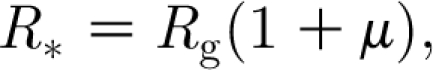
These so-called households models have been studied during the last 15 years (Becker & Dietz 1995; Ball et al. 1997, 2004), although the idea goes back to Bartoszynski (1972). The models are mathematically challenging—owing to the fact that, even in a large population and at the beginning of an epidemic, the infection process occurring in a household cannot be linearized since the size of the household is small and the local depletion of susceptibles cannot be ignored. Among many important results, the one that is relevant for this study is the definition of a reproduction number, denoted by R *, representing the average number of households infected by a typical infected household in a totally susceptible population (Ball et al. 1997; Wu et al. 2006; Fraser 2007). This reproduction number for households satisfies the usual threshold property: when R *>1, large epidemics can occur; when R *<1 no large epidemic can occur. Its analytical expression is of the form
 |
2.1 |
where R g represents the average number of infections generated by an infective outside their household and 1+μ represents the average size of an epidemic in a household, given by the sum of the primary case that imported the infection from outside (in a large population and at the beginning of the epidemic, multiple reintroductions are rare) and the average number of other cases μ. This average takes into account the fact that larger households are more likely to be infected than smaller ones. Note that the factorization of R * is a non-trivial result and depends on our model assumptions (see the electronic supplementary material or Ball et al. (1997) and Andersson & Britton (2000) for more details).
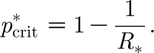
The basic reproduction number R 0 can still be defined in this model, although care needs to be taken in describing what a typical infectious case is. Some authors (e.g. Ball et al. 1997) consider a typical case as a randomly selected individual in a fully susceptible population. In this case, when R 0>1, the infection quickly spreads in the household of the initial case, but may still be unable to spread widely between households and may not result in a large epidemic, i.e. R 0 is not a useful threshold parameter. We personally prefer to maintain the threshold property of R 0, and we do so by letting the infection spread through the household of the first randomly selected case in the population and then defining a typical case by averaging across all the individuals infected in the household. Unfortunately, with such a definition, the nonlinearity induced by the quick depletion of susceptibles within the households makes R 0 analytically intractable, because the number of new cases generated by an infective varies according to how many susceptibles are still present in the household and is therefore difficult to compute. R * does not suffer from this problem since it refers to entire households (the complexity due to the local depletion of susceptibles is captured in μ) and the household-to-household infection process becomes linear in the limit of an infinite number of households and in the initial phase of the epidemic (Ball et al. 1997; Fraser 2007). As for R 0 in the homogeneously mixing case, R * is linked to a critical vaccination coverage by the formula
 |
2.2 |
In this case, however,  refers to households, i.e. it represents the fraction of randomly selected households that one needs to vaccinate in order to avoid large epidemics (Becker & Dietz 1995; Ball et al. 1997; Fraser 2007). Since vaccination strategies or other control policies such as quarantine and prophylactic treatment are more likely to be targeted to entire households than to randomly selected individuals (Becker & Dietz 1995; Becker & Utev 1998; Wu et al. 2006; Fraser 2007), R
* might, in some contexts, be a more useful parameter to estimate than R
0. Note, however, that vaccinating whole households, though administratively convenient, is not an optimal policy in terms of using a scarce vaccine (Ball et al. 1997). Other more efficient and practically viable strategies have been considered in House & Keeling (in press).
refers to households, i.e. it represents the fraction of randomly selected households that one needs to vaccinate in order to avoid large epidemics (Becker & Dietz 1995; Ball et al. 1997; Fraser 2007). Since vaccination strategies or other control policies such as quarantine and prophylactic treatment are more likely to be targeted to entire households than to randomly selected individuals (Becker & Dietz 1995; Becker & Utev 1998; Wu et al. 2006; Fraser 2007), R
* might, in some contexts, be a more useful parameter to estimate than R
0. Note, however, that vaccinating whole households, though administratively convenient, is not an optimal policy in terms of using a scarce vaccine (Ball et al. 1997). Other more efficient and practically viable strategies have been considered in House & Keeling (in press).
3. A model with households and workplaces
3.1. Model description
A possible generalization of the households model towards an even more realistic social structure is achieved when individuals belong to more than one type of mixing group and different groups are allowed to overlap (Ball & Neal 2002). Here, we consider one of the simplest examples of these overlapping groups models.
Consider a very large population and partition it in two different ways, into households and workplaces, so that each individual belongs to a household and a workplace. The concept of workplace is intended as the place where people spend most of their time out of home (e.g. actual workplaces, schools, other types of social groups and so on).
Assume furthermore that each individual living in a household selects their workplace randomly (i.e. the graph connecting households and workplaces is a bipartite random graph (Newman 2002); see the electronic supplementary material for a more detailed description). Although unrealistic, this assumption is mathematically convenient, as it allows for analytical results that do not depend on the details of the social structure.
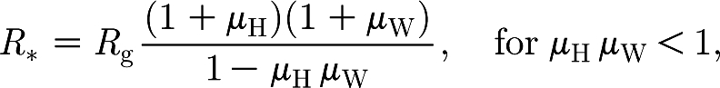
There are three possible types of infection: within the household; within the workplace (both considered local infections); or between an infectious individual and a randomly chosen susceptible in the population (global infections, usually at a small rate). A clump is defined as the set of individuals infected by chains of local infections (through household and workplace contacts). Each subsequent global infection from individuals in the clump gives rise to a new clump. Ball & Neal (2002) defined R * as the reproduction number for clumps, i.e. the average number of clumps infected by a typical clump in a totally susceptible population. The analytical expression for it (eqn (10) in Ball & Neal (2002), although in a different notation; see the electronic supplementary material for a derivation) is
 |
3.1 |
where R g is the average number of global infections generated by a single individual and μ H and μ W are the average sizes of a local epidemic in a household and a workplace, respectively (more exactly, in the household/workplace of a randomly chosen individual, since larger households are more likely to be infected). The local epidemics are started by a single initial case, which is not counted in the final size.
Note that, similarly to what happened for the households model of §2, the formula for R * contains two different factors and can be read as
Again, the factorization is non-trivial (see the electronic supplementary material).
The average size of a clump tends to infinity as μ H μ W tends to 1 from below, and therefore R *, although not formally defined, can be considered to be infinite when μ H μ W≥1.
R * satisfies the usual threshold property, i.e. large epidemics can occur only if R *>1. However, it has some limitations, which are as follows.
—
 can become infinite, since the average size of a clump can become infinite (Ball & Neal 2002) and the condition for it to happen (μ
H
μ
W≥1) is likely to occur in practice (it is sufficient to think about the large epidemics that may occur in schools).
can become infinite, since the average size of a clump can become infinite (Ball & Neal 2002) and the condition for it to happen (μ
H
μ
W≥1) is likely to occur in practice (it is sufficient to think about the large epidemics that may occur in schools).— The time required for a clump to form increases as μ H μ W tends to 1 and becomes quickly comparable with the time of the whole epidemic.
— A critical vaccination coverage obtained from this parameter will refer to clumps, but a clump is a random set of individuals and cannot be identified and vaccinated beforehand.
3.2. A new threshold parameter for the households–workplaces model
Since a vaccine not only can but is also likely to be delivered to entire households (Becker & Dietz 1995; Becker & Utev 1998; Wu et al. 2006; Fraser 2007), a reproduction number for households is more relevant from a practical point of view. Analogously, it may also be more directly related to other forms of intervention targeted at households, such as households quarantine and prophylaxis (Fraser 2007). Therefore, we define R H as the average number of households infected by a typical household in a totally susceptible population. Now, the infection can exit from a household following two routes: via a global infection or via a workplace infection, i.e. when an infected individual in the household triggers an epidemic in their workplace and all those ultimately infected are primary cases in new households.
Following Diekmann & Heesterbeek (2000), we define R ij, for i, j∈{L,G}, as the average number of households infected via a type-i infection by a household that has been infected through a type-j infection. The letters L and G refer to local workplace infections and global infections, respectively.
It is convenient to attribute all the final cases of a local epidemic to the individual who started it. In this way, when a household is infected locally (j=L), the primary case does not play any active role in the workplace epidemic that caused their infection. Instead, this primary case starts a household epidemic and generates an average of μ H secondary cases. Each of them belongs to a different workplace and starts a workplace epidemic with average final size μ W, causing a total average of μ H μ W new primary cases, each one in a different household. Therefore, R LL=μ H μ W (figure 1). Furthermore, in the household under consideration, each infective (including the primary case) also generates R g new infectives outside, and each of these new infectives is a primary case in a new household. Therefore, R GL=R g(1+μ H) (figure 1).
Figure 1.

Graphical description of the quantities (a) R GG, (b) R GL, (c) R LG and (d) R LL, used in the main text to construct the household-to-household next-generation matrix, from which the threshold parameter R H is then computed. In this case, R g=2, μ H=2 and μ W=1. Straight arrows represent local infections within households (rectangles) or workplaces (ellipses), arc arrows represent global infections. The black circle represents the household primary case and the grey circle indicates all the other infected cases in the household (attributed to, although not necessarily caused directly by, the primary case).
The same arguments apply when the household is infected globally (j=G), except for the fact that the primary case can now trigger an epidemic in their workplace as well as in the household. Therefore, R LG=μ W(1+μ H) and R GG=R g(1+μ H).
The proper way of averaging the two types of household infections is to consider the next-generation matrix (see Diekmann & Heesterbeek 2000),
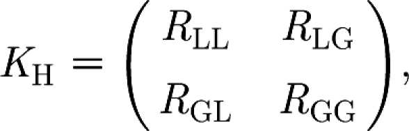 |
and its dominant eigenvalue,
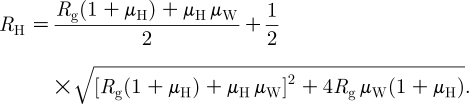 |
3.2 |
R H satisfies the usual threshold property, i.e. large epidemics can occur only if R H>1, and is related to R * according to the following.
Theorem 3.1. —
For all non-negative values of R g, μ H and μ W,
—
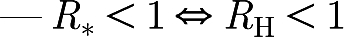
—
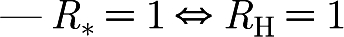
—
i.e. R* and R H share the same threshold at 1 and are consistent in their threshold property.
Apart from their behaviour around 1, the relationship between R * and R H is non-trivial. In particular, it is possible that, for some changes of R g, μ H and μ W, one of the two reproduction numbers increases while the other decreases (see the electronic supplementary material).
Following similar arguments, a workplace-to-workplace reproduction number R W can also be defined. The analytical formula for R W is obtained by swapping μ H and μ W in the formula for R H. R W too satisfies the threshold property and, although non-trivially related to R H and R *, shares the same threshold at 1 with them. In the rest of this paper, we focus mostly on R H, although all the comments also hold for R W when workplaces are considered instead of households.
R H overcomes some of the limitations of R * presented above:
(i) R H can never become infinite,
(ii) the time a household requires to infect other households is limited and usually much shorter than the time of the whole epidemic, and
(iii) R H can be related to a critical vaccination coverage
 for households.
3.3. Vaccination
Unfortunately, the relationship between R
H and  is not as simple as the usual one (see equation (2.2)), because of the non-trivial dependence of the final size of a local epidemic in a workplace on the initial number of susceptibles available. However, we formally proved (see the electronic supplementary material) the following.
Theorem 3.2. —
Consider an epidemic in a closed and homogeneously mixing population with a single initial infective and n initial susceptibles. Let μ be the average final size (excluding the initial case) of an epidemic spreading in it. Let a random number m<n of initial susceptibles be vaccinated (totally immune) and define P=m/n. Let
and q=1−p, and define μV to be the average final size of an epidemic after vaccination. Then, μV≤qμ.
Remark 3.3. —
Two possible special cases of theorem 3.2 are obtained when
a fixed number m out of the n susceptibles is vaccinated and
each susceptible is vaccinated independently with probability p; in this case, m∼Bin(n,p).
Assume, for the time being, that all households have the same size. Then, theorem 3.2 can be applied to workplaces since, when a fraction p (or a random fraction P with average p) of the households is selected and all the members are vaccinated effectively, our assumption of random connections between households and workplaces implies that individuals in workplaces are vaccinated independently of each other and with probability p (case (ii)). Therefore,
 |
Since after the vaccination μ
H is not modified and R
g is reduced to  , a direct consequence is the following.
Corollary 3.4. —
The fraction
of households (all of the same size) that one needs to vaccinate in order to control the epidemic satisfies
3.3
Corollary 3.4 states that the effect of vaccination on R
H is ‘more than linear’, i.e. vaccinating a proportion of households equal to 1−1/R
H will reduce the value of  at least to 1 if not below. This means that the value 1−1/R
H represents a secure vaccination coverage (in the terminology of Ball et al. (2004)). Figure 2 shows that vaccination of a proportion 1−1/R
H of households is just sufficient to reduce R
H below 1 when infectivity in workplaces is very low or very high, but that for intermediate values of such infectivity less effort would be required, although an exact quantification can only be assessed numerically and depends on model assumptions about the individuals' infectivity. Numerical values in figure 2 are obtained using the so-called standard SIR model defined in Ball (1983; see also Ball (1986) and Andersson & Britton (2000) and the electronic supplementary material).
at least to 1 if not below. This means that the value 1−1/R
H represents a secure vaccination coverage (in the terminology of Ball et al. (2004)). Figure 2 shows that vaccination of a proportion 1−1/R
H of households is just sufficient to reduce R
H below 1 when infectivity in workplaces is very low or very high, but that for intermediate values of such infectivity less effort would be required, although an exact quantification can only be assessed numerically and depends on model assumptions about the individuals' infectivity. Numerical values in figure 2 are obtained using the so-called standard SIR model defined in Ball (1983; see also Ball (1986) and Andersson & Britton (2000) and the electronic supplementary material).
Figure 2.

Values of  , i.e. the household-to-household reproduction number after the vaccination of a proportion 1−1/R
H of randomly selected households. The curves correspond (from bottom to top) to R
g=0.2, 0.5, 1, 2, 4, 8 and 15. Numerical values are obtained by fixing μ
H=2 (other values lead to qualitatively similar results), and assuming that all workplaces have size n=6 and that the epidemic in a workplace spreads according to the standard SIR model defined in Ball (1983; see also Ball (1986) and Andersson & Britton (2000) and the electronic supplementary material), with infectious period of fixed length and individual-to-individual infection rate β/(n−1). The results are similar for other values of n, thus showing that it can be extended to a non-singular workplace size distribution (the value of μ
H already takes into account variable sizes for households). The model is equivalent to a Reed–Frost model with individual-to-individual escaping probability π=exp(−β/(n−1)) (see Ludwig (1975) and Pellis et al. (2008) and the electronic supplementary material). Other model assumptions (other distributions for the length of the infectious periods in the standard SIR model or other models with time-varying infection rates) lead to qualitatively similar results.
, i.e. the household-to-household reproduction number after the vaccination of a proportion 1−1/R
H of randomly selected households. The curves correspond (from bottom to top) to R
g=0.2, 0.5, 1, 2, 4, 8 and 15. Numerical values are obtained by fixing μ
H=2 (other values lead to qualitatively similar results), and assuming that all workplaces have size n=6 and that the epidemic in a workplace spreads according to the standard SIR model defined in Ball (1983; see also Ball (1986) and Andersson & Britton (2000) and the electronic supplementary material), with infectious period of fixed length and individual-to-individual infection rate β/(n−1). The results are similar for other values of n, thus showing that it can be extended to a non-singular workplace size distribution (the value of μ
H already takes into account variable sizes for households). The model is equivalent to a Reed–Frost model with individual-to-individual escaping probability π=exp(−β/(n−1)) (see Ludwig (1975) and Pellis et al. (2008) and the electronic supplementary material). Other model assumptions (other distributions for the length of the infectious periods in the standard SIR model or other models with time-varying infection rates) lead to qualitatively similar results.
The same considerations apply when households and workplaces have variable size distributions, when households are selected at random, i.e. independently of their size. However, when sizes vary, other strategies of household selection (e.g. vaccination of the largest households or the households of randomly selected individuals) can be considered and in general perform better. A more detailed discussion about such selection criteria is reported in the electronic supplementary material.
The main reason for adding the workplaces to the household structure, apart from making the model slightly more realistic, is to study the effect of their closure on the spread of the epidemic. This can be simulated by setting μ W=0 in both the formulae of R * and R H, and, in both cases, as expected, the formula for R * of the households model of §2 is recovered. Note, however, that the explicit presence of workplaces in the present model allows the effects of their closure to be disentangled from other forms of social distancing. In fact, should the individual's behaviour remain unchanged before and after the implementation of this control policy, the value of the other parameters R g and μ H in the model would remain constant, while the parameter R g in the households model would actually be reduced (in a non-trivial fashion) because it takes into account any form of between-household transmission, including that occurring at work.
4. Discussion and conclusions
We have considered a model (first proposed in Ball & Neal 2002) for a population partitioned into households and workplaces, we have shown that more than one reproduction number with a clear epidemiological interpretation can be defined and, in particular, we have presented a new household-to-household reproduction number R H (equation (3.2)).
A construction similar to that leading to R H has been adopted independently in Ball & Neal (2008), although with rather different motivation and derivation. In Ball & Neal (2008), superimposed to global infections, local infections occur between individuals (and not households) on a random contact network with specified degree distribution. In the infinite population limit, local saturation can be neglected and therefore only direct infections are attributed to each infective; for this reason, the threshold parameter obtained is actually the basic reproduction number R 0. In our model, the network representing local contacts consists of fully connected sub-graphs (households and workplaces), joint by single nodes, and local infections between households spread through workplace epidemics, where the nonlinearity induced by the local saturation is bypassed by referring all cases in a workplace epidemic to the primary case.
We have shown how R H overcomes some of the limitations from which the clump-to-clump reproduction number R * suffers (Ball & Neal 2002). In particular, it can never become infinite, and it is therefore always informative about how much effort should be put into controlling the epidemic. As a numerical example, let (R g, μ H, μ W)=(1/3, 1, 1); while R *=∞, R H=2. We therefore know that the household-to-household transmission must be reduced by a factor of 2. By keeping fixed both μ H (i.e. we act only on between-household transmission) and R g (e.g. because we think we cannot easily control it quantitatively), we find (now R H changes monotonically with μ W) that μ W needs to be reduced from 1 to 0.2 to achieve control. Of course, the same result can be obtained from R *, since it shares the same threshold with R H, but requiring a reduction of R * from ∞ to 1 is less informative from a practical point of view.
Another remark in support of R H is that a selected household requires a limited time to infect other households. Therefore, in a reasonably large but finite population, it is often possible to ignore the depletion of susceptibles for long enough to be able to observe a number of household-to-household infections, which is sufficiently large for the law of large numbers to be invoked, i.e. for having the epidemic behaviour mainly driven by the household-to-household reproduction number (an average value). On the contrary, already when μ H μ W is smaller than but close to 1, the time required for a clump to form may be so long that any realistic population size could be too small to make the exponential phase long enough to observe clumps reaching the end of their infectious period before the depletion of susceptibles in the population starts having a major role in the epidemic dynamics.
We have formally proved an inequality (equation (3.3)) for the critical vaccination coverage for households, which provides an upper bound for the effort needed to safely contain the epidemic when vaccination is targeted at randomly selected households instead of randomly selected individuals; such vaccination policy, although not optimal (Becker & Starczak 1997; Ball & Lyne 2002; Ball et al. 2004), is likely to be the one adopted in most practical cases (Becker & Utev 1998; Fraser 2007). Note that, if the assumption of random connections between households and workplaces is not met, the inequality (3.3), although not strict, remains valid and therefore the vaccination of a proportion of randomly selected households equal to 1−1/R H still guaranties infection extinction.
We also commented on the fact that the same argument that leads to equation (3.2) for R H can be used to derive a similar reproduction number R W for workplaces. All the results valid for R H are also valid for R W when the roles of households and workplaces are exchanged. We have focused mainly on R H since the household is often a more natural target for control policies than a workplace, because it is more clearly identifiable, because of the often higher internal transmission coefficient or because most of the population has a household to live in. In some contexts, however, R W may be more relevant than R H, for example when vaccination is delivered to children in schools or some other forms of controls targeted at workplaces are studied.
The presence of workplaces in addition to households allows us to study the effect of the social distancing achieved when people stop going to work. Such an action is surely a draconian measure and is not likely to be implemented because of its economical implications. However, school closure is not only feasible but also more likely to occur under conditions of particular stress for the health care system and, as a side effect, it may force many workers to remain at home with their children.
It is reasonable to assume that school or workplace closure has an effect on other routes of transmission, since individuals not at work spend their time elsewhere. In this case, it may well happen that a reduction of some parameters (e.g. R g and μ W) is accompanied by an increase in others (e.g. μ H if, for example, more time is spent at home). These types of change in the parameter set can result in different reproduction numbers changing in different directions (see the electronic supplementary material). Therefore, their effect may be read differently by the two reproduction numbers R * and R H, and we argue that the information provided by both parameters should be taken into account and compared.
Other forms of intervention, especially those based on real-time reaction to detected or suspected cases, are more difficult to study, since they are highly dependent on the time delays between infection, detection of a case and policy implementation. This requires a detailed specification of the dynamics of the individual-to-individual infection process, which has not been modelled in this paper.
The choice of not modelling the dynamics of the infectious-to-susceptible interaction has the clear advantage that the results of this paper hold quite generally. As a drawback, it makes the quantities in the formulae for the reproduction numbers less easily related to more fundamental ingredients (such as infectivity, duration of infectiousness and so on) and therefore more difficult to find knowledge about. In particular, while μ H and μ W could be in principle estimated from data on where infected cases live and work, estimation of R g may be more difficult.
Our approach presents other limitations. First of all, we assumed that each individual selects their workplace randomly, thus giving rise to a social structure that can be described as a bipartite random network. Such a condition is clearly not met in a real society, because there is a spatial component that cannot be ignored (e.g. children going to school close to home, adults trying to find a job not too distant from where they live) and some forms of social aggregation (e.g. work colleagues deciding to register their children to the same school; cultural, religious or political affinities and so on). Relaxing this hypothesis can probably be achieved only by using individual-based simulations and is currently under investigation by the authors. However, this random network assumption provides the worst possible scenario, since it minimizes the chance that the infection re-enters in the same infected household or workplace, an event that would slow down the epidemic and reduce its final size.
A second limitation is the idealization of the concept of workplace, assumed to be a place where individuals spend most of their time while out of home; in practice, it is often unclear who should be considered as sharing a workplace with whom. However, the same definition problems arise in quantifying the effects of most of the social distancing control measures implemented during an infection outbreak.
Many other interesting issues should be further explored: first, gaining a clear understanding of the differences between a households–workplaces model, as described in this paper, and other structured population models where the local saturation of susceptibles is not taken into account (e.g. Roberts 2004, 2007; Aldis 2005) or is taken into account only for the within-household transmission (e.g. in Becker et al. 2005); second, investigating the benefits of a further distinction between schools and workplaces, motivated by a difference in size distributions, transmission parameters, contact rates and other characteristics of the individuals (adult/child), the economic implications of their closure, as well as realistic feasibility of parameter estimation in the two environments (Cauchemez et al. 2008); third, exploring how important the presence of workplaces is, in addition to the household structure, in correctly estimating the target of the critical vaccination coverage, as in Becker & Utev (1998) for the comparison between a households model and a model with homogeneous mixing. Furthermore, in order to assess the impact that school and workplace closure might have in an emerging outbreak situation, extensive effort needs to be focused on quick and robust methods for the estimation of the changes in global and household transmission that are likely to occur when the control policy is implemented. Some a priori analysis could be carried out by assuming that the social behaviour in such conditions is similar to what is obtained during school holidays, as in Cauchemez et al. (2008). However, human behaviour under considerably stressful conditions, such as during an emerging outbreak, is difficult to predict and may turn out to be substantially different from what can be observed during normal holiday time. For this reason, real-time estimation methods remain invaluable tools and much effort should be spent in identifying which data need to be collected and how.
Acknowledgments
We gratefully acknowledge the MRC Centre for Outbreak Analysis and Modelling and the Institute for Mathematical Sciences, Imperial College London, for funding; we also thank Prof. Frank G. Ball for having provided the basic ideas for the proof of theorem 3.2 and the anonymous referees for having considerably improved the quality of the manuscript.
References
- Aldis G. K.2005An integral equation model for the control of a smallpox outbreak. Math. Biosci. 195, 1. 10.1016/j.mbs.2005.01.006 [DOI] [PubMed] [Google Scholar]
- Anderson R. M., May R. M. 1991. Infectious diseases of humans: dynamics and control. Oxford, UK:Oxford University Press [Google Scholar]
- Andersson H., Britton T. 2000. Stochastic epidemic models and their statistical analysis. In Lecture Notes in Statistics vol. 151New York, NY; London, UK:Springer [Google Scholar]
- Bailey N. T. J. 1975. The mathematical theory of infectious diseases and its applications 2nd edn.London, UK:Griffin [Google Scholar]
- Ball F. G.1983The threshold behaviour of epidemic models. J. Appl. Probab. 20, 227. 10.2307/3213797 [DOI] [Google Scholar]
- Ball F. G.1986A unified approach to the distribution of total size and total area under the trajectory of infectives in epidemic models. Adv. Appl. Probab. 18, 289–310. 10.2307/1427301 [DOI] [Google Scholar]
- Ball F. G., Lyne O. D.2002Optimal vaccination policies for stochastic epidemics among a population of households. Math. Biosci. 177, 333–354. 10.1016/S0025-5564(01)00095-5 [DOI] [PubMed] [Google Scholar]
- Ball F. G., Neal P.2002A general model for stochastic SIR epidemics with two levels of mixing. Math. Biosci. 180, 73–102. 10.1016/S0025-5564(02)00125-6 [DOI] [PubMed] [Google Scholar]
- Ball F. G., Neal P.2008Network epidemic models with two levels of mixing. Math. Biosci. 212, 69–87. 10.1016/j.mbs.2008.01.001 [DOI] [PubMed] [Google Scholar]
- Ball F. G., Mollison D., Scalia-Tomba G.1997Epidemics with two levels of mixing. Ann. Appl. Probab. 7, 46–89. 10.1214/aoap/1034625252 [DOI] [Google Scholar]
- Ball F. G., Britton T., Lyne O. D.2004Stochastic multitype epidemics in a community of households: estimation of threshold parameter R* and secure vaccination coverage. Biometrika. 91, 345–362. 10.1093/biomet/91.2.345 [DOI] [PubMed] [Google Scholar]
- Bartoszynski R.1972On a certain model of an epidemic. Appl. Math. 13, 139–151. [Google Scholar]
- Becker N. G., Dietz K.1995The effect of household distribution on transmission and control of highly infectious diseases. Math. Biosci. 127, 207–219. 10.1016/0025-5564(94)00055-5 [DOI] [PubMed] [Google Scholar]
- Becker N. G., Dietz K. 1996. Reproduction numbers and critical immunity levels for epidemics in a community of households In Athens Conf. on Applied Probability and Time Series, Volume I: Applied Probability (eds Heyde C. C., Prohorov Yu. V., Pyke R., Rachev S. T. Lecture Notes in Statistics, no. 114, p. 267 Berlin, Germany: Springer [Google Scholar]
- Becker N. G., Starczak D. N.1997Optimal vaccination strategies for a community of households. Math. Biosci. 139, 117. 10.1016/S0025-5564(96)00139-3 [DOI] [PubMed] [Google Scholar]
- Becker N. G., Utev S.1998The effect of community structure on the immunity coverage required to prevent epidemics. Math. Biosci. 147, 23–39. 10.1016/S0025-5564(97)00079-5 [DOI] [PubMed] [Google Scholar]
- Becker N. G., Bahrampour A., Dietz K.1995Threshold parameters for epidemics in different community settings. Math. Biosci. 129, 189–208. 10.1016/0025-5564(94)00061-4 [DOI] [PubMed] [Google Scholar]
- Becker N. G., Glass K., Li Z., Aldis G. K.2005Controlling emerging infectious diseases like SARS. Math. Biosci. 193, 205–221. 10.1016/j.mbs.2004.07.006 [DOI] [PubMed] [Google Scholar]
- Cauchemez S., Valleron A. J., Boelle P. Y., Flahault A., Ferguson N. M.2008Estimating the impact of school closure on influenza transmission from Sentinel data. Nature. 452, 750–754. 10.1038/nature06732 [DOI] [PubMed] [Google Scholar]
- Diekmann O., Heesterbeek J. A. P. 2000. Mathematical epidemiology of infectious diseases: model building, analysis and interpretation.. In Wiley Series in Mathematical and Computational Biology Chichester, UK:Wiley [Google Scholar]
- Edmunds W. J., O'Callaghan C. J., Nokes D. J.1997Who mixes with whom? A method to determine the contact patterns of adults that may lead to the spread of airborne infections. Proc. R. Soc. B. 264, 949–957. 10.1098/rspb.1997.0131 [DOI] [PMC free article] [PubMed] [Google Scholar]
- Elveback L. R., Ackerman E., Gatewood L., Fox J. P.1971Stochastic two-agent epidemic simulation models for a community of families. Am. J. Epidemiol. 93, 267–280. [DOI] [PubMed] [Google Scholar]
- Elveback L. R., Fox J. P., Ackerman E., Langworthy A., Boyd M., Gatewood L.1976An influenza simulation model for immunization studies. Am. J. Epidemiol. 103, 152–165. [DOI] [PubMed] [Google Scholar]
- Ferguson N. M., Keeling M. J., Edmunds W. J., Gani R., Grenfell B. T., Anderson R. M., Leach S.2003Planning for smallpox outbreaks. Nature. 425, 681–685. 10.1038/nature02007 [DOI] [PMC free article] [PubMed] [Google Scholar]
- Ferguson N. M., Cummings D. A. T., Cauchemez S., Fraser C., Riley S., Meeyai A., Iamsirithaworn S., Burke D. S.2005Strategies for containing an emerging influenza pandemic in Southeast Asia. Nature. 437, 209–214. 10.1038/nature04017 [DOI] [PubMed] [Google Scholar]
- Ferguson N. M., Cummings D. A. T., Fraser C., Cajka J. C., Cooley P. C., Burke D. S.2006Strategies for mitigating an influenza pandemic. Nature. 442, 448. 10.1038/nature04795 [DOI] [PMC free article] [PubMed] [Google Scholar]
- Fraser C.2007Estimating individual and household reproduction numbers in an emerging epidemic. PLoS ONE. 2, e758. 10.1371/journal.pone.0000758 [DOI] [PMC free article] [PubMed] [Google Scholar]
- Germann T. C., Timothy C., Kadau K., Longini I. M., Macken C. A.2006Mitigation strategies for pandemic influenza in the United States. Proc. Natl Acad. Sci. USA. 103, 5935–5940. 10.1073/pnas.0601266103 [DOI] [PMC free article] [PubMed] [Google Scholar]
- Grassly N. C., Fraser C.2008Mathematical models of infectious disease transmission. Nat. Rev. Microbiol. 6, 477–487. 10.1038/nrmicro1845 [DOI] [PMC free article] [PubMed] [Google Scholar]
- Heesterbeek J. A. P., Roberts M. G. 2007. The type-reproduction number T in models for infectious disease control. Math. Biosci. 206, 3–10 10.1016/j.mbs.2004.10.013 [DOI] [PubMed] [Google Scholar]
- Hethcote H. W.2000The mathematics of infectious diseases. SIAM Rev. 42, 599. 10.1137/S0036144500371907 [DOI] [Google Scholar]
- House T., Keeling M. J.Household structure and infectious disease transmission. Epidemiol. Infect In press 10.1017/S0950268808001416 [DOI] [PMC free article] [PubMed] [Google Scholar]
- Jansen V. A. A., Stollenwerk N., Jensen H. J., Ramsay M. E., Edmunds W. J., Rhodes C. J.2003Measles outbreaks in a population with declining vaccine uptake. Science. 301, 804. 10.1126/science.1086726 [DOI] [PubMed] [Google Scholar]
- Kermack W. O., McKendrick A. G.1927A contribution to the mathematical theory of epidemics. Proc. R. Soc. A. 115, 700–721. 10.1098/rspa.1927.0118 [DOI] [Google Scholar]
- Longini I. M., Koopman J. S.1982Household and community transmission parameters from final distributions of infections in households. Biometrics. 38, 115–126. 10.2307/2530294 [DOI] [PubMed] [Google Scholar]
- Longini I. M., Halloran M. E., Nizam A., Yang Y.2004Containing pandemic influenza with antiviral agents. Am. J. Epidemiol. 159, 623. 10.1093/aje/kwh092 [DOI] [PubMed] [Google Scholar]
- Longini I. M., Nizam A., Xu S., Ungchusak K., Hanshaoworakul W., Cummings D. A. T., Halloran M. E.2005Containing pandemic influenza at the source. Science. 309, 1083–1087. 10.1126/science.1115717 [DOI] [PubMed] [Google Scholar]
- Ludwig D.1975Final size distributions for epidemics. Math. Biosci. 23, 33. 10.1016/0025-5564(75)90119-4 [DOI] [Google Scholar]
- Newman M. E. J.2002Spread of epidemic disease on networks. Phys. Rev. E. 66, 016 128. 10.1103/PhysRevE.66.016128 [DOI] [PubMed] [Google Scholar]
- Pellis L., Ferguson N. M., Fraser C.2008The relationship between real-time and discrete-generation models of epidemic spread. Math. Biosci. 216, 63–70. 10.1016/j.mbs.2008.08.009 [DOI] [PubMed] [Google Scholar]
- Riley S., Ferguson N. M.2006Smallpox transmission and control: spatial dynamics in Great Britain. Proc. Natl Acad. Sci. USA. 103, 12 637–12 642. 10.1073/pnas.0510873103 [DOI] [PMC free article] [PubMed] [Google Scholar]
- Roberts M. G.2004Modelling strategies for minimizing the impact of an imported exotic infection. Proc. R. Soc. B. 271, 2411–2415. 10.1098/rspb.2004.2865 [DOI] [PMC free article] [PubMed] [Google Scholar]
- Roberts M. G.2007A model for the spread and control of pandemic influenza in an isolated geographical region. J. R. Soc. Interface. 4, 325–330. 10.1098/rsif.2006.0176 [DOI] [PMC free article] [PubMed] [Google Scholar]
- Roberts M. G., Heesterbeek J. A. P.2003A new method for estimating the effort required to control an infectious disease. Proc. R. Soc. B. 270, 1359–1364. 10.1098/rspb.2003.2339 [DOI] [PMC free article] [PubMed] [Google Scholar]
- Wu J. T., Riley S., Fraser C., Leung G. M.2006Reducing the impact of the next influenza pandemic using household-based public health interventions. PLoS Med. 3, 1532–1540. 10.1371/journal.pmed.0030361 [DOI] [PMC free article] [PubMed] [Google Scholar]