Abstract
In this work singular value decomposition (SVD) techniques are used to investigate how the use of low energy photons and multiple energy windows affects the noise properties of Tc-99m SPECT imaging. We have previously shown that, when modeling scatter in the projector and backprojector of iterative reconstruction algorithms, simultaneous reconstruction from multiple energy window data can result in very different noise characteristics. Further, the properties depend upon the width and number of energy windows used. To investigate this further, we have generated photon transport matrices using models for scatter, an elliptical phantom containing cold rods of various sizes, and a number of multiple energy window acquisition schemes. Transfer matrices were also generated for the cases of perfect scatter rejection and ideal scatter subtraction. The matrices were decomposed using SVD, and signal power and projection space variance spectra were computed using the basis formed by the left singular vectors. Results indicate very different noise levels for the various energy window combinations. The perfect scatter rejection case resulted in the lowest variance spectrum, and reconstruction-based scatter compensation performed better than the scatter subtraction case. When including lower energy photons in reconstruction-based scatter compensation, using a series of multiple energy windows outperformed a single large energy window. One multiple window combination is presented which achieves a lower variance spectrum than the standard 20% energy window, indicating the potential for using low energy photons to improve the noise characteristics of SPECT images.
I. INTRODUCTION
The contamination of measured data in single photon emission computed tomography (SPECT) by scattered photons is often considered a degrading factor, causing inaccurate quantitation and loss of contrast in reconstructed images. For this reason, the estimated scatter component of the measured data is often subtracted [1–5]. However, such subtraction-based methods generally result in an accompanying increase in noise. Reconstruction-based scatter compensation (RBSC) [6,7] is a technique in which the scatter response function is modeled during the reconstruction. In effect, RBSC attempts to map scattered photons back to their point of origin. Since all acquired counts are used, RBSC is not subject to noise amplification.
In the past, RBSC has been applied to photopeak energy window projection data. However, the scatter response function (SRF) for Tc-99m imaging contains a peaked component even at energies well below the 140 kev emission peak. This indicates that low energy windows may contain some useful spatial information. The underlying premise of this work is that, by including low energy photons and modeling the scatter response function in the reconstruction, this information can be used to improve the noise characteristics of SPECT images.
In previous research we used the maximum-likelihood expectation-maximization (ML-EM) algorithm to reconstruct projection data spanning a wide energy range [8,9]. The SRF was modeled in the projector and backprojector, and reconstructions were performed for a variety of energy window combinations, each leading to different noise levels in the reconstructed images. This motivated us to investigate methods for optimizing the energy window combinations.
Because the choices of reconstruction algorithm and degree of regularization are task-dependent, we have chosen to use singular value decomposition (SVD) [10, 11] as a tool for analyzing noise propagation in SPECT. In the past Smith et al [12] investigated using SVD as a method for performing generalized matrix inverse (GMI) reconstructions, and more recently SVD has been used for both image reconstruction [13,14] and as a tool for investigating sampling requirements [15,16]. In this paper we use SVD as a tool to investigate the invertibility and inherent noise properties of a SPECT system for different multiple energy window acquisition schemes. A series of GMI reconstructions are also presented to help the reader assess the value of the SVD analysis methods, but we emphasize the usefulness of SVD as an analysis tool, not as a reconstruction method. Currently, iterative algorithms are more practical than using SVD for reconstructing images.
The SVD of the system matrix provides fundamental information about the invertibility and propagation of noise in a linear system. In order to use this information, we have developed metrics summarizing the propagation of noise which are a function of the degree of regularization of the GMI reconstruction (i.e., the point at which the singular value spectrum is truncated). Thus, these metrics may be useful to predict the behavior for a wide range of regularizations.
The metrics are first applied to several conventional strategies for handling scatter for data acquired in a 20% wide photopeak energy window centered on the emission peak. The analysis is then extended to RBSC methods which include lower energy photons acquired in both single and multiple energy windows. In this way the methods which model scatter are compared with conventional strategies, and the effects of including low energy scattered photons are assessed.
II. THEORY
A. Singular Value Decomposition
The basics of SVD are only briefly discussed here, and the reader should consult references such as [10–12] for further information. The projection image formation process in SPECT may be written in matrix-vector form as:
| (1) |
where,
Each projection datum is related to the activity distribution by a linear equation, hence eq. (1) describes a linear system of equations. The problem of reconstruction is to recover an estimate of the image, ỹ, from a measurement of the projections, p̃ (see [12] for a discussion of GMI reconstruction methods using SVD).
The SVD of the transfer matrix F can be written:
| (2) |
where,
The columns of U and V form orthonormal bases for the projection and image spaces, respectively. They represent changes to coordinate systems for which the corresponding transfer matrix (S) is diagonal.
The diagonal elements of S are known as the singular values and are usually arranged in descending order. If any of the singular values are zero, the problem is singular and cannot be inverted exactly. The singular vectors corresponding to the zero singular values form a basis for the null space, and represent information which is irretrievably lost by the projection operation. If no singular values are zero but some are very small, the solution is sensitive to small perturbations in the data (e.g. noise), and the problem is referred to as being ill-conditioned.
The SVD of F can be used to obtain the generalized matrix inverse reconstructed image as shown below:
| (3) |
where Sinv indicates the pseudo-inverse of S, including any regularization such as zeroing small singular values. If no regularization is applied, eq. (3) provides the least-squares solution to eq. (1). A better approach is to include statistical weights to obtain the weighted least-squares solution. However, this requires a separate SVD for each count level and source distribution. In this study we limit ourselves to the SVD of the transfer matrix and the least-squares solution.
B. Definition of Power Spectra
Traditionally, signal and noise power spectra have been calculated using the Fourier basis: the power spectrum of a process is the Fourier transform of its autocorrelation [17–19]. Since SPECT is count limited, the noise power is relatively high and dominates some components of the image. For this reason, reconstructed images are usually regularized by suppressing components of the image for which the noise power is expected to be higher than the signal power. This regularization is often achieved by the use of linear filters or by stopping iterative reconstructions at some point before the solution is reached. If the regularization scheme is a function of the Fourier components, comparisons of Fourier-based power spectra are easily obtained for all degrees of regularization. If this is not the case, e.g. when using stopping rules with iterative reconstruction algorithms, results using Fourier-based power spectra may be very regularization dependent. Another disadvantage of using the Fourier-based noise power spectrum is that it assumes the noise is a stationary processes, which is not the case in SPECT.
In this paper we use the singular vector basis obtained from the SVD of the system transfer matrix to express the signal power spectrum and a relative of the noise power spectrum, which we term the variance spectrum. The definitions of these spectra are given in detail below. Since images reconstructed using SVD are usually regularized by truncating or rolling-off the singular value spectrum at some point, these spectra are in one-to-one correspondence with the degree of regularization. Thus they provide information for a wide range of regularizations. For similar information to be obtained from iteratively reconstructed images, signal and noise power spectra would have to be calculated at each iteration.
The results based on the comparison of power spectra as defined in this paper are applicable to any linear regularization scheme. Since many iterative reconstruction algorithms in effect attempt to invert the system transfer matrix, it is possible the results based on SVD will correlate with iterative reconstructions as well. This hypothesis will be addressed in future research.
We define the measured signal power, MSPRSV (with superscript indicating the right singular vector basis has been used), to be the diagonal elements of the autocorrelation of the mean (noise-free) GMI reconstructed image components as expressed using the right singular vector basis:
| (4) |
where the angled brackets indicate the expectation value. We have used S−1 to indicate the inverse of the diagonal matrix of singular values. If any of the singular values are zero, their inverse should also be set to zero, not ∞ so that the reconstructed image contains no null components. The expectation is trivial since there are no random variables in the expression, and it reduces to:
| (5) |
The ith element of MSPRSV is simply the signal power of the image component recovered by including the ith singular value in the GMI reconstruction. For a quantitatively accurate reconstruction, MSPRSV will differ from the true signal power of the noise-free image only if (1) the problem is singular, in which case the measured signal power will be zero for all null image components; or (2) the noise-free projection data are not consistent with the models used for the transfer matrix.
Analogous to the signal power spectrum, the variance spectrum (VARRSV) is defined to be the diagonal elements of the autocorrelation of the noise in the GMI reconstructed image as expressed in the right singular vector basis:
| (6) |
where ñ represents the vector of noise in the estimate of the projections (p̃ = p̄ + ñ). The autocorrelation of the noise in the projections is the same as the autocovariance of the projections, and for Poisson statistics the variance equals the mean. The noise in the projections is also independent, and a few simple steps yields a working expression for the variance spectrum:
| (7) |
The ith element of VARRSV is simply the expected variance of the image component which is recovered by including the ith singular value in the GMI reconstruction. Note that VARRSV differs from the traditional noise power spectrum (which would correspond to a row of the expectation shown in eq. (6) in that it contains no information about the noise correlation (this information is stored in the off-diagonal elements of the autocovariance matrix) and it does not assume stationarity. Since the units are appropriate, we will refer to VARRSV as a power spectrum, though it should not be confused with the traditional noise power spectrum.
C. Transformation to Primary Photon Basis
The SVDs for different transfer matrices will have different singular vectors in general. Since the power spectra for each transfer matrix have been expressed using its singular vector basis, they must be transformed to the same basis before comparisons can be performed. We have chosen to use the singular vectors of the primary photon transfer matrix as our common basis. The required change of coordinates is accomplished by simply including the product in eqs. (4–7) as required.
In addition, the image space variance spectra calculated in this paper vary by several orders of magnitude across the range of all singular value indices. For this reason, we have chosen to reproject the power spectra into the primary photon projection space. In some sense, this is evaluating all photons as equivalent primary photons. The resultant spectra can be displayed using linear scales, and it is easier to make relative comparisons. The disadvantage of using the projection space is that, while the relative difference between the signal power and variance is maintained, information about the absolute power of each reconstructed image component is lost.
The working expressions for the signal power and variance spectra expressed using the left singular vector basis of the primary photon projection space are:
| (8) |
| (9) |
There is a potential problem in these expressions when the transfer matrices are singular: if there is any overlap between the range of F and the nullspace of the primary photon transfer matrix (Fp), then power within this overlapping space will be lost in transforming to the primary photon projection.
The overlap between ranges and null spaces can be determined by looking at the product. This matrix can be divided into four sub-blocks: (1) the upper-left block containing terms crossed between the ranges of F and Fp; (2) the lower-right block containing terms crossed between null spaces of F and Fp; and (3,4) the remaining off-diagonal blocks containing terms crossed between the range of F and the null space of Fp (and vice versa). If the elements of sub-blocks (3) and (4) are all zero, then the null spaces coincide exactly. We found that, for all cases studied, the root-mean-square cross term sum of these blocks was on the order of 10−9 indicating the null spaces for all transfer matrices were identical up to the numerical accuracy of the SVD algorithm employed. This is not surprising, since the null space is determined more by tomographic sampling than due to the presence of scattered photons.
D. Cumulative Normalized Power Differential
As a measure of the relative power of the signal to the noise in the image, we calculate the cumulative normalized power differential (CNPD) as defined by:
| (7) |
The CNPD measures the balance between signal power and variance in a reconstruction corresponding to zeroing the diagonal elements of Sinv for indices greater than i. The CNPD increases as singular values are included which have higher signal power than variance. A peak is reached, corresponding to the crossing point of the power spectra, beyond which the CNPD decreases as successive singular values add more variance than signal power. In general the higher the CNPD, the lower the noise level of the system.
E. Variance Images
The above analysis can be extended to analytical calculation of the variance (and covariance) of the reconstructed image. The autocovariance of the reconstructed image can be calculated by forming the expectation where we have used the pixel basis for the image. The diagonal elements of the autocovariance form the variance image, and the off-diagonal elements form covariance values. Note that Sinv indicates the pseudo-inverse of S, including any regularization such as truncating small singular values, so the variance image is regularization-dependent. Variance images will be used in this paper to demonstrate the power spectra results correlate with reconstructed images at one degree of regularization.
III. METHODS
A. Phantom
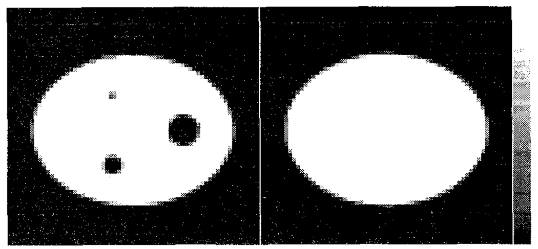
The phantom used in our study (Figure 1) consisted of a water filled 32 × 24 cm elliptical cylinder with infinite axial extent. The cylinder contained cold rods of 1, 3 and 5 cm diameter placed in a uniform background activity of Tc-99m. It was digitized into a 64 × 64 matrix, with 0.625 cm pixels, and only the 3,388 pixels lying within an inscribed circle were considered elements of the object space. Note that the analytical version of the phantom was used for the Monte Carlo simulations so that errors due to pixelization effects were avoided.
Fig. 1.
Images of the cylindrical phantom (left) and attenuation map (right).
B. Projection Data
The SIMIND [20] Monte Carlo program was used to simulate a SPECT acquisition using a gamma camera equipped with a low energy high resolution (LEHR) parallel hole collimator. The energy resolution of the camera was 11% at 140 kev and varied as l/sqrt(energy). The effects of attenuation and ten orders of scatter (including coherent scatter) were included in the simulation, but photon interactions within the collimator were excluded. Since the phantom was uniform along the axial direction, projection data were simulated for only one slice. However, scatter from other slices into the slice of interest was included. In this way, the contribution of scattered photons for the 3D situation was accurately simulated for the case of a source which was uniform in the axial direction.
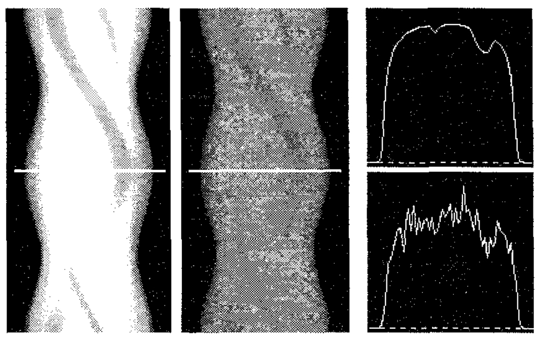
A large number (8.7×10⁷) of photon histories were simulated at each of 128 projection angles spanning 360°, resulting in projection data that were essentially noise-free. We simulated 128 projections at each angle, and these were later collapsed to form 64 bins, each 0.625 cm wide. The projection data were simulated using 1 kev wide energy windows and were later summed to form the energy window combinations described in the next section. After forming the energy windows, Poisson noise was simulated in each corresponding to an acquisition which acquired 3×10⁵ total counts in a 20% wide photopeak energy window. Example sinograms are shown in Figure 2 to help the reader assess the noise-free quality of the simulated data relative to the noise level studied.
Fig. 2.
Sinograms of the essentially noise-free Monte Carlo simulated projection data (left) and noisy projection data (center) at a count level of 3×10⁵ total counts. Horizontal profiles of one angle of the noise-free (top) and noisy (bottom) projection data are shown at the right.
C. Energy Window Combinations
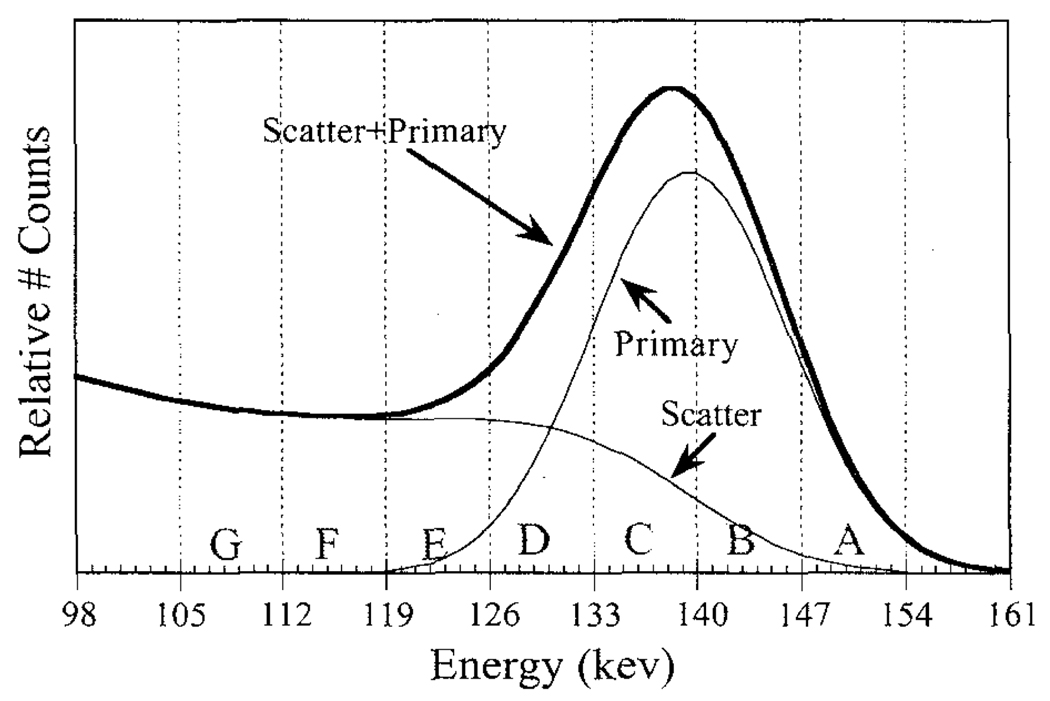
The energy spectrum of the projection data is shown in Figure 3. Seven 7 kev wide energy windows were defined over the range of 105–154 kev and labeled by the letters A–G as shown. These windows were combined to produce the single and multiple window projection data sets described in Table I. For example, the 20% wide photopeak energy window includes photons from 126–154 kev, and is described by the sum of four 7 kev wide windows: ABCD.
Fig. 3.
Histogram of measured energy spectrum and labeling of the 7 kev wide energy windows A–G.
Table I.
Single and multiple energy window projection data sets used in the study.
| Projection data set |
Description |
|---|---|
| non-RBSC Methods: | |
| Perfect Scatter Rejection |
ABCD accepting only primary photons |
| Ideal Scatter Subtraction |
ABCD with noise-free scatter component subtracted |
| RBSC Methods: | |
| 20% Photopeak Window |
ABCD = 126–154 kev window with scatter modeling |
| 49 kev Window | ABCDEFG = 105–154 kev with scatter modeling |
| Contiguous | A, B, C, D, E, F, G = Seven small windows, each with scatter modeling |
| Alpha | AD, B, C, EFG = Four windows, one of which is discontinuous, each with scatter modeling. |
The data sets can grouped into two categories: (i) those including only photons near the emission peak, and (ii) those including lower energy photons as well. The methods studied which use data sets in category (i) include: (1) acquiring scatter and primary photons with modeling of the scatter response function in the transfer matrix used in the reconstruction (reconstruction-based scatter compensation, RBSC); (2) acquiring primary photons only (perfect scatter rejection);and (3) acquiring scatter and primary photons followed by subtracting the mean (noise-free) scatter component (ideal scatter subtraction). In the last two cases the transfer matrix used for the reconstructions modeled only the primary photons since scattered photons were not present.
For the category (ii) data sets only RBSC was studied. In all cases a single transfer matrix that included an appropriate scatter model in each energy window was used. The cases using multiple energy windows (e.g. Contiguous and Alpha) provide more projection data points, hence there are more equations describing the activity distribution, and the transfer matrix F is larger for these data sets. Alpha was chosen in such a way that each of its four windows had roughly the same number of counts.
D. Transfer Matrices
Transfer matrices for each of the windows and combinations discussed above were generated using models for the effects of attenuation, detector response, and scatter (slab-derived scatted estimation method, Frey et a1 [6,7]; Beekman et al [21] have proposed an essentially identical scatter model). Factors were included accounting for the fraction of total counts reaching each window, making each transfer matrix quantitatively accurate. Monte Carlo methods could also have been used to generate the transfer matrices [10,22]; however, using models to generate the transfer matrices is much faster. When models are used, inconsistencies between the simulations and the models will be experienced as errors in the signal power spectrum and bias in the reconstructed images. By comparing the MSPLSV for Monte Carlo generated projection data with the MSPLSV of projection data generated using the modeled transfer matrix, the effects of inaccuracies in the model can be observed. Preliminary investigations in this area have indicated some discrepancies between signal powers for Monte Carlo and model generated projection data at higher singular value indices, indicating there is some breakdown of the models for high frequency information.
E. Singular Value Decompositions
Due to the large size of F (in our case, up to 250 million elements) a computer with very large memory is required to perform the SVD. To reduce memory requirements, we perform the SVD on the product FTF, which is much smaller (~11 million elements). Since FTF is symmetric, its SVD leads to left and right singular vectors which are identical. A simple derivation can be used to show these are also the right singular vectors of F. In addition, the singular values of FTF are the squares of those of F. However, the left singular vectors of F are not calculated explicitly during the SVD of FTF, and must be calculated later as:
| (8) |
All computations were performed on a Cray YMP at the North Carolina Supercomputer Center using Cray single precision (64-bit) floating point. SVDs were performed using the LAPACK [23] routine SGESVD, and required approximately 18 minutes of CPU time for decomposition of a 3,388 × 3,388 matrix. Computation of the matrix UT required about 22 minutes per energy window, and once UT was obtained, the spectra were generated in seconds.
IV. RESULTS
A. Singular Value Spectra
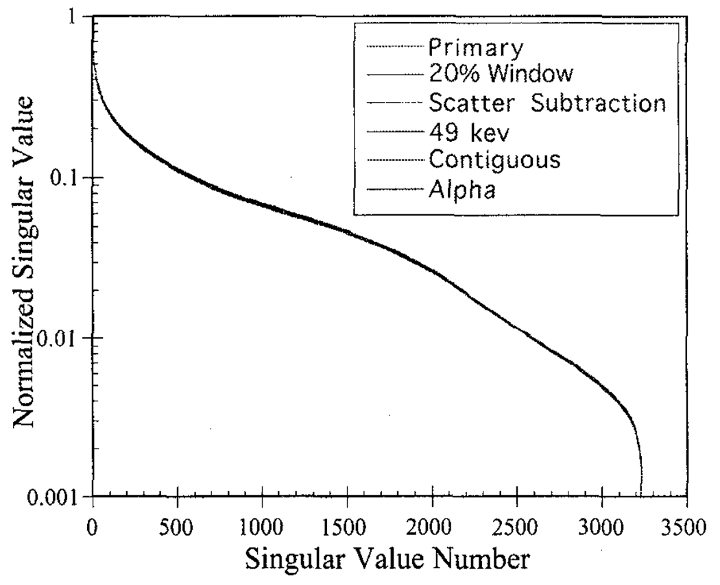
Figure 4 shows the singular value spectra for each case studied. The spectra have been normalized so that the largest singular value is one in each. The contiguous windows case had a nullity (dimension of null space) of 9, and all other cases had a nullity of 8; however, for all cases the singular values beyond index 3,228 were so small that we treated them as numerically singular. We divided the largest singular value by the 3228th one and found this ratio varied by less than 3% for all cases. The similarity of these singular value spectra indicates that, in the absence of noise, including scattered photons, even low energy ones, and using reconstruction-based scatter compensation does not adversely affect the invertibility of the system.
Fig. 4.
Singular value spectra for each of the cases studied, normalized so that the largest singular value is one. The singular value spectra were found to be nearly identical for all cases.
B. Power Spectra
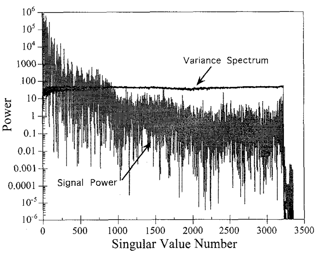
Figure 5 shows the signal power and variance spectra for reconstruction-based scatter compensation using the 20% wide photopeak energy window at a noise level of 3×10⁵ total counts. The “noisy” appearance of the signal power spectrum is due to the ordering of the singular values from largest to smallest and is not related to statistical noise. The figure clearly shows how the signal power tends to be higher than the variance for the larger singular values (smaller singular value number), and then drops below the variance. A typical regularization scheme for a GMI reconstruction would be to truncate or roll-off the singular value spectrum at the crossing point so that image components with higher variance than signal power would be suppressed.
Fig. 5.
Signal power and variance spectra expressed using the primary photon left singular vector basis for the RBSC method using a 20% wide photopeak energy window.
It should be noted that, since the fraction of total counts reaching each energy window has been included in calculation of the transfer matrices, the reconstruction method is quantitatively accurate for each energy window. This means that, assuming the data are consistent with the models used to generate the transfer matrices, the signal power spectra for all projection data sets studied are identical. Thus, the variance spectra for each case can be compared in a relative sense since they are each relative to the same signal power.
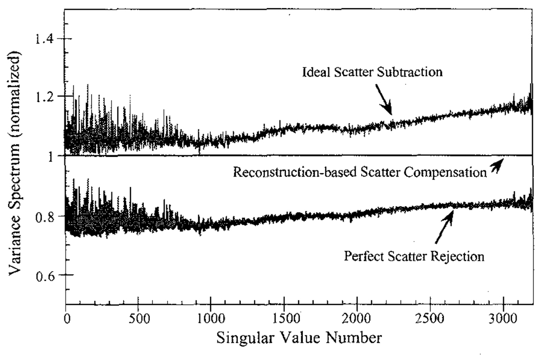
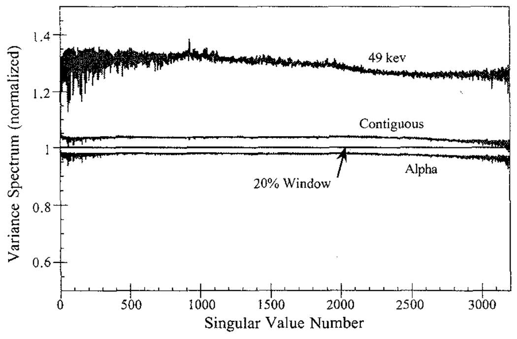
The variance spectra expressed using the primary photon left singular vector basis for each of the cases studied are shown in Figure 6 and Figure 7. The data correspond to a noise level of 3×10⁵ total counts in the 20% window, and the spectra have been normalized so that the variance for the 20% window is one at all singular value indices. Such normalization accentuates the differences relative to the 20% window. The perfect scatter rejection case (primary photons only) was found to have the lowest variance (Figure 6), even though all other cases had more counts because of the inclusion of scatter. This is evidence of the degrading effect of scatter–the wide response function of the scattered photons causes the system to be more sensitive to noise in the projection data. RBSC produced better results than ideal scatter subtraction, due to the fact that the subtraction step results in a higher variance relative to the mean of the subtracted data, These results agree with the results of Frey et al [24] using iterative reconstruction methods.
Fig. 6.
Comparison of variance spectra for the various methods using data in a 20% wide photopeak energy window only. The spectra have been normalized so that the reconstruction-based scatter compensation variance is one at all singular values indices.
Fig. 7.
Comparison of the variance spectra for the various RBSC schemes. Descriptions of the window combinations are given in Table 1. The spectra have been normalized so that the 20% window variance is one at all singular values.
When lower energy photons are included, the 49 kev window was found to have the highest variance, and the remaining two cases were found to have variances similar to the 20% photopeak energy window. The contiguous windows performed slightly worse than the 20% window, and window combination Alpha was somewhat better.
C. Cumulative Normalized Power Differential
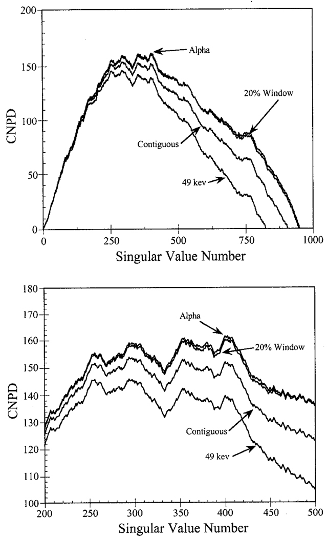
Figure 8 shows the CNPDs for the RBSC methods using low energy photons, where the 20% photopeak window results are included for comparison. The 20% window and window combination Alpha had very similar CNPD spectra and were the highest, followed by the contiguous windows and the 49 kev window. The peak value for combination Alpha, which uses low energy scattered photons, was slightly higher than that for the 20% window. This is evidence of the potential for low energy photons to improve the noise characteristics of the system.
Fig. 8.
CNPD spectra for each case modeling scatter (top), and a blow-up of the peak region of the curves (bottom). The higher the CNPD, the lower the variance relative to the signal power. Window combination Alpha resulted in a slightly higher CNPD than for the 20% window, and the other windows resulted in markedly lower CNPD values.
Though the CNPD peak for Alpha is slightly higher than that for the 20% window, the improvement is less than one would expect from looking at the variance spectra shown in Figure 7. The reason is that there are discrepancies between the Monte Carlo simulations and the scatter model for the low energy windows. This leads to small errors in the signal power for Alpha at higher singular value numbers, and the CNPD is reduced. These errors could be eliminated by using improved models, which would result in a CNPD for Alpha which is higher than that for the 20% window, as predicted by the variance spectra results.
D. Reconstructed Images
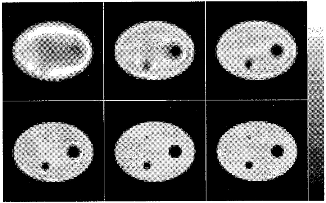
We now present a series of GMI reconstructed images and corresponding variance images to demonstrate that the power spectra results accurately predict reconstructed image noise levels. Figure 9 shows reconstructed images at six degrees of regularization for the perfect scatter rejection case using noise-free projection data. The images indicate how image quality is affected by the degree of regularization. The remaining results presented in this section are for images regularized by truncating the singular value spectrum beyond index number 2000 (lower left image of Figure 9).
Fig. 9.
Noise-free reconstructed images for the perfect scatter rejection case for six degrees of regularization. Top row, left to right: 500, 1000, 1500 singular values included; Bottom row, left to right: 2000, 2500, 3000 singular values included.
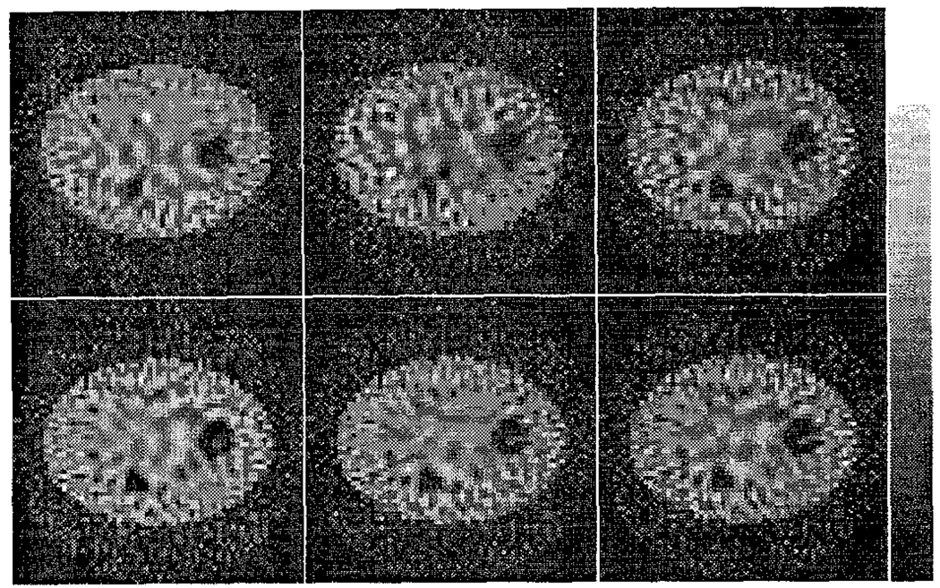
Images reconstructed from noisy projection data for each of the cases studied are shown in Figure 10. Poisson noise was simulated for a count level of 3×10⁵ total counts in the 20% wide photopeak energy window. Differences in the noise magnitude and texture can be seen in these images. For example, the 3 and 5 cm diameter rods are clearly more distinct in the RBSC images than in the ideal scatter subtraction image, and marginally more distinct than in the perfect scatter rejection image.
Fig. 10.
GMI Reconstructed images (2000 singular values included) of the noisy projection data. Top row: Perfect scatter rejection (left), ideal scatter subtraction (center), and RBSC with a 20% wide photopeak window (right); Bottom row: RBSC using the 49 kev window (left), Contiguous windows (center), and windows Alpha (right).
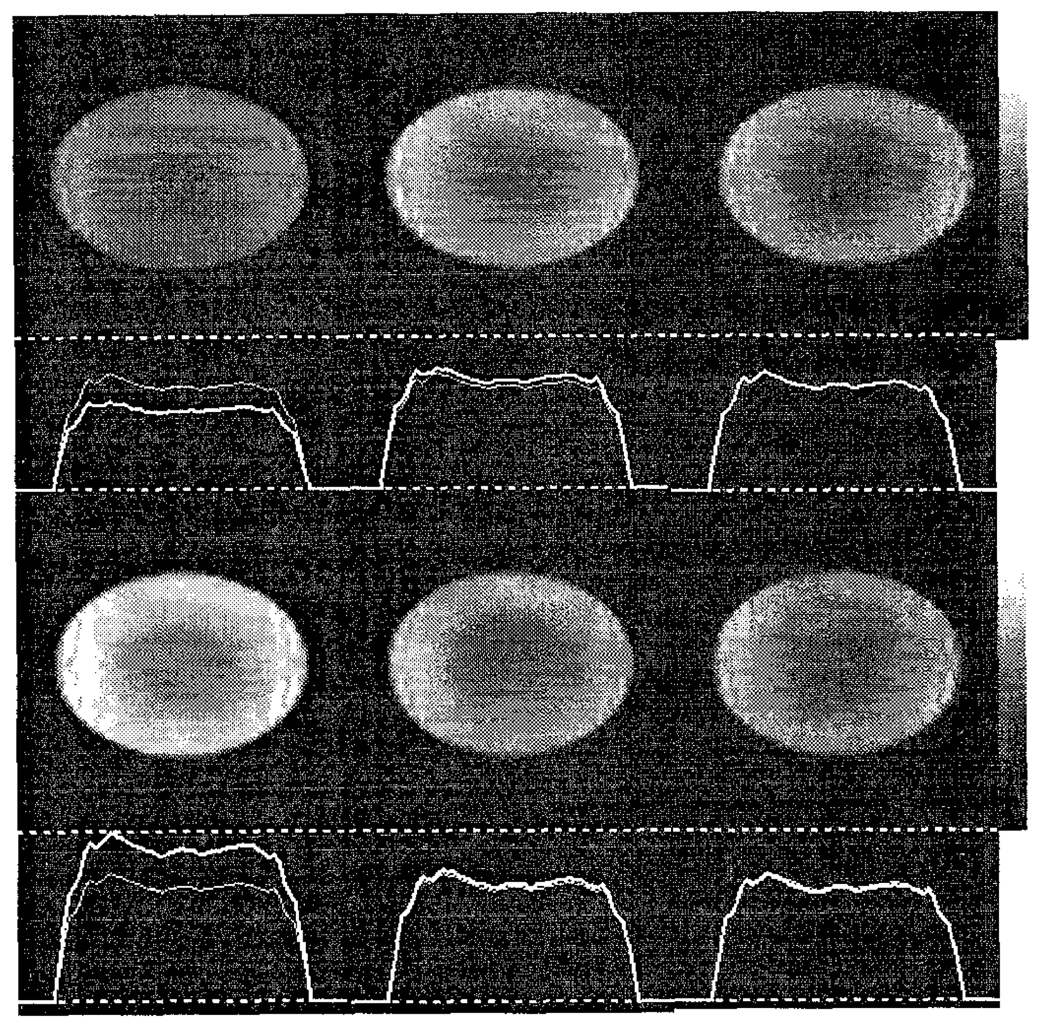
To quantify the noise magnitude of the GMI reconstructed images, corresponding variance images were calculated analytically (see section II.C.). In all cases, the variance images were found to correlate with the variance power spectra and CNPD results presented earlier in this paper. Variance images corresponding to the reconstructed images shown in Figure 10 are shown in Figure 11 (2000 singular values included). Pixels lying outside of the phantom contour have been zeroed to make the variance images easier to understand. Horizontal profiles across the full height of each variance image are also shown in Figure 11, and the profile for the 20% window case has been overlain on each to make relative comparison of each case easier. The figure also demonstrates that the reconstructed image noise is clearly non-stationary. By comparing the relative heights of the profiles in Figure 11, the variance image results can be seen to agree with the power spectra results presented earlier. Again, the choice of energy windows was found to critically affect the noise levels of the reconstructed images.
Fig. 11.
Variance images accompanied by horizontal profiles corresponding to the images shown in Figure 10. The profiles are all normalized to the peak height of the 49 kev window profile (bottom left), and the 20% window profile (top right) has been overdrawn on each profile (thinner line) to allow easier comparison.
The reader should note that the variance doesn’t give all the information about the noise in the image: the covariance should also be calculated [25,26]. The covariance gives information about noise texture; that is, about the size and shape of the noise “blobs” in the image. It has been conjectured that only noise correlation is important to human observers performing a lesion discrimination task [26]. For example, the 3 and 5 cm rods in the phantom are easier to distinguish in Figure 10 for the RBSC methods than for the perfect scatter rejection case, even though the perfect scatter rejection case had the lowest variance of all cases studied. This might be due to differences in noise correlations in the images; however, we have not calculated the covariance in this paper.
V. Discussion
The results shown in the preceding sections are for the cold rod phantom shown in Figure 1. Since we did not include statistical weights in the system matrix (i.e., we used the unweighted least-squares criterion), the SVDs are valid for any source distribution or count level in the same attenuator. We took advantage of this by repeating the analysis for five different contrast levels (ranging from cold rods in a hot background to hot rods in a cold background) and four different count levels. In all cases the results agreed with those for the cold rod phantom shown earlier.
The disadvantage of using the least-squares criterion is that, while the results are similar when all projections have roughly the same number of counts (as is the case when the phantom background is high and only one window is used), statistical weighting may dramatically affect the results when the projections span a wide range of counts. One example is the contiguous windows case. Though the lower energy windows have fewer counts than the windows near the 140 kev peak, the least-squares criterion weights all the windows the same. Thus, low count data is inappropriately weighted as heavily as high count data, and a noisier image results. It is likely the contiguous windows case would have a lower variance than combination Alpha (and, hence, the 20% window) if statistical weights were included. For this reason, the results shown in this paper must be interpreted carefully.
When including low energy photons, the choice of energy window scheme was found to critically affect the noise levels of the system. In particular, multiple energy window schemes were found to result in a lower variance than using a single wide energy window. This result is intuitively appealing because the multiple energy windows provide more information about the activity distribution. The potential for low energy photons to be used to improve the noise characteristics of the system is also supported, as evidenced by the improved noise characteristics for window combination Alpha. However, it appears that statistical weights must be included, as suggested by the poor showing for the contiguous windows, in order to optimize the energy window scheme and to determine the degree of noise reduction. This will be the subject of future research.
VI. Summary and Conclusions
We have used singular value decomposition as a tool for investigating the noise properties of SPECT when modeling scatter in windows spanning a wide energy range. The approach has the advantage of providing information about invertibility and noise propagation which is independent of the choice of iterative reconstruction algorithm and degree of regularization. We have calculated and compared signal power and variance spectra expressed using the primary photon left singular vector basis for several energy window combinations, and computed a metric, termed the cumulative normalized power differential (CNPD), which provides a measure of the balance between signal power and variance as a function of the degree of regularization. We have also calculated variance images for one degree of regularization. For all cases, the power spectra results were found to correlate with the variance of the reconstructed images. The covariance of the images was not studied.
The RBSC results were compared with those from the cases of perfect scatter rejection and ideal scatter subtraction. Perfect scatter rejection resulted in the lowest variance of all cases studied, even though the other cases had more counts because of the inclusion of scattered photons. This is evidence of the degrading nature of scatter–the scattered photon counts in the 20% window have the effect of increasing reconstructed image variance. RBSC performed better than ideal scatter subtraction as expected, because the subtraction step results in a higher variance relative to the mean of the subtracted data.
When low energy scattered photons were included in the projection data and modeled in the reconstructions, the performance was found to be critically dependent upon the choice of energy windows, even when they span the same energy range. Improvements were found using multiple energy windows over using a single wide energy window, and there is evidence that the inclusion of low energy photons may improve the noise characteristics of SPECT. However, statistical weights should be included in the system matrix before the energy window scheme can be optimized and the degree of noise reduction can be determined.
Acknowledgments
This work was supported by a grant # R29-CA63465 from the National Cancer Institute and by an academic research grant from the North Carolina Supercomputer Center. Its contents are solely the responsibility of the authors and do not necessarily represent the official views of the National Cancer Institute or the NCSC.
REFERENCES
- 1.Jaszczak RJ, et al. Improved SPECT quantitation using compensation for scattered photons. J. Nucl. Med. 1984;vol. 25(no 8):893–900. [PubMed] [Google Scholar]
- 2.Axelsson B, Msaki P, Israelsson A. Subtraction of Compton-scattered photons in single-photon emission computerized tomography. J. Nucl. Med. 1984;vol. 25(no 4):290–294. [PubMed] [Google Scholar]
- 3.Ichihara T, Ogawa K, Motomura N, Kubo A, Hashimoto S. Compton scatter compensation using the triple-energy window method for single- and dual-isotope SPECT. J. Nucl. Med. 1993;vol. 34(no 12):2216–2221. [PubMed] [Google Scholar]
- 4.King MA, Hademenos GJ, Glick SJ. A dual-photopeak window method for scatter correction. J. Nucl. Med. 1992;vol. 33(no 4):605–612. [PubMed] [Google Scholar]
- 5.Koral KF, Wang X, Rogers WL, Clinthorne NH, Wang X. SPECT Compton-scattering correction by analysis of energy spectra. J. Nucl. Med. 1988;vol. 29(no 2):195–202. [PubMed] [Google Scholar]
- 6.Frey EC, Tsui BMW. A practical method for incorporating scatter in a projector-backprojector for accurate scatter compensation in SPECT. IEEE. Trans. Nucl. Sci. 1993;vol. NS-40(no 4):1107–1116. [Google Scholar]
- 7.Frey EC, Ju Z-W, Tsui BMW. A fast projector-backprojector pair modeling the asymmetric, spatially varying scatter response function for scatter compensation in SPECT imaging. IEEE. Trans. Nucl. Sci. 1993;vol. NS-40(no 4):1192–1197. [Google Scholar]
- 8.Kadrmas DJ, Frey EC, Tsui BMW. Improved signal-to-noise ratio in SPECT images by simultaneous reconstruction from multiple overlapping energy windows. J. Nucl. Med. 1995;vol. 36(no 5):29. [Google Scholar]
- 9.Frey EC, Tsui BMW. Use of the information content of scattered photons in SPECT by simultaneous reconstruction from multiple energy windows. J. Nucl. Med. 1994;vol. 35(no 5):17. [Google Scholar]
- 10.Golub GH, Loan CFV. Matrix Computations. Baltimore: John Hopkins University Press; 1989. [Google Scholar]
- 11.Press WH, et al. Numerical Recipes in C. Cambridge: Cambridge University Press; 1988. [Google Scholar]
- 12.Smith MF, Floyd CE, Jr, Jaszczak RJ, Coleman RE. Reconstruction of SPECT images using generalized matrix inverses. IEEE Trans. Med. Imag. 1992;vol. MI-11(no 2):165–175. doi: 10.1109/42.141640. [DOI] [PubMed] [Google Scholar]
- 13.Gullberg GT, Huesman RH, Zeng GL, Foresti SA. Efficient estimation of dynamic cardiac SPECT kinetic parameters using weighted least square estimates of dynamic reconstructions. Conference Proceedings of the 1995 IEEE Nuclear Science Symposium and Medical Imaging Conference; in press. [Google Scholar]
- 14.Smith MF. Generalized matrix inverse reconstruction for SPECT using a weighted singular value spectrum. Conference Proceedings of the 1995 IEEE Nuclear Science Symposium and Medical Imaging Conference; in press. [Google Scholar]
- 15.Zeng GL, Gullberg GT. Does truncation always result in an under-determined problem? - An SVD study. Conference Proceedings of the I995 IEEE Nuclear Science Symposium and Medical Imaging Conference; in press. [Google Scholar]
- 16.Gregoriou GK, Tsui BMW, Frey EC, Lalush DS. Artifacts and sampling requirements in transmission CT reconstruction with truncated projection data. Conference Proceedings of the 1995 IEEE Nuclear Science Symposium and Medical Imaging Conference; in press. [Google Scholar]
- 17.Papoulis A. Probability, Random Variables, and Stochastic Processes. McGraw-Hill Book Company; 1965. [Google Scholar]
- 18.Kijewski MF, Judy PF. The noise spectrum of CT images. Phys. Med. Bio. 1987;vol. 32(no 5):565–575. doi: 10.1088/0031-9155/32/5/003. [DOI] [PubMed] [Google Scholar]
- 19.Riederer SJ, Pelc NJ, Chelser DA. The noise power spectrum in computed tomography. Phys. Med. Bio. 1978;vol. 23(no 3):446–454. doi: 10.1088/0031-9155/23/3/008. [DOI] [PubMed] [Google Scholar]
- 20.Ljungberg M, Strand S-E. A Monte Carlo program for the simulation of scintillation camera characteristics. Comp. Meth. Prog. Biomed. 1989;vol. 29:257–272. doi: 10.1016/0169-2607(89)90111-9. [DOI] [PubMed] [Google Scholar]
- 21.Beekman F, et al. Object shape dependent PSF model for SPECT imaging. IEEE. Trans. Nucl. Sci. 1993;vol. NS-40(no 1):31–39. [Google Scholar]
- 22.Floyd CE, Jaszczak RJ, Coleman RE. Inverse Monte Carlo: a unified reconstruction algorithm. IEEE. Trans. Nucl. Sci. 1985;vol. NS-32(no 1):779–785. [PubMed] [Google Scholar]
- 23.Anderson E, Bai Z, Bischof C, Demmel JW, Dongarra JJ, Du Croz J, Greenbaum A, Hammarling S, McKenney A, Sorenson D. LAPACK: A portable linear algebra library, for high-performance computers. Knoxville: Computer Science Dept. Technical Report CS-90- 105, University of Tennesse; 1990
- 24.Frey EC, Tsui BMW, King MA, Ljungberg M. A quantitative comparison of extended dual photon window and iterative reconstruction based scatter compensation. J. Nucl. Med. 1993;vol. 34(no 5):72P. [Google Scholar]
- 25.Wilson DW. dissertation. Chapel Hill, N.C.: The University of North Carolina at Chapel Hill; 1994. Noise and resolution properties of FB and ML-EM reconstructed images. [Google Scholar]
- 26.Wilson DW, Tsui BMW, Terry JA. Non-stationary noise characterization for SPECT images produced using several reconstruction filters and attenuation compensation techniques. Ann. Biom. Eng. 1991;vol. 19(no 5):610. [Google Scholar]


