Exploring classification strategies with the CoEPrA 2006 contest

Abstract

Motivation: In silico methods to classify compounds as potential drugs that bind to a specific target become increasingly important for drug design. To build classification devices training sets of drugs with known activities are needed. For many such classification problems, not only qualitative but also quantitative information of a specific property (e.g. binding affinity) is available. The latter can be used to build a regression scheme to predict this property for new compounds. Predicting a compound property explicitly is generally more difficult than classifying that the property lies below or above a given threshold value. Hence, an indirect classification that is based on regression may lead to poorer results than a direct classification scheme. In fact, initially researchers are only interested to classify compounds as potential drugs. The activities of these compounds are subsequently measured in wet lab.

Results: We propose a novel approach that uses available quantitative information directly for classification rather than first using a regression scheme. It uses a new type of loss function called weighted biased regression. Application of this method to four widely studied datasets of the CoEPrA contest (Comparative Evaluation of Prediction Algorithms, http://coepra.org) shows that it can outperform simple classification methods that do not make use of this additional quantitative information.

Availability: A stand alone application is available at the webpage http://agknapp.chemie.fu-berlin.de/agknapp/index.php?menu=software&page=PeptideClassifier that can be used to build a model for a peptide training set to be submitted.

Contact: odemir@chemie.fu-berlin.de

Supplementary Information: Supplementary data are available at Bioinformatics online.

1 INTRODUCTION

Molecular classification problems are common in many fields of chemistry, biochemistry, pharmacy, medicinal diagnostics and other applications in modern life sciences. In an empirical regression or classification problem, one considers objects that possess a specific common relationship characterized by object-specific target values. For drug molecules, these target values may relate to a property that characterizes binding. In a regression problem, these target values vary continuously in an interval. These can for instance be binding affinities of drugs that bind to the same receptor. For a classification problem, the objects are labeled according to the group they belong to using discrete target values. To solve a classification or regression problem, we need to correlate the individual objects with their respective target values. Target values for a two-class classification problem are for instance t = +1/−1 that can be used to characterize objects of the positive/negative class. To construct an empirical device (regressor or classifier) to predict unknown target values one needs a training set of related objects with known target values. Such molecular regression and classification problems are addressed in the Comparative Evaluation of Prediction Algorithms (CoEPrA) 2006 competition (http://www.coepra.org/). The CoEPrA competition can be seen in analogy to CASP (Critical Assessment of Techniques for Protein Structure Prediction) (Dunbrack et al., 1997) that focuses on protein structure prediction, while CoEPrA deals with regression and classification problems of biological active molecules.

On an average, 15 research groups participated in the four CoEPrA 2006 classification contests. To solve the classification tasks different approaches were used by the participating groups ranging from applications of support vector machine (SVM) (Boser et al., 1992; Vapnik, 1995), artificial neural networks (Haykin, 1998), naive Bayesian decision theory (Duda et al., 2005; Minsky, 1961), least-square optimization (Fisher, 1936), decision trees (Breiman et al., 1984), random forest methods (Breiman, 2001) and new classification methods such as kScore (Oloff and Muegge, 2007).

CoEPrA considers exclusively oligopeptides from which the sequences and alternatively physico-chemical descriptors comprising many different features were provided at the CoEPrA webpage. In a way a classifier (regressor), ‘observes’ the objects (molecules) through eyes that are defined by the features used as descriptor. Other sets of features considering global physico-chemical and sterical properties of the whole peptide (such as volume, molecular weight, or solvent accessible surface area) or evolutionary residue similarities such as Blosum Matrices (Henikoff and Henikoff, 1992) can be used alternatively.

Since the number of peptides for each classification and regression task of CoEPrA is very small, the number of descriptors has to be small as well to avoid over parameterization. This was solved by the participants in different ways. Some used small feature sets like the peptide sequence-based features, others massively reduced the number of physico-chemical features by applying principal component analysis (Jackson, 1991; Pearson, 1901), genetic algorithms (Vafaie and Jong, 1992), ant colony optimization (Al-Ani, 2005) or simple filters (Guyon and Elisseeff, 2003). This wide range of methods applied by different groups makes the CoEPrA contest an ideal test ground to explore different training and prediction schemes.

When predicting a certain property of a molecule, researchers are often just interested whether the value of this property is below or above a certain threshold. Thus, one can classify candidate molecules from a large set of molecules. For the most interesting molecules, the property values are subsequently measured in wet lab. However, when building predictors the exact property (or target) values are often available. This information is routinely used when building a regressor, which tries to predict the property values for new molecules. But, predicting property values is more demanding than to predict just the classes to which the molecules belong to. Hence, predicting a property value by regression with subsequent classification is expected to introduce larger uncertainties than solving the classification problem directly. But, the additional information of the specific property values could be of use to solve the classification problem more reliably. The classification methods used in this study consider such quantitative information of the target value directly that is normally only used for regression. Thus, improving classification results considerably.

2 METHODS

2.1 CoEPrA data sets of oligo-peptides

CoEPrA 2006 offered four classification and four regression tasks. Each classification task consists of two independent data sets of oligo-peptides (octo-peptides for task 2 and nona-peptides for the other three tasks) one for training with known binding affinity and one for prediction with unknown binding characteristics. The latter were revealed after the contest. After the contest, it became evident that all oligo-peptides used for classification and regression tasks of CoEPrA 2006 are ligand peptides of the major histocompatibility complex (MHC) (Krogsgaard and Davis, 2005; Kuhns et al., 1999), an important player of immune response in mammals. The classification tasks of the oligo-peptides presented by CoEPrA are based on experimentally measured binding constants or the related pIC50 values. For the CoEPrA regression tasks, the pIC50 values are the target values. The classification tasks 1, 2, 3 consist of symmetric data sets, i.e. the number of binding and non-binding ligands are for training and prediction sets essentially equal, while the dataset of task 4 is asymmetric possessing more non-binding than binding ligands. Table 1 contains a summary of the four CoEPrA data sets for classification.

Table 1.

The four CoEPrA data sets for classification

Tasks	Traininga		Predictionb		Lc
# (literature with pIC50 values)	Pos	Neg	Pos	Neg
1d(Doytchinova et al., 2005)	45	44	44	44	9
2d(Hattotuwagama et al., 2004)	37	39	38	38	8
3d(Doytchinova and Flower, 2002)	67	66	67	66	9
4 (Source unknown)	19	92	19	92	9

^aNumber of ligands in training set with known classification of binding (pos) and non-binding (neg) oligo-peptides.

^bNumber of ligands in prediction set; classification of binding (pos) and non-binding (neg) oligo-peptides was unraveled only after termination of contest.

^cLengths of oligo-peptides for the four classification tasks.

^dpIC50 value available.

For three CoEPrA classification tasks (tasks 1, 2, 3), the joint sets of binding and non-binding oligo-peptides are for prediction and training the same as for the corresponding CoEPrA regression tasks. In contrast to regression, classification requires to separate the sets into two groups. In order to do so, the organizers of CoEPrA 2006 used pIC50 threshold values T_pIC50 to assign the oligo-peptides to the binding (t=+1) or non-binding (t=−1) class (Doytchinova and Flower, 2001, 2002).

Although these threshold values were not published, it is possible to extract them approximately from the pIC50 values given for the CoEPrA regression tasks 1, 2, 3. These threshold values are 5.3900, 7.7810 and 7.0725 pIC50 for the CoEPrA classification task 1, 2, 3, respectively. In Figure 1, the pIC50 values are displayed for each set of oligo-peptides sorted by rising values. Thus, the non-binding peptides are displayed in the lower left while the binding peptides appear in the upper right of this diagram. Histograms of the binding affinities are given in the Supplementary Material (Supplementary Fig. S1). For all three sets, the distributions of pIC50 values are very similar for the training and the prediction set, which is a prerequisite to perform predictions successfully. However, there are differences in the distributions of the three tasks. For task 1, the pIC50 values vary from 3 to more than 8, while these intervals are smaller for task 2 and 3, where the pIC50 values vary only from 5 to 8 and 5 to 9, respectively. Near to the threshold (solid horizontal line in Fig. 1) discriminating between binding and non-binding peptides the slope of the pIC50 values is much smaller for task 2 than for the other two CoEPrA tasks. Furthermore, task 1 and 3 exhibit for training and prediction approximately a point symmetry with respect to the distributions of binding and non-binding peptides, which is absent for task 2. This all indicates that prediction might be easier for the first task than for the second and third task, which roughly correlates with the success of the participants in the CoEPrA contest.

Fig. 1.

Binding affinities in terms of pIC50 values for the first three CoEPrA tasks sorted with increasing pIC50 value. The solid horizontal lines mark the threshold used to group the peptides into binders and non-binders. (A) Training sets that were used to build the models. (B) Prediction sets used to estimate performance. Histograms of the binding affinities are given in the supporting material (Supplementary Fig. S1).

2.2 Features used for the CoEPrA datasets

Training a prediction device for classification requires to correlate features describing the data points (objects) of the training set with their corresponding class-specific target values (+1, −1). Since CoEPrA 2006 provides the sequences of the oligo-peptides one can use these directly or generate own features, which was done by several groups participating in the contest. Alternatively one can use the physico-chemical features given by CoEPrA to describe the oligo-peptides. Those physico-chemical features are amino acid specific features taken from the literature (Kawashima and Kanehisa, 2000; Kawashima et al., 1999). The physico-chemical features of CoEPrA describe each amino acid by 643 features whose values are given by real numbers resulting in a total number of 5787 or 5144 features for nona- or octo-peptides, respectively. Each of these features describes a physico-chemical property of a single amino acid.

The simplest set of sequence based features is to assume that all amino acids are equidistant. In such a case, we can represent the 20 native amino acids by 20 component vectors for amino acid type Q. All components of this vector are zero except for the position encoding the considered amino acid type where the value of the component is unity (sparse binary descriptor). In this case, we use the simple metric that all amino acid pairs have the same degree of similarity. This was the amino acid representation that we used in the CoEPrA competition. Thus, the total number of features is 180 for nona-peptides and 160 for octo-peptides.

Another representation using also a 20 component feature vector per amino acid is to characterize the amino acids by the integer values of a Blosum matrix (Block substitution matrix) (Henikoff and Henikoff, 1992). Blosum matrices are generated from multiple sequence alignments of protein sequences that share a certain amount of sequence identity. The Blosum matrices contain the information on how likely it is that a certain amino acid can mutate into another. Positive values imply a high negative values a low probability for such mutations. In other words, positive entries refer to other amino acids that possess common biochemical properties and thus can be exchanged more easily without alternating the behavior of a protein, whereas negative values refer other amino acids that are rather dissimilar. There are different Blosum matrices labeled by numbers that differ by the protein similarity that was used to generate the multiple sequence alignments. BlosumX matrices with a small X value describe amino acid similarities of evolutionary more distant proteins, whereas BlosumX matrices with a large X value describe amino acid similarities of highly related proteins. In our studies, different Blosum matrices where used: Blosum40, Blosum62 and Blosum90. The Blosum62 matrix yielded the best overall performance in our applications and is also the default for many sequence alignment applications (Altschul et al., 1997). Analog to the sparse descriptor the oligo-peptides are described by feature vectors of lengths 180 or 160 for nona- or octo-peptides, respectively.

Since the encoding techniques with three different types of features have specific merits and disadvantages we also build models for all four possible combinations of them (sparse/Blosum; sparse/physico-chemical; Blosum/physico-chemical; sparse/Blosum/physico-chemical). Especially, when using physico-chemical features or combinations involving them the features represent many different properties and therefore are given in different units. Thus, it is important to normalize feature vectors before training a classifier. However, before that all features whose standard deviation for the training set vanishes are removed, since they do not contain information. The remaining features are shifted and scaled such that each feature has a mean of zero and a standard deviation of unity relative to the training set. These transformations are then also applied to the prediction set.

2.3 Linear discriminant function

Each oligo-peptide i of the training and the prediction set can be characterized by features combined in a vector in a d dimensional feature space. The decision whether the oligo-peptide is binding (target value t = +1) or non-binding (target value t = −1) can be made by a linear scoring function defined by

(1)

where is the model parameter vector of the scoring function and b ∫ P the threshold or bias. Positive values of the scoring function correspond to one class (t = +1) negative to the second class (t = −1). Setting the linear scoring function to zero describes a hyperplane in the d-dimensional feature space P^d defining two half-spaces that correspond to the two classes. The orientation of the hyperplane is defined using the model parameter vector as normal vector of the plane, while its distance from the origin is defined by the threshold value b as (b/. A data point with vector is classified as positive, if and as negative, if .

Note that for this type of scoring functions the number of model parameters is d+1, where d is the number of features. The d+1 model parameters are optimized during the so-called training phase where data with known classification are used to determine the hyperplane that is able to separate the binding form the non-binding training samples. Predictions of new samples can be performed by evaluating the sign of the scoring function.

2.4 Mean-squared error loss function

To determine an optimal parameter vector we use an objective function, which is minimized to yield a solution of the hyperplane. Given a set of n training sequences with their feature vectors we define the objective function

(2)

where f(s_i), s_i ∫ P is the so-called loss function. Different loss functions lead to hyperplanes with different properties. A common loss function for classification is the mean-squared error (MSE) loss function for classification (Fisher, 1936)

(3)

with target values t_i=+1, if corresponds to a positive data point and t_i=−1, if corresponds to a negative data point. Minimizing the objective function , b) leads to a solution where the scoring function assumes approximately the value +1 for all positive data points and −1 for all negative data points in the training set. An analog approach was used before using the sparse descriptor to classify MHC nona-peptides (Riedesel et al., 2004).

As described earlier, the first three CoEPrA classification tasks have corresponding regression data sets. Hence, besides the information that a peptide is positive or not each peptide of task 1 to 3 is characterized by its pIC50 binding affinity. To consider the latter information, we use the following loss function

(4)

where pIC50_i denotes the binding affinity of peptide i. Thus, minimizing the objective function leads to a hyperplane where the distances of the data points to the hyperplane are proportional to their measured pIC50 values. This technique is known as regression and the resulting model predicts the binding affinities instead of the target value of the corresponding class. However, a regression result can also be used for classification. For that purpose, all peptides with a predicted pIC50 value larger than a given threshold T are considered as positives, whereas all peptides with a predicted pIC50 value smaller or equal to T are considered as negatives or vice versa depending on the biological problem and the definition of the classes.

2.5 Weighted biased regression loss function

For the regression problem, pIC50 values need to be predicted, which is more difficult than to predict the classes to which the peptides belong to. Hence, the outcome of a prediction based on regression is expected to introduce larger uncertainties than solving the classification problem directly. Nevertheless, the binding affinity contains additional information, which could be of use to solve the classification problem. Therefore, this information should be included in model building. In order to do so, we defined a specific loss function called weighted biased regression (WBR) loss function. This loss function incorporates the binding affinity information to build a classifier rather than a regression scheme

(5)

where y_i ∫[+1, −1] denotes the class label of data point i with y_i=+1, if is a positive data point and y_i=−1, if is a negative data point. Note that we are interested in a parameter vector such that all positive data points are above the classification threshold ( and all negative data points are below the classification threshold (s=). However, we are not interested to match the pIC50 value of a peptide with the scoring function g exactly. Hence, positive data points with a predicted pIC50 value equal or larger than their measured pIC50 value are not penalized by setting f^WBR_class(s_i)=0, since these data points are classified correctly anyway. If the predicted pIC50 value is smaller than its measured pIC50 value a penalization similar to the MSE regression is applied using f^WBR_class(s_i)=μ_i(s_i−PIC50_i)². Here, μ_i>0 is an additional parameter that can be used to weight each data point individually. All negative data points are treated in an analogue fashion. If the predicted pIC50 value is smaller or equal to its measured pIC50 no penalization is applied, whereas for a predicted pIC50 value larger than its measured pIC50 value a quadratic penalization term according to Equation (5) is used.

Many classification techniques concentrate on those data points that are nearest to the decision boundary, since these data points are most critical and informative. In a SVM classification scheme, the separating hyperplane is determined only by those data points that are nearest to the decision boundary. These data points are the so called support vectors (Burges, 1998). In boosting, training is performed over several weak classifiers reweighting the training set for each classifier such that misclassified data points are weighted higher (Guo and Viktor, 2004). The WBR loss function is also capable of reweighting the training points. To emphasize those data points that are closer to the decision threshold than those that are more distant to it we use the weights μ_i=1/[(s_i−PIC50_i)²+γ²], where γ=0.1 is used to prevent singularities.

2.6 Regularization of the objective function

Empirical devices to predict target values employ classification or regression schemes where model parameters are optimized by using a training set of data points with known target values. This method can suffer from overtraining, i.e. the model parameters are particularly adjusted to recall the target values of the training set, but fail to predict target values of data points, which do not belong to the training set. This so-called learning by heart phenomenon occurs especially when the number data points for training is comparable or even smaller than the number of model parameters. To control this effect, the objective function is usually extended by a so called regularization term of positive weight (0 < λ < 1)

(6)

where λ assumes a predefined value that is not optimized simultaneously with the model parameters and b. Minimizing this enhanced objective function requires to balance the two terms. The regularization term adopts its minimum value, if all components of the parameter vector vanish. Normally, this is in conflict with the first term, which requires specific non-vanishing model parameters. The trade-off is that the model parameters governing the less important features are set to small or even vanishing values, while model parameters referring to features that exhibit strong correlations with the target values are kept. According to the structure of the scoring function, Equation (1), features whose corresponding model parameters vanish are ignored, thus, reducing the complexity of the model. Increasing the strength of the regularization term with a larger λ value leads to a simplified model description with a smaller effective number of model parameters. As a consequence, the recall performance decreases, while simultaneously the prediction performance can increase, which avoids learning by heart. The latter is in particular the case, if the original model contained irrelevant or conflicting features. However, if the regularization term becomes too large by increasing the λ parameter further on not only recall but also prediction performance will decrease, since now also important features may be suppressed.

The art is to optimize the regularization parameter λ by increasing its value just before the point where the prediction performance diminishes. But even very small λ parameters (say λ = 10⁻¹⁰) are useful, since they suppress spurious singularities, which may arise from the usage of linear dependent features. The optimal λ value has to be chosen carefully. This can be done automatically by evaluating the prediction performance observing the error in n-fold cross-validation. For that purpose, we define a candidate set of λ values [10⁻⁴, 10⁻³, 10⁻², 0.1, 0.2, 0.3 … 0.9, 0.93], which contains a range of λ values to be tested. For each value of this set, the training set is randomly divided into n parts. One part is retained as a validation set while the other n − 1 parts are used to train the classifier. This process is repeated n times such that each part is used exactly once as validation set. The average over these n validation errors is the estimated performance. The λ value that reveals the smallest validation error is then used to train the classifier on the whole dataset.

2.7 Data balancing

In the case that the number of positive and negative data points is highly unbalanced or if one of the two classes should get a higher weight, since one would like to avoid false positives for that class, it could be reasonable to split up the positive and negative data points leading to the objective function

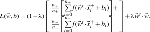(7)

In expression (7), the first sum runs over all positive while the second sum runs over all negative data points in the training set, where n₊ and n₋ (n₊+n₋=n) denote the number of positive and negative data points, while w₊ and w₋ (w₊+w₋=1) are the weights for the positive and negative data points, respectively. Here, we use only w₊=w₋=0.5.

2.8 Training

Since in all cases considered here, the objective function is quadratic in the parameters and b, the minimum of the objective function can be obtained analytically solving a corresponding linear equation (Riedesel et al., 2004) with the Cholesky decomposition (Bau and Trefethen, 1997). Note that the WBR loss function is a recursively defined function, since the model parameters , b depend on the loss function and vice versa. Minimizing the objective function in this case is performed iteratively starting with zero values for all parameters , b₀, using the resulting definition of the WBR loss function, Equation (5), to determine the minimum of the objective function, Equation (7) that yields a new set of parameters , b₁ as solution of the linear equation system. With these parameters a new definition of the WBR loss function is obtained and the objective function can be minimized again. This procedure is repeated until convergence is reached.

2.9 Quality measurement

The quality of the predictions listed in the results section are characterized by the Matthews correlation coefficient (MCC) (Baldi et al., 2000), which combines the prediction results for binding and nonbinding data points in a single numerical value. The MCC ranges from −1 to +1. An unsuccessful, purely random prediction yields MCC=0, while MCC=+1 is a perfect prediction.

3 RESULTS

3.1 General considerations

For each individual classification approach, we use only data from the training set. However, we subsequently compare prediction performances for the different approaches while knowing the outcome. Therefore, we can select the most successful approach. In doing so, we use implicitly information on the prediction dataset such that it is no longer an unbiased prediction as it was for the participants of the CoEPrA contest, which did not even know the predictions of the competitors before the contest was terminated. Therefore, in this study we do not claim that our best approach is truly superior to the best approaches in the CoEPrA contest, if applied to a new problem. Conversely, since we are comparing our approaches with a large number of alternative approaches submitted by the participants in the CoEPrA prediction contest, being close to the best results is quite a challenge.

To relate the results of the present study with the CoEPrA contest results all tables that display the prediction results of this study contain also the results of the best and second best CoEPrA competitor. No competitor obtained the best prediction results in all four CoEPrA prediction contests, although one group came close to it.

3.2 Classification with the MSE classifier

Table 2 shows the prediction results for the simplest type of the considered classification approaches, where the information on binding affinity provided with the first three CoEPrA tasks has not been used. We used the mean-squared error (MSE) loss function and the regularization parameter λ has been optimized via cross validation as described in the ‘Methods’ section. A total of seven descriptor types were used. These are the three basic descriptors and all possible combinations of them. Typical values of the regularization parameters λ are 0.6, 0.7, 0.7 for the basic descriptors (sparse, Blosum62, physico-chemical see method part for details), respectively. The λ values and the results to recall the training data are given in Supplementary Table S1.

Table 2.

MCC (Matthews Correlation Coefficient) prediction results for the four CoEPrA classification tasks using the MSE loss function, Equation (3), with different sets of features as indicated

Task	Sparse	Blosum62	Physchem	Sparse & Blosum62	Sparse & physchem	Blosum62 & physchem	Sparse & Blosum62 & physchem	CoEPrA first	CoEPrA second
1	0.6634	0.7273	0.7517	0.7047	0.7517	0.7303	0.7303	0.7303	0.7273
2	0.5623	0.6158	0.6852	0.5922	0.7108	0.7379	0.6158	0.7108	0.7108
3	0.3232	0.3246	0.3535	0.2937	0.3238	0.3535	0.3238	0.3560	0.3188
4	0.0724	0.2197	0.3470	0.2380	0.2848	0.3470	0.3015	0.3972	0.3276

The last two columns show the best two results from the CoEPrA contest. Results to recall the data of the training set and the corresponding values of the regularization parameters λ are given in the Supplementary Material (Table S1). Best results per task are printed in bold digits. The two best results of the CoEPrA contest are given in the last two columns.

The winner of the first CoEPrA classification task is the group of Wuju Li obtaining an MCC of 0.7303. They used their Tclass classification system (Wuju and Momiao, 2002), which is based on Fisher and naive Bayes prediction methods together with an optimized set of seven features from the set of physico-chemical features provided by the CoEPrA webpage. However, with physico-chemical features alone or a combination of physico-chemical and sparse features and appropriate regularization a better result can be obtained with an MCC of 0.7517. Especially, the physico-chemical representation seems to contain important information, since all combinations, which include physico-chemical features yield as good or better results for task 1 as the best CoEPrA competitor. All other sequence encoding techniques except using the sparse encoding alone show a fairly good prediction performance indicating that the first data set is a rather easy classification task. This became already evident from a comparison of the distributions of pIC50 values for the CoEPrA tasks (Fig. 1 and related discussion in the ‘Method’ section).

The winner of the second CoEPrA classification task is the group of Levon Budagyan obtaining an MCC of 0.7108. They used a support vector machine (SVM) (Boser et al., 1992; Vapnik, 1995) classifier together with gapped pair counts as descriptors (Budagyan and Abagyan, 2006). Again with a combination of sparse and physico-chemical features the MSE classifier yields results of the same quality. However, here the best result is achieved when combining Blosum62 and physico-chemical features yielding an MCC of 0.7379. On the other hand, using sparse or Blosum62 features alone yields results that are noticeably inferior to the best prediction in the CoEPrA contest indicating that the second classification task is more difficult than the first.

The group of Wit Jakuczun wins the third CoEPrA task with an MCC of 0.3560. They used SVM with a linear kernel combined with 250 physico-chemical features, which were selected from the original CoEPrA feature set using random forest approach (Breiman, 2001). Here, none of our classifiers yields results as good as the best CoEPrA competitor. Nevertheless, the physico-chemical features alone or in combination with Blosum62 features lead to an MCC of 0.3535, which is better than of the second best competitor (whose MCC is 0.3188) and close to the result of the best competitor.

For the fourth CoEPrA task, the group of Gavin Cawley obtained the best results with an MCC of 0.3972. They used SVM with a normalized quadratic kernel on the original physico-chemical CoEPrA feature set. Again none of our MSE classifiers achieved such good results. However, some combinations that contain the physico-chemical features give better results than the second best competitor, which obtained an MCC of 0.3276.

These results of the MSE-based classification show that none of the different feature representation techniques used here can outperform the different techniques used by the competitors for all four CoEPrA classification tasks simultaneously. Nevertheless, the physico-chemical features and combinations involving them yield good results for all four CoEPrA classification tasks. This is particularly the case for the combination of physico-chemical with Blosum62 features. Training the MSE-based classifier with this combination of sequence descriptors prediction performance is better than the best CoEPrA competitor for the first two classification tasks and better than the second best CoEPrA competitor for the third and fourth classification tasks. Hence, for all four CoEPrA classification tasks the physico-chemical descriptors seem to be most successful. Combining the physico-chemical descriptors with the other two descriptor types the prediction results can even be improved. Using physico-chemical features, the number of model parameters is particularly large and can result in overtraining. Nevertheless, the classifiers based on the physico-chemical features do not seem to over fit the training data although the number of training data is nearly two orders of magnitude smaller.

This behavior is due to efficient regularization.

3.3 Classification based on simple regression of binding affinities

For the first three CoEPrA data sets also binding affinities of the oligo-peptides are available. These values were used to build a simple regression scheme that predicts pIC50 values as described in the ‘Methods’ section. All oligo-peptides with a predicted pIC50 value below the given threshold T separating the two classes were classified as negatives whereas all peptides with a predicted pIC50 value above the threshold were classified as positives. Table 3 shows the results of predictions using the same sets of features as for the MSE classifier discussed before.

Table 3.

MCC prediction results of the CoEPrA classification tasks 1 to 3 using the pIC50 values of the binding affinities for regression with subsequent analysis of the regression results to perform classification

Task	Sparse	Blosum62	Physchem	Sparse & Blosum62	Sparse & physchem	Blosum62 & physchem	Sparse & Blosum62 & physchem	CoEPrA first	CoEPrA second
1	0.7001	0.7303	0.7549	0.6847	0.7303	0.7303	0.7549	0.7303	0.7273
2	0.4073	0.3521	0.4234	0.4475	0.4488	0.4513	0.4763	0.7108	0.7108
3	0.2783	0.3834	0.3383	0.3840	0.3383	0.3383	0.3383	0.3560	0.3188

Oligo-peptides with a predicted pIC50 value below the threshold T(T=5.3900, 7.7810 and 7.0725, for the classification tasks 1, 2, 3, respectively) were classified as non-binders, whereas peptides with a predicted pIC50 value above the given threshold were classified as binders. Results to recall the data of the training set and the corresponding values of the regularization parameters λ are given in the Supplementary Material (Table S2). Best results per task are printed in bold digits. The two best results of the CoEPrA contest are given in the last two columns.

For the first CoEPrA task, consideration of the binding affinity yields slightly better results than obtained with the MSE classification. Again the physico-chemical features alone or in combination with other features yield results that are as good as or better than the results of the best CoEPrA competitor. For the second CoEPrA task, the regression leads to classification results that are much worse than those obtained by the MSE classification. All descriptor types yield very poor prediction results. This may be due to the fact that the pIC50 values in the second data set are biased towards the negative data points (Fig. 1). For the third task, consideration of the binding affinity yields considerably better results than the MSE classification. Especially, the Blosum62 features alone or in combination with a sparse descriptors yield good results with an MCC of 0.3834.

3.4 Classification with the WBR classifier

The first three data sets have also been used to train classifiers with the newly introduced WBR loss function as described in the ‘Methods’ section, Equation (5). Table 4 shows the prediction results. For the first CoEPrA, classification task the results are considerably better than the results achieved by a simple regression. The combination of Blosum62 and physico-chemical features yields an MCC of around 0.77, which is better than of the MCC of the best CoEPrA result (MCC of 0.7309). For the second CoEPrA task, the results for the WBR loss function are much better than using a simple regression. If physico-chemical features are used alone or in combination with sparse or Blosum62 features the results surpass the best CoEPrA prediction yielding an MCC of around 0.74. For the third CoEPrA task, the WBR classifier using feature combinations that involve physico-chemical features outperform all other classifiers. For the fourth CoEPrA data set, the WBR classifier is not applicable, since the necessary pIC50 values are not available.

Table 4.

MCC prediction results of the CoEPrA classification tasks 1 to 3 using the pIC50 values of the binding affinities in a classifier with Weighted Biased Regression (WBR) loss function

Task	Sparse	Blosum62	Physchem	Sparse & Blosum62	Sparse & physchem	Blosum62 & physchem	Sparse & Blosum62 & physchem	CoEPrA first	CoEPrA second
1	0.5755	0.7502	0.7303	0.7303	0.7517	0.7759	0.7280	0.7303	0.7273
2	0.6600	0.5863	0.7410	0.5146	0.7462	0.7410	0.7128	0.7108	0.7108
3	0.2492	0.2482	0.3688	0.2330	0.3985	0.3985	0.4135	0.3560	0.3188

All values denote the MCC of the prediction set. Results to recall the data of the training set and the corresponding values of the regularization parameters λ are given in the Supplementary Material (Table S4). Best results per task are printed in bold digits. The two best results of the CoEPrA contest are given in the last two columns.

4 CONCLUSIONS

We have applied three different classification schemes to the four classification tasks of MHC binding oligo-peptides in the CoEPrA 2006 competition using a linear scoring function in all cases. The oligo-peptides were described by three different feature sets and all possible combinations of them. These are (i) simple set of features describing each amino acid pair to have the same degree of similarity (or dissimilarity) (so-called sparse descriptor); (ii) Blosum62 features; (iii) physico-chemical features provided at the CoEPrA webpage. The three classification schemes use: mean-squared error (MSE) loss function, regression with subsequent classification, WBR loss function. The latter approach uses a recursively defined loss function that focuses on data, which are difficult to classify. Since all three approaches use the square of the linear scoring function, Equation (1), the minimization of the objective function can be performed by solving a corresponding linear equation system exactly peptides (Riedesel et al., 2004).

An important ingredient of the objective function is the regularization term that is also quadratic in the model parameters. It controls and avoids learning by heart by setting unimportant model parameters to small values. The weight of the regularization term is optimized by cross-validation using solely data from the training set.

Classification based on results from regression performs relatively poorly, since it is more demanding to predict specific values of binding affinity instead of a direct classification. On the other hand, results obtained with the WBR loss function together with combined Blosum62 and physico-chemical features outperform all results from the CoEPrA contest. This demonstrates that using information on binding affinity directly in a classification approach can improve prediction performance considerably. However, we should point out that the selection of the successful prediction procedure (based on the WBR loss function with corresponding feature sets) was done by observing the performance for the prediction sets. Such information was not available for the participants of the CoEPrA contest. Hence, we cannot claim to be really more successful than best performing predictions in this contest.

REFERENCES

- Al-Ani A. Ant colony optimization for feature subset selection. World Acad. Sci. Eng. Technol. 2005;4:35–38. [Google Scholar]
- Altschul SF, et al. Gapped BLAST and PSI-BLAST: a new generation of protein database search programs. Nucleic Acids Res. 1997;25:3389–3402. doi: 10.1093/nar/25.17.3389. [DOI] [PMC free article] [PubMed] [Google Scholar]
- Baldi P, et al. Assessing the accuracy of prediction algorithms for classification: an overview. Bioinformatics. 2000;16:412–424. doi: 10.1093/bioinformatics/16.5.412. [DOI] [PubMed] [Google Scholar]
- Bau D, Trefethen LN. Numerical Linear Algebra. Philadelphia: Society for Industrial and Applied Mathematics; 1997. [Google Scholar]
- Boser BE, et al. Proceedings of the fifth annual workshop on Computational learning theory. Pittsburgh, Pennsylvania, United States: ACM Press; 1992. A training algorithm for optimal margin classifiers; pp. 144–152. [Google Scholar]
- Breiman L. Random forests. Mach. Learn. 2001;45:5–32. [Google Scholar]
- Breiman L, et al. Classification and Regression Trees. London: Chapman & Hall/CRC; 1984. [Google Scholar]
- Budagyan L, Abagyan R. Weighted quality estimates in machine learning. Bioinformatics. 2006;22:2597–2603. doi: 10.1093/bioinformatics/btl458. [DOI] [PubMed] [Google Scholar]
- Burges C.JC. A tutorial on support vector machines for pattern recognition. Data Min. Knowl. Disc. 1998;2:121–167. [Google Scholar]
- Doytchinova IA, Flower DR. Toward the quantitative prediction of T-cell epitopes: coMFA and coMSIA studies of peptides with affinity for the class I MHC molecule HLA-A*0201. J. Med. Chem. 2001;44:3572–3581. doi: 10.1021/jm010021j. [DOI] [PubMed] [Google Scholar]
- Doytchinova IA, Flower DR. Physicochemical explanation of peptide binding to HLA-A*0201 major histocompatibility complex: a three-dimensional quantitative structure-activity relationship study. Prot. Struct. Funct. Genet. 2002;48:505–518. doi: 10.1002/prot.10154. [DOI] [PubMed] [Google Scholar]
- Doytchinova IA, et al. Towards the chemometric dissection of peptide-HLA-A*0201 binding affinity: comparison of local and global QSAR models. J. Comput. Aided Mol. Des. 2005;19:203–212. doi: 10.1007/s10822-005-3993-x. [DOI] [PubMed] [Google Scholar]
- Duda RO, et al. Pattern Classification. 2nd. New York: John Wiley; 2005. [Google Scholar]
- Dunbrack R.L., Jr., et al. Meeting review: the Second meeting on the Critical Assessment of Techniques for Protein Structure Prediction (CASP2) Vol. 2. California: Asilomar; 1997. pp. R27–R42. December 13–16, 1996. Fold Des. [DOI] [PubMed] [Google Scholar]
- Fisher RA. The use of multiple measurements in taxonomic problems. Ann. Eugenics. 1936;7:179–188. [Google Scholar]
- Guo H, Viktor HL. Learning from imbalanced data sets with boosting and data generation: the DataBoost-IM approach. ACM SIGKDD Explorations Newsletter. 2004;6:30–39. [Google Scholar]
- Guyon I, Elisseeff A. An introduction to variable and feature selection. J. Mach. Learn. Res. Arch. 2003;3:1157–1182. [Google Scholar]
- Hattotuwagama CK, et al. New horizons in mouse immunoinformatics: reliable in silico prediction of mouse class I histocompatibility major complex peptide binding affinity. Org. Biomol. Chem. 2004;2:3274–3283. doi: 10.1039/B409656H. [DOI] [PubMed] [Google Scholar]
- Haykin S. Neural Networks. A Comprehensive Foundation. New Jersey: Prentice Hall; 1998. [Google Scholar]
- Henikoff S, Henikoff JG. Amino acid substitution matrices from protein blocks. Proc. Natl Acad. Sci. USA. 1992;89:10915–10919. doi: 10.1073/pnas.89.22.10915. [DOI] [PMC free article] [PubMed] [Google Scholar]
- Jackson JE. A User's Guide to Principal Components. New York: John Wiley; 1991. [Google Scholar]
- Kawashima S, Kanehisa M. AAindex: amino acid index database. Nucleic Acids Res. 2000;28:374. doi: 10.1093/nar/28.1.374. [DOI] [PMC free article] [PubMed] [Google Scholar]
- Kawashima S, et al. AAindex: amino acid index database. Nucleic Acids Res. 1999;27:368–369. doi: 10.1093/nar/27.1.368. [DOI] [PMC free article] [PubMed] [Google Scholar]
- Krogsgaard M, Davis MM. How T cells ‘see’ antigen. Nat. Immunol. 2005;6:239–245. doi: 10.1038/ni1173. [DOI] [PubMed] [Google Scholar]
- Kuhns JJ, et al. Poor binding of a HER-2/neu epitope (GP2) to HLA-A2.1 is due to a lack of interactions with the center of the peptide. J. Biol. Chem. 1999;274:36422–36427. doi: 10.1074/jbc.274.51.36422. [DOI] [PubMed] [Google Scholar]
- Minsky M. Steps toward artificial intelligence. Proc. IRE. 1961;49:8–30. [Google Scholar]
- Oloff S, Muegge I. kScore: a novel machine learning approach that is not dependent on the data structure of the training set. J. Comput. Aided Mol. Des. 2007;21:87–95. doi: 10.1007/s10822-007-9108-0. [DOI] [PubMed] [Google Scholar]
- Pearson K. On lines and planes of closest fit to systems of points in space. Philos. Mag. 1901;2:559–572. [Google Scholar]
- Riedesel H, et al. Peptide binding at class I major histocompatibility complex scored with linear functions and support vector machines. Genome Inform. 2004;15:198–212. [PubMed] [Google Scholar]
- Vafaie H, Jong KD. Proceedings of the 1992 IEEE Int. Conf. on Tools with AI. Arlington, Virginia, USA: Society Press; 1992. Genetic Algorithms as a Tool for Feature Selection in Machine Learning; pp. 200–204. [Google Scholar]
- Vapnik V. The Nature of Statistical Learning Theory. New York: Springer; 1995. [Google Scholar]
- Wuju L, Momiao X. Tclass: tumor classification system based on gene expression profile. Bioinformatics. 2002;18:325–326. doi: 10.1093/bioinformatics/18.2.325. [DOI] [PubMed] [Google Scholar]
Associated Data
This section collects any data citations, data availability statements, or supplementary materials included in this article.