Estimating Divergence Parameters With Small Samples From a Large Number of Loci

Abstract

Most methods for studying divergence with gene flow rely upon data from many individuals at few loci. Such data can be useful for inferring recent population history but they are unlikely to contain sufficient information about older events. However, the growing availability of genome sequences suggests a different kind of sampling scheme, one that may be more suited to studying relatively ancient divergence. Data sets extracted from whole-genome alignments may represent very few individuals but contain a very large number of loci. To take advantage of such data we developed a new maximum-likelihood method for genomic data under the isolation-with-migration model. Unlike many coalescent-based likelihood methods, our method does not rely on Monte Carlo sampling of genealogies, but rather provides a precise calculation of the likelihood by numerical integration over all genealogies. We demonstrate that the method works well on simulated data sets. We also consider two models for accommodating mutation rate variation among loci and find that the model that treats mutation rates as random variables leads to better estimates. We applied the method to the divergence of Drosophila melanogaster and D. simulans and detected a low, but statistically significant, signal of gene flow from D. simulans to D. melanogaster.

IN the study of speciation researchers often inquire of the extent that populations have exchanged genes as they diverged and on the time since populations began to diverge. Answers to questions about historical divergence and gene flow potentially lie in patterns of genetic variation that are found in present day populations. To bridge the gap between population history and current genetic data, population geneticists can make use of a gene genealogy, G, a bifurcating tree that represents the history of ancestry of sampled gene copies. The probability of a particular value of G can be calculated for a particular parameter set using coalescent models. Then given a particular genealogy, genetic variation can be examined using a mutation model that is appropriate for the kind of data being used. Finally by considering multiple values of G, the connection can be made between the population evolution history and the data. A mathematical representation that treats G as a key interstitial variable was given by Felsenstein (1988),

(1)

where X represents the sequence data, G represents gene genealogy, Ψ represents the set of all possible genealogies, and Θ represents the vector of population parameters included in the model.

Unless sample sizes are very small, (1) cannot be solved analytically, and so considerable effort has gone into finding approximate solutions (Kuhner et al. 1995; Griffiths and Marjoram 1996; Wilson and Balding 1998). One general approach is to sample genealogies using a Markov chain Monte Carlo (MCMC) simulation. This is the approach developed by Kuhner and colleagues (Kuhner et al. 1995) and that has since been extended to models with migration (Beerli and Felsenstein 1999, 2001; Nielsen and Wakeley 2001). A general problem for these methods is that they usually require long running times to generate sufficiently large and independent samples, especially when the MCMC simulation is mixing slowly.

With fast-improving DNA sequencing techniques, more and more genome sequences are becoming available, and alignments of these whole-genome sequences are a very useful source of information for the study of divergence. However, traditional MCMC methods are likely to be slow on genome-scale data because running times are proportional to the number of loci. To overcome this difficulty Yang developed a likelihood method (Yang 2002) for data sets containing one sample from each of the three populations at every locus. This method uses numerical integration to calculate the likelihood function in Equation 1. By using a very large number of loci, the method can make up for using a very small number of individuals (i.e., genomes).

Yang's method is based on a divergence model that assumes no gene flow between separated populations. However, there are many situations where gene flow may have been occurring and where it is preferable to include it within the divergence model. One model that has been used a lot in this context is the isolation-with-migration (IM) model, which incorporates both population separation and migration (Nielsen and Wakeley 2001). Under an IM model the genealogies include not only some fixed number of coalescent events and speciation events, but also any possible number of migration events. The potential for very large numbers of migration events complicates the sample space of G and makes the numerical integration seemingly impossible. Innan and Watanabe (2006) circumvent this problem by using a recursion method to estimate the coalescent rates on a series of time points. In their recursion, the accuracy in calculating coalescent rate at one time point depends on the accuracy of calculations at previous time points, and this may impair the precision of the overall likelihood calculation. Therefore we developed a method that relies on numerical integration to calculate the likelihood under an IM model. We tested the accuracy of this method on simulated data sets of various sample sizes and applied it to a genome alignment of Drosophila melanogaster and D. simulans (with D. yakuba as an outgroup).

THEORY AND METHODS

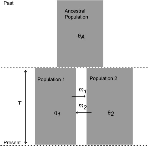
We employ a two-population IM model (Figure 1) and assume selective neutrality. For convenience the two extant populations and the ancestral population are named Pop1, Pop2, and PopA, respectively. For any one population the population size parameter is θ = 4Nu, where N is the effective population size and u is the neutral substitution rate per base pair. The population size parameters for the three populations in the model are denoted as θ₁, θ₂, and θ_A. A migration event from Pop1 to Pop2 (in the coalescent direction, back in time) is represented by M_1→2 and a migration event in the reverse direction is represented by M_2→1. Migration rate parameters have units of migrations per mutation event; i.e., m = M/u, where M is the migration rate per generation. Rates of the two kinds of migration events are denoted as m₁ and m₂, respectively. The speciation time parameter is T = τu, where τ is the time since splitting in generations. In total the model includes six parameters: θ₁, θ₂, θ_A, m₁, m₂, and T.

Figure 1.—

The isolation-with-migration model. The demographic parameters are effective population sizes (θ₁, θ₂, and θ_A), gene migration rates (m₁ and m₂), and population splitting time (T).

One key to integrating over genealogies with migration events is to realize that the probability of the data given the genealogy is unaffected by migration events in the genealogy. This is because Pr(X | G) depends on G only through branching topology and branch lengths. In other words, all genealogies that share the same coalescent events contribute identically to Pr(X | G). Let G* denote a group of genealogies with the same coalescent events (but different migration events). If we can calculate Pr(G* | Θ) together for all genealogies in G*, then

(2)

The new integrand is estimated over the sample space of G*, which is of much lower dimensionality relative to G. Here, we show that for the simple case where only a pair of genes are sampled from two populations, Pr(G* | Θ) can be calculated directly for the IM model.

Coalescent time distribution:

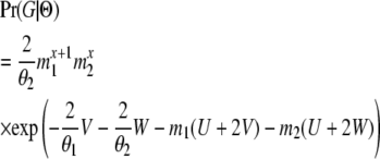
Consider a single locus from which two gene copies are sampled, and consider first the case when one is from Pop1 and the other from Pop2. These two genes coalesce at some time point t. If the coalescent event happened before both genes enter the ancestral population (i.e., t < T), then an odd number (2x + 1, x = 0, 1, 2, …) of migration events must occur before they coalesce, dividing t into 2x + 2 time intervals. During each interval, the ancestral lineages of the two samples reside in one of the three possible states: S₁₁, both ancestral lineages are in Pop1; S₁₂, one ancestral lineage is in Pop1 and the other is in Pop2; and S₂₂, both ancestral lineages are in Pop2.

A migration event will result in a specific switch from one state to another, as shown in Figure 2. A coalescent can happen only in the two states (S₁₁ or S₂₂), when both genes are in the same population. In the event that they coalesce in S₂₂, there will have been 2x + 1 migration events, x + 1 of which are M_1→2 and x of which are M_2→1. Furthermore, of the 2x + 2 time intervals, x + 1 are in state S₁₂, y (0 ≤ y ≤ x) are in state S₁₁, and x − y + 1 are in state S₂₂. We denote the total duration of these three categories of time intervals as U, V, and W (= t − U − V), respectively. Then

(3)

(Beerli and Felsenstein 1999; Hey and Nielsen 2007). Swapping θ₁ with θ₂ and m₁ with m₂ in expression (3) gives the probability of a genealogy in which the coalescent event happens while in state S₁₁.

Figure 2.—

Graphic representation of the three possible states for two sampled genes before coalescence. A migration event will result in a switch from one state to another.

The total probability of a group of genealogies that share the same value for the five variables (x, y, U, V, and W) can be calculated by permutation and convolution,

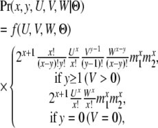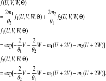
where

(4)

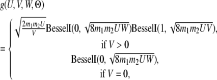
To calculate the total probability of all the genealogies that share the same coalescent time t < T, we need to sum over variables (x, y) and integrate over variables (U, V, W), under the constraint U + V + W = t. The summation can be solved numerically with a closed form,

where

(5)

which leaves

(6)

To the best of our knowledge, there is no analytical solution to the integration in (6). However, this function can be precisely approximated by using numerical integration methods. Note that W = t − U − V, which means that the integration is over two variables instead of three.

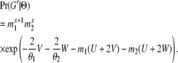
If the coalescent event happens after T, then at time point T both genes are either in the same population (S₁₁ S₂₂) or in different populations (S₁₂). We denote the probability of these two scenarios as Q₀(T, Θ) and Q₁(T, Θ), respectively. For a genealogy with state S₂₂ at time T, let G′ be the part of the genealogy that is more recent than T; then

(7)

Note that (7) differs from (3) only by a factor of and that the constraint is now U + V + W = T. Following the same procedure in (4–6), we get

where

(8)

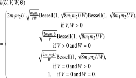
Similarly, we can derive the probability of the state being S₁₂ at time T,

where

(9)

Both Q₀ and Q₁ can be evaluated by numerical integration. And the probability of all genealogies sharing coalescent time t (>T) is

(10)

Note that for both (6) and (10), a swap of parameter θ₁ and m₁ with θ₂ and m₂ does not change the functions. This suggests that the likelihood surface is symmetric and that sampling one sequence from each population will not provide enough resolution for estimating population parameters. Also, in the case when both migration rates are close to zero and each locus is sampled just once from each population, it will not be possible to estimate the size of the sampled populations. To permit estimation of all the parameters in the IM model, we consider the case where two genes are sampled from the same population (either Pop1 or Pop2) at additional loci. The probability of these genealogies can be derived and evaluated in essentially the same way as described above (supporting information, File S1).

A computer program was written to implement an adaptive multidimensional integration routine for the two-dimensional integration in (6) and (10). The adaptive routine estimates a function on a hypercube(s) based on cubature rules, returning an estimate of the integral together with an estimate of the error (Johnson 2005). After each iteration, the routine picks the hypercube with the largest estimated error and divides it into two. The routine stops after the estimated integral converges. Romberg integration (Press et al. 1992) is then used to integrate over t in (2). Both simulated annealing and the downhill simplex method as implemented by Press et al. (1992) are used to search for the maximum-likelihood estimate.

Mutation rate variation:

If it is assumed that all loci have the same mutation rate, then none of the variation that is observed among loci is considered to be caused by variation in the mutation process. We implement this model (identified here as the “single-rate method”) to compare it to models that allow for variation in the mutation rate. In general we expect that methods allowing for variation in mutation rate will be preferable. Failure to account for such variation is expected to lead to an overestimate of the variance in the coalescent process as compensation for the lack of variance in mutation and therefore should introduce bias to the estimates of ancestral population size and species divergence time (Yang 1997).

In an MCMC application of the IM model additional locus-specific mutation scalars are assigned to each locus (Hey and Nielsen 2004). During the MCMC run, these mutation scalars are allowed to vary, subject to the constraint that the product of all scalars equals 1. This approach is effective when multiple sequences are sampled (Hey and Nielsen 2007; Burgess and Yang 2008). However, as our method uses only two gene copies at each locus, there will not be enough information to partition the variation among loci into that due to variance in coalescent times and that due to variance in mutation rates. An alternative method uses the average distance from an outgroup sequence to the sample sequences to calculate a relative mutation rate for each locus (Yang 2002). A problem for this method is that the genealogy of sampled sequences together with the outgroup sequence necessarily shares part of its length with the genealogy for the sampled sequences by themselves. This creates an additional correlation between the outgroup–sample distance and the sample–sample distance and may introduce bias to the parameter estimates. To avoid these issues, we develop two new methods that we identify as “fixed rate” and “all rate” respectively. Both methods rely on sampling an extra pair of sequences, each from an outgroup population, to provide information on mutation rates. When the two chosen outgroup populations have separated from each other for a long time and have not exchanged genes after initial separation, the variance in coalescent time of these two outgroup sequences is small compared to the long population splitting time and can be neglected. Also, the genealogy of the two outgroup sequences is independent of the genealogy of the sampled sequences.

For the fixed-rate method the distance between the two outgroup sequences is used to calculate a fixed mutation scalar for each locus. For example, the mutation scalar of the ith locus (μ_i) is estimated as the outgroup distance (d_i) divided by the average outgroup distance along all loci (),

(11)

These fixed rate scalars are used in the calculation of Pr(X | G) during the search for the maximum likelihood.

Outgroups are also used for the all-rate method, but rather than using them to set fixed mutation rate scalars, the divergence between outgroups for each locus is considered as part of the data. The joint probability of the data is found by assuming a gamma (or uniform) prior, P(μ_i), for the scalars and by integrating over them:

(12)

Here the outgroup distance is represented by X_O and the time of common ancestry of the outgroups is T_O. When an infinite-sites mutation model is applied (Kimura 1969), the integration in (12) can be solved analytically.

Tests on simulated data:

Simulations assuming a single mutation rate:

We tested the performance of the method on two groups of data sets simulated under the six-parameter IM model assuming a single mutation rate for all loci. The first group was simulated under a model of bidirectional migration, with parameter values θ₁ = 0.005, θ₂ = 0.003, θ_A = 0.002, m₁ = 50, m₂ = 100, and T = 0.003. The numerical values for population size and splitting time parameters are much less than one, and the values for the migration rate terms are high because the mutation rate component of these parameters is assumed to be on a per-base pair scale and thus to be quite low. The second group of data sets was simulated without migration, using population parameter values θ₁ = 0.005, θ₂ = 0.003, θ_A = 0.002, m₁ = 0, m₂ = 0, and T = 0.003. These parameter values describe a history in which the divergence time was fairly long ago, relative to population size (i.e., the ratio of the population size parameter to the divergence time parameter is on the order of 1). This means that considerable genetic drift will have occurred following population separation and the majority of genealogies within species are expected to coalesce before the splitting time. To examine how many data the method requires we simulate data sets with different numbers of loci. For each data set, two genes are sampled at each locus from one of three source types: type “12,” where one gene is sampled from each population, and types “11” and “22,” for samples where each gene comes from the same population. We expect loci of the 12 type to provide more information on ancient population history (i.e., θ_A and T) and loci of the 11 and 22 types to provide more information on recent population history (i.e., θ₁ and θ₂). Thus, in addition to varying the total number of sampled loci, we also examined the effect of varying the size of the three categories of samples. In total we simulated data from 9 different sets of category sizes (Table 1). For each combination of population parameter and category size, we simulated 10 data sets. Locus length is fixed at 1000 bp. Data were simulated assuming an infinite-sites mutation model (i.e., all mutations at different points in the sequence) and without recombination, with each locus having an independent coalescent history (i.e., free recombination between loci). A computer program, called SIMDIV, was written to perform the simulations under an IM model.

TABLE 1.

Mean and standard deviation of maximum-likelihood estimates for data sets simulated with uniform mutation rate

	No. of loci			Mean and standard deviation of MLEs
	“11”	“12”	“22”	θ1	θ2	θA	m1	m2	T
I	25	50	25	0.00429 (0.00119)	0.00301 (0.00107)	0.00169 (0.00107)	80.360 (96.111)	100.668 (142.789)	0.00303 (0.00067)
				0.00556 (0.00325)	0.00326 (0.00123)	0.00167 (0.00087)	3.485 (10.092)	19.537 (36.135)	0.00323 (0.00047)
II	250	500	250	0.00556 (0.00074)	0.00297 (0.00045)	0.00205 (0.00024)	43.927 (21.427)	114.992 (46.319)	0.00293 (0.00018)
				0.00491 (0.0004)	0.00300 (0.00022)	0.00191 (0.00019)	2.267 (4.689)	6.393 (16.118)	0.00310 (0.00012)
III	2500	5000	2500	0.00509 (0.00016)	0.00297 (0.00015)	0.00200 (0.00004)	43.111 (6.005)	110.283 (16.236)	0.00300 (0.00003)
				0.00497 (0.00019)	0.00295 (0.00010)	0.00202 (0.00006)	0.257 (0.458)	1.384 (2.598)	0.00299 (0.00003)
IV	25	5000	25	0.00516 (0.00249)	0.00372 (0.00151)	0.00202 (0.00007)	108.132 (56.601)	45.133 (88.054)	0.00299 (0.00005)
				0.00481 (0.00104)	0.00304 (0.00031)	0.00200 (0.00004)	0.966 (1.953)	0.469 (1.351)	0.00302 (0.00003)
V	250	5000	250	0.00488 (0.00069)	0.00299 (0.00052)	0.00200 (0.00006)	39.792 (40.033)	112.329 (57.084)	0.00299 (0.00004)
				0.00504 (0.00045)	0.00291 (0.00016)	0.00196 (0.00006)	1.005 (1.494)	1.284 (3.301)	0.00302 (0.00003)
VI	25	5000	2500	0.00468 (0.00111)	0.00301 (0.00015)	0.00196 (0.00011)	40.232 (16.520)	98.390 (17.358)	0.00302 (0.00006)
				0.00561 (0.0017)	0.00297 (0.00006)	0.00200 (0.00004)	0.209 (0.579)	0.230 (0.719)	0.00301 (0.00002)
VII	250	5000	2500	0.00504 (0.00053)	0.00304 (0.00024)	0.00205 (0.00007)	49.613 (16.590)	100.807 (22.905)	0.00297 (0.00004)
				0.00499 (0.00042)	0.00301 (0.00005)	0.00196 (0.00009)	0.224 (0.490)	0.466 (1.04)	0.00302 (0.00004)
VIII	0	5000	250	0.03352 (0.08029)	0.00297 (0.00077)	0.00201 (0.00003)	62.361 (57.418)	131.58 (97.519)	0.00297 (0.00005)
				0.15932 (0.17869)	0.00299 (0.00025)	0.00200 (0.00007)	0.736 (1.517)	6.212 (10.390)	0.00301 (0.00005)
IX	0	5000	2500	0.08354 (0.15151)	0.00303 (0.00016)	0.00200 (0.00006)	74.678 (46.795)	100.491 (18.893)	0.00299 (0.00006)
				0.10070 (0.18942)	0.00297 (0.00007)	0.00198 (0.00006)	1.397 (2.357)	3.515 (5.334)	0.00303 (0.00003)
True parameters				0.005	0.003	0.002	50	100	0.003
				0.005	0.003	0.002	0	0	0.003

Numbers outside the parentheses are mean MLEs and numbers inside are standard deviations. The top of each cell shows the result from data sets simulated with nonzero migration. The bottom shows the result from data sets simulated without migration.

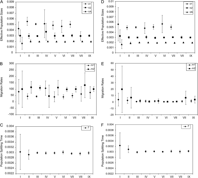
After simulation, each data set was analyzed by searching for the joint maximum-likelihood estimate (MLE) for all six parameters. The precision standard of the numerical integration routines is set at 10⁻⁶ for the log-likelihood of a single locus. This means that for a data set of 10,000 loci, our calculated log-likelihood of the whole data set has an estimated error <0.01. For the 10 data sets simulated under the same parameters and sample sizes, we calculated the mean and standard deviation of the MLEs (Table 1). We also plotted the mean MLEs in Figure 3, with error bars for the standard deviation (SD). For data sets containing no 11 type of loci, we omitted the plots for θ₁ estimates due to their having a very large variance.

Figure 3.—

Maximum-likelihood estimates of population parameters. Symbols in the graph represent the mean maximum-likelihood estimates and bars represent the corresponding standard deviations. I–IX stand for the nine combinations of sample sizes as described in Table 1. Panels (A–C) The result from data sets simulated with nonzero migration. (D–F) The result from data sets simulated without migration.

We analyzed the quality of parameter estimates () using two statistics: bias () and mean square error (MSE) (). Bias is a measure of accuracy, whereas the mean square error reflects both accuracy and precision. Since both statistics are scaled by the true value of the parameter, we omit the calculation when the true value is zero.

Simulations with mutation rate variation:

For each vector of parameter values, 10 data sets were simulated with mutation rate variation. Each data set consisted of 10,000 loci (2500 type 11, 5000 type 12, and 2500 of type 22). A mutation scalar was assigned to each locus at the start of the simulation. These scalars are generated from a Gamma(15, 15) distribution having a mean value of 1. An extra pair of outgroup sequences is simulated at each locus, using the same mutation scalar. The common ancestor time of the two outgroup sequences (T_O) is set to 0.015, which is five times the value for T used in the simulations. Each data set is analyzed using both the fixed-rate and the all-rate methods. For the all-rate method we considered four different prior distributions of mutation rates. First we applied three gamma priors, all with the same mean of 1.0, but with different variances (0.10, 0.67, and 0.05). We also considered a uniform prior (U(0, ∞)). This prior is attractive because it is uninformative; however, it is an improper prior with an infinite mean.

D. melanogaster–D. simulans divergence data:

The genome alignments of D. melanogaster (assembly dm3), D. simulans (assembly droSim1), and D. yakuba (assembly droYak2) were retrieved from the multiple alignments of 15 insect genomes at the UCSC Genome Bioinformatics web site (http://genome.ucsc.edu). The simulans syntenic assembly presents a difficulty because it is the consensus sequence of seven different D. simulans lines and so it is possible for different parts of a locus to be from different lines and to have different evolutionary histories. For this reason D. simulans was represented in our study by genome assemblies from two of the individual inbred lines (w⁵⁰¹ and sim4/6) (Begun et al. 2007). The assumptions of no recombination within loci and free recombination between loci dictate a sampling strategy in which individual loci are sampled as short genomic fragments that are separated from each other by longer stretches. On the basis of findings of the density of apparent recombination events in a previous study using an IM model to study the divergence of Drosophila species (Hey and Nielsen 2004), a length of 500 bp was chosen for sampling loci, with a spacing of at least 2000 bp between loci. Transposons and simple repeats were removed from the data set. Residues next to indels or with a data quality score <40 were discarded to reduce the alignment error and sequencing error. We calculated the six species-pairwise divergence values for each locus and removed loci that showed a smaller outgroup divergence than any “ingroup” divergence [i.e., Min(d_MY, d_SY) ≤ Max(d_MM, d_MS, d_SS)]. Each of the selected loci includes one melanogaster and two simulans sequences (in addition to the outgroup yakuba sequence). Because the calculations are intended for just two gene copies, we randomly picked for each locus two of the three gene copies to go into the data set for analysis. In this way some loci include two simulans sequences and some loci include one simulans and one melanogaster sequence. The final data set included 19,889 MSY (one melanogaster sequence, one simulans sequence, and one yakuba sequence) loci and 10,056 SSY (two simulans sequences and one yakuba sequence) loci.

To include loci with two D. melanogaster sequences, we drew pairs of D. melanogaster sequences from 378 loci studied by Hutter et al. (2007). These D. melanogaster sequences were then each blasted against the melanogaster–simulans–yakuba genome alignment to search for their D. yakuba orthologs. All 378 MMY (two melanogaster sequences and one yakuba sequence) loci passed the data screening procedure described above and were include in the full data set.

RESULTS

Accuracy of estimates:

The means and standard deviations of parameters estimated from simulated data sets are listed in Table 1 and shown in Figure 3. Bias and mean MSE are listed in Table 2. With an input of 10,000 loci distributed across all three types of samples (set III in Table 1 and Figure 3), the method generates estimates that are quite close to the true values of the parameters, with all true values falling in the range of 1 SD away from the mean MLE. For set III simulations the mean MLEs for migration rates have a bias <14% and the mean MLEs for the other parameters all have a bias <2% (Table 2). As expected, the quality of estimates goes down with decreasing total number of loci. For data sets of 1000 loci (set II), the true parameter values still fall within 1 SD of the mean, but with considerably larger MSEs. Similarly for data sets of only 100 loci (set I) the MSEs are much larger, although bias for most parameters is still low. In this case the mean MLEs for m₁ and θ_A have an estimated bias of 60.7% and 14.3%, respectively.

TABLE 2.

Mean square error and bias of maximum-likelihood estimates for data sets simulated with uniform mutation rate

	No. of loci			MSE and bias
	“11”	“12”	“22”	θ1	θ2	θA	m1	m2	T
I	25	50	25	0.0768 (−0.143)	0.1269 (0.003)	0.3123 (−0.155)	4.0636 (0.607)	2.0389 (0.007)	0.0500 (0.011)
				0.4349 (0.111)	0.1768 (0.086)	0.2158 (−0.166)	—	—	0.0304 (0.078)
II	250	500	250	0.0343 (0.111)	0.0227 (−0.009)	0.0154 (0.025)	0.1984 (−0.121)	0.2370 (0.150)	0.0041 (−0.023)
				0.0068 (−0.018)	0.0054 (−0.001)	0.0108 (−0.046)	—	—	0.0027 (0.032)
III	2500	5000	2500	0.0013 (0.018)	0.0025 (−0.011)	0.0003 (0.000)	0.0334 (−0.138)	0.0369 (0.103)	0.0001 (−0.001)
				0.0015 (−0.006)	0.0015 (−0.018)	0.0008 (0.009)	—	—	0.0001 (−0.004)
IV	25	5000	25	0.2487 (0.031)	0.3118 (0.239)	0.0013 (0.008)	2.6332 (1.163)	1.0764 (−0.549)	0.0003 (−0.003)
				0.0449 (−0.039)	0.0112 (0.014)	0.0005 (0.001)	—	—	0.0002 (0.006)
V	250	5000	250	0.0194 (−0.024)	0.0304 (−0.003)	0.0009 (0.001)	0.6827 (−0.204)	0.3411 (0.123)	0.0002 (−0.003)
				0.0081 (0.008)	0.0037 (−0.029)	0.0011 (−0.019)	—	—	0.0001 (0.006)
VI	25	5000	2500	0.0530 (−0.063)	0.0024 (0.004)	0.0031 (−0.018)	0.1473 (−0.195)	0.0304 (−0.016)	0.0005 (0.008)
				0.1310 (0.123)	0.0005 (−0.010)	0.0004 (−0.001)	—	—	0.0001 (0.002)
VII	250	5000	2500	0.0111 (0.008)	0.0065 (0.015)	0.0018 (0.025)	0.1102 (−0.008)	0.0525 (0.008)	0.0003 (−0.010)
				0.0072 (−0.001)	0.0003 (0.003)	0.0024 (−0.021)	—	—	0.0003 (0.007)
VIII	0	5000	250	290.36 (5.704)	0.0657 (−0.009)	0.0003 (0.007)	1.3798 (0.247)	1.0507 (0.316)	0.0004 (−0.011)
				2229.8 (30.86)	0.0070 (−0.003)	0.0013 (0.000)	—	—	0.0003 (0.003)
IX	0	5000	2500	1165.0 (15.71)	0.0029 (0.009)	0.0010 (0.000)	1.1195 (0.494)	0.0357 (0.005)	0.0004 (−0.003)
				1801.5 (19.14)	0.0006 (−0.012)	0.0011 (−0.012)	—	—	0.0002 (0.009)
True parameters				0.005	0.003	0.002	50	100	0.003
				0.005	0.003	0.002	0	0	0.003

Bias and MSE are scaled by the true value of the parameter and its square, respectively. Numbers outside the parentheses are MSE and numbers inside are biases. The top of each cell shows the result from data sets simulated with nonzero migration. The bottom shows the result from data sets simulated without migration.

In addition to the effect of the total number of loci, we see that the quality of parameter estimates depends on the numbers of the three categories of loci. As expected, the estimates of θ_A and T are strongly affected by the number of type 12 loci. When this is set to 5000, the method provides quite accurate estimates for θ_A and T (all biases <2.5% and all MSEs <0.005), even when the data set contains no type 11 loci. We also see that estimates of θ₁ and θ₂ improve quickly with more 11 and 22 types of loci, respectively, and that accurate estimation of m₁ and m₂ requires high numbers of all three types of loci.

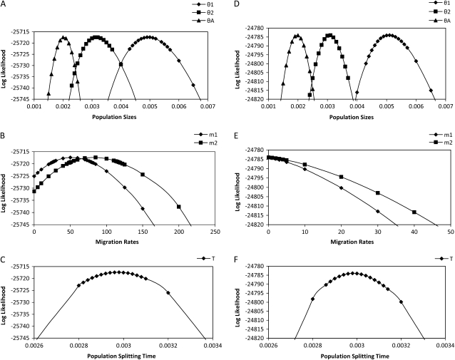
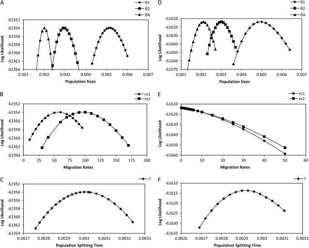
To examine more closely the way that likelihood varies with each parameter we estimated the profile-likelihood function and 95% confidence intervals for each parameter for two randomly picked 10,000-locus data sets. The profile likelihood is the maximized likelihood function conditioned on a selected focal parameter of interest. Figure 4 shows the profile-likelihood curves, and Table 3 shows the 95% confidence intervals (C.I.) calculated from these curves on the basis of the standard assumptions of a likelihood-ratio test. For both parameter sets, all true parameters fall in the range of the 95% C.I., and for data sets simulated with positive migration, we can reject the hypothesis of no migration on the basis of the fact that 0 falls outside of the 95% C.I. for both m₁ and m₂. These curves also reveal some issues that arise for models that include migration. In the first place, the 95% C.I.'s for θ₁, θ₂, θ_A, and T are narrower for data sets simulated without migration. Second, the confidence intervals for m₁ and m₂ are relatively wider than for the other parameters.

Figure 4.—

Profile-likelihood curves for population parameters. (A–C) The result from a data set simulated with nonzero migration. (D–F) The result from a data set simulated without migration.

TABLE 3.

Maximum-likelihood estimate and 95% confidence interval for a data set simulated with a uniform mutation rate

	θ1	θ2	θA	m1	m2	T
True parameters	0.005	0.003	0.002	50	100	0.003
MLE 95% C.I.	0.00496 (0.00455, 0.00537)	0.00314 (0.00287, 0.00346)	0.00202 (0.00188, 0.00216)	51.334 (25.575, 79.317)	83.078 (50.690, 116.563)	0.00298 (0.00287, 0.00308)
True parameters	0.005	0.003	0.002	0	0	0.003
MLE 95% C.I.	0.00508 (0.00479, 0.00539)	0.00307 (0.00292, 0.00323)	0.00198 (0.00186, 0.00211)	0.000 (0.000, 3.021)	0.000 (0.000, 4.512)	0.00298 (0.00292, 0.00305)

The top section shows the result from a data set simulated with nonzero migration. The bottom section shows the result from a data set simulated without migration.

Mutation scalar methods:

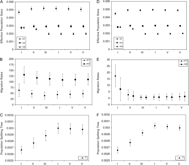
In the simulation studies described above, all data were simulated with a single mutation rate for all loci. However, for real data the substitution rates vary across the chromosome, and neglecting such variance may result in misleading estimates. To address this we analyzed data simulated under a model in which mutation rates were sampled from a Gamma(15, 15) distribution and then analyzed these data under both the fixed-rate method and the all-rate method. Results shown in Table 4 and Figure 5 confirm that neglecting the variance in mutation rates can lead to poor estimation. The single-rate method tends to overestimate migration rates and ancestral population size while underestimating population splitting time and population sizes for sampled populations. As Table 5 shows, estimates generated by the single-rate method have the largest bias. The fixed-rate method generally gives better estimates (smaller bias for all parameters except θ_A) than the single-rate method. However, the fixed-rate method still overestimates ancestral population size and underestimates population splitting time. The all-rate method leads to the most accurate estimates, and it appears that using a gamma prior leads to slightly better results than using the improper uniform prior. It also appears that using different shape/scalar parameters for the gamma prior has only a small effect on the estimation, as all three gamma priors that were considered lead to similar estimates. On the basis of these results the all-rate method is the method of choice.

TABLE 4.

Mean and standard deviation of maximum-likelihood estimates for data sets simulated with varying mutation rate

	Model for mutation scalar	Mean and standard deviation of MLEs
		θ1	θ2	θA	m1	m2	T
I	Single rate	0.00469 (0.00026)	0.00273 (0.00018)	0.00277 (0.00007)	63.669 (28.205)	130.679 (36.067)	0.00267 (0.00006)
		0.00449 (0.00013)	0.00281 (0.00010)	0.00282 (0.00005)	17.384 (8.511)	7.097 (8.940)	0.00266 (0.00005)
II	Fixed rate	0.00512 (0.00023)	0.00292 (0.00018)	0.00258 (0.00011)	47.877 (15.839)	117.302 (27.573)	0.00277 (0.00008)
		0.00493 (0.00012)	0.00297 (0.00007)	0.00260 (0.00005)	2.793 (4.105)	1.775 (3.435)	0.00277 (0.00005)
III	Prior uniform (0, ∞)	0.00519 (0.00023)	0.00291 (0.00018)	0.00200 (0.00013)	39.830 (15.773)	112.995 (27.577)	0.00288 (0.00008)
		0.00490 (0.00011)	0.00293 (0.00008)	0.00197 (0.00006)	0.845 (1.722)	0.568 (1.796)	0.00292 (0.00004)
IV	Prior Gamma (10, 10)	0.00517 (0.00023)	0.00295 (0.00018)	0.00199 (0.00012)	43.978 (15.527)	108.617 (25.925)	0.00300 (0.00008)
		0.00496 (0.00011)	0.00297 (0.00008)	0.00197 (0.00005)	0.884 (1.864)	0.813 (2.530)	0.00303 (0.00004)
V	Prior Gamma (15, 15)	0.00511 (0.00023)	0.00292 (0.00017)	0.00200 (0.00012)	45.486 (14.766)	109.654 (24.792)	0.00299 (0.00008)
		0.00492 (0.00011)	0.00296 (0.00008)	0.00199 (0.00005)	1.105 (2.299)	0.870 (2.697)	0.00302 (0.00004)
VI	Prior Gamma (20, 20)	0.00506 (0.00022)	0.00291 (0.00017)	0.00202 (0.00011)	47.824 (15.430)	110.574 (24.857)	0.00298 (0.00008)
		0.00490 (0.00010)	0.00294 (0.00007)	0.00202 (0.00005)	1.237 (2.645)	1.402 (3.496)	0.00300 (0.00004)
True parameters		0.005	0.003	0.002	50	100	0.003
		0.005	0.003	0.002	0	0	0.003

Numbers outside the parentheses are mean MLEs and numbers inside are standard deviations. The top section of each cell shows the result from data sets simulated with nonzero migration. The bottom section shows the result from data sets simulated without migration.

Figure 5.—

Maximum-likelihood estimates of population parameters. Data are simulated with mutation rates sampled from a Gamma(15, 15) distribution and analyzed using different mutation scalar methods. Symbols in the graph represent the mean maximum-likelihood estimates and bars represent the corresponding standard deviations. I–VI stand for the six different mutation scalar methods as described in Table 4. (A–C) The result from data sets simulated with nonzero migration. (D–F) The result from data sets simulated without migration.

TABLE 5.

Mean square error and bias of maximum-likelihood estimates for data sets simulated with varying mutation rate

	Model for mutation scalar	MSE and bias
		θ1	θ2	θA	m1	m2	T
I	Single rate	0.0064 (−0.061)	0.0118 (−0.091)	0.1496 (0.385)	0.3930 (0.273)	0.2242 (0.307)	0.0128 (−0.111)
		0.0113 (−0.103)	0.0053 (−0.065)	0.1707 (0.412)	—	—	0.0132 (−0.114)
II	Fixed rate	0.0027 (0.023)	0.0045 (−0.028)	0.0870 (0.290)	0.1021 (−0.042)	0.1060 (0.173)	0.0064 (−0.076)
		0.0008 (−0.015)	0.0006 (−0.011)	0.0907 (0.300)	—	—	0.0060 (−0.075)
III	Prior uniform (0, ∞)	0.0037 (0.038)	0.0047 (−0.031)	0.0043 (−0.001)	0.1409 (−0.203)	0.0929 (0.130)	0.0022 (−0.039)
		0.0008 (−0.019)	0.0012 (−0.023)	0.0009 (−0.013)	—	—	0.0008 (−0.026)
IV	Prior Gamma (10, 10)	0.0033 (0.035)	0.0039 (−0.016)	0.0037 (−0.007)	0.1109 (−0.120)	0.0746 (0.086)	0.0007 (0.000)
		0.0005 (−0.008)	0.0007 (−0.008)	0.0009 (−0.014)	—	—	0.0003 (0.011)
V	Prior Gamma (15, 15)	0.0027 (0.023)	0.0040 (−0.027)	0.0034 (0.000)	0.0954 (−0.090)	0.0708 (0.097)	0.0007 (−0.003)
		0.0007 (−0.015)	0.0008 (−0.013)	0.0007 (−0.006)	—	—	0.0002 (0.006)
VI	Prior Gamma (20, 20)	0.0020 (0.012)	0.0043 (−0.031)	0.0032 (0.010)	0.0971 (−0.044)	0.0730 (0.106)	0.0007 (−0.006)
		0.0009 (−0.021)	0.0010 (−0.019)	0.0008 (0.011)	—	—	0.0002 (0.000)
True parameters		0.005	0.003	0.002	50	100	0.003
		0.005	0.003	0.002	0	0	0.003

Bias and MSE are scaled by the true value of the parameter and its square, respectively. Data are simulated with mutation rate variation and analyzed using different mutation scalar methods. Numbers outside the parentheses are MSE and numbers inside are biases. The top of each cell shows the result from data sets simulated with nonzero migration. The bottom shows the result from data sets simulated without migration.

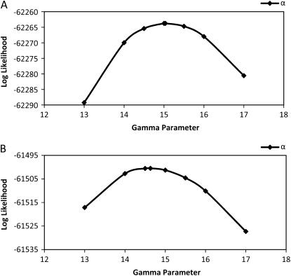
We also looked at profile likelihoods for a small sample of data sets simulated with mutation rate variation and analyzed using the all-rate method with a gamma(15, 15) prior. Figure 6 shows the profile-likelihood curves, and from these the 95% confidence intervals (Table 6) were calculated as described above. For the all-rate method, all true parameter values fall in the range of the 95% C.I. For the data set simulated with nonzero migration, we can reject the hypothesis of no migration because 0 falls out of the 95% C.I. for both m₁ and m₂. The profile likelihood for the shape/scale parameter of the gamma prior is shown in Figure 7, and we note that the estimated MLE for the gamma prior is close to the true value of 15 used in the simulations.

Figure 6.—

Profile-likelihood curves for population parameters. Data are simulated with mutation rate variation and analyzed using a all-rate model with a Gamma(15, 15) prior. (A–C) The result from a data set simulated with nonzero migration. (D–F) The result from a data set simulated without migration.

TABLE 6.

Maximum-likelihood estimate and 95% confidence interval for a data set simulated with varying mutation rate

	θ1	θ2	θA	m1	m2	T
True parameters	0.005	0.003	0.002	50	100	0.003
MLE 95% C.I.	0.00520 (0.00479, 0.00565)	0.00295 (0.00269, 0.00324)	0.002 (0.-2, 0.00215)	52.898 (28.592, 81.430)	97.784 (64.305, 131.988)	0.00301 (0.00290, 0.00314)
True parameters	0.005	0.003	0.002	0	0	0.003
MLE 95% C.I.	0.00497 (0.00471, 0.00527)	0.00300 (0.00286, 0.00315)	0.00207 (0.00194, 0.00221)	0.000 (0.000, 3.651)	0.000 (0.000, 3.551)	0.00294 (0.00286, 0.00331)

Data are simulated with mutation rate variation and analyzed using a all-rate model with a Gamma(15, 15) prior. The top section shows the result from a data set simulated with nonzero migration. The bottom section shows the result from a data set simulated without migration. Both data sets are simulated with mutation rate variation.

Figure 7.—

Profile-likelihood curves for the gamma parameter of the mutation scalar prior. (A) The curve from a data set simulated with nonzero migration. (B) The curve from a data set simulated without migration.

Application to Drosophila divergence:

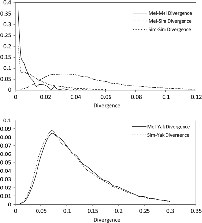
The melanogaster–simulans divergence data include a total of 30,323 loci, with an average length of 405 bp. Figure 8 shows the distributions of five measures of divergence calculated from the data. The average divergence between a pair of melanogaster sequences (0.00587) is smaller than the average divergence between a pair of simulans sequences (0.01323), suggesting that D. simulans has a larger effective population size than D. melanogaster. The average divergence between melanogaster sequence and simulans sequence is 0.04387 and the average melanogaster–yakuba and simulans–yakuba divergences are 0.11566 and 0.11048, respectively. For divergence of this magnitude, the chance of multiple mutations per base position cannot be neglected. Therefore, we adopted the JC69 mutation model instead of the infinite-site model. Because the all-rate method can be used only with the infinite-site model, we use the second-best method (fixed-rate method) to account for the mutation rate variation. Also, due to the fact that only one outgroup sequence is available, we calculate the mutation scalars based on melanogaster-yakuba divergence, instead of using a pair of outgroup sequences.

Figure 8.—

Distribution curves of divergence. (Top) Solid line, dashed line, and dashed-dotted line represent distribution of melanogaster–melanogaster, simulans–simulans, and melanogaster–simulans divergence, respectively. (Bottom) Solid line and dashed line represent distribution of melanogaster–yakuba and simulans–yakuba divergence, respectively.

The maximum-likelihood estimates for the isolation-with-migration model are listed in Table 7. The estimated melanogaster effective population size is 0.00552. The estimated simulans population size (0.01352) is ∼2.4 times the estimated melanogaster population size, in agreement with several previous studies. (Hey and Kliman 1993; Moriyama and Powell 1996) The estimated ancestral population size is 0.00691, slightly bigger than the melanogaster population size. A nonzero simulans-to-melanogaster (melanogaster-to-simulans if looking backward in time) migration rate is estimated. We test the significance of this gene flow by comparing the log-likelihood of MLEs from the isolation-with-migration and a model with zero gene flow (i.e., the isolation model). Let Λ be the difference between two log-likelihood values. Had the real migration rates been zero, we would expect −2Λ to follow a composite χ²-distribution (0.25 + 0.5 + 0.25) (Hey and Nielsen 2007). In our case, −2Λ = 1535.64, which far exceeds typical significance criteria (i.e., P ≪ 0.001), and we therefore reject the isolation model.

TABLE 7.

Population parameters estimated for melanogaster–simulans divergence

Model, data	θ1	θ2	θA	m1	m2	T	Log-likelihood
IM, full length	0.00552	0.01352	0.00691	4.846	0.000	0.01715	−1904163.35
Isolation, full length	0.00585	0.01352	0.00845	0.000	0.000	0.01583	−1904931.17
IM, half length	0.00513	0.01328	0.00837	6.820	0.000	0.01688	−937386.51
Isolation, half length	0.00560	0.01328	0.01035	0.000	0.000	0.01507	−937907.78
Divergence filter	θ1	θ2	θA	m1	m2	T
Upper 2%	0.00542	0.01301	0.00673	3.848	0.000	0.01711
Upper and lower 2%	0.00535	0.01305	0.00676	3.018	0.000	0.01713
Converted parameter	N1 (106)	N2 (106)	NA (106)	2N1M1 (10−2)	2N2M2 (10−2)	T′ (MYA)
IM, full length	2.44 (2.18, 2.77)	5.99 (5.85, 6.12)	3.06 (2.97, 3.15)	1.34 (1.06, 1.69)	0.00 (0.00, 0.00)	3.04 (3.02, 3.06)

Our method assumes that no recombination happened within each locus during the time since its time to the most recent common ancestor (TMRCA). To assess the impact of recombination events on our estimates, we generated a new data set by taking the first half of the sequence from each locus. The new data set has a shorter average length of 203 bp and is therefore less likely to have experienced recombination in the time since the TMRCA. Parameter estimates for the “half-length” data set are similar to those for the “full-length” data set (Table 7). Only small differences are detected between the estimates for current population sizes and speciation time, and the effective ancestral population size and simulans-to-melanogaster migration rate estimates from half-length data are ∼30% larger than those from the full-length data, suggesting possible negative biases introduced by recombination. As in the case of the full-length data set, the gene flow parameter from simulans to melanogaster in the half-length data is statistically significant (−2Λ = 1042.54, P ≪ 0.001).

Another possible concern is that a subset of the loci included in the study might be in error (e.g., by sequencing or alignment error) and that these could shift the distribution of divergence values in such a way as to create a signal of gene flow. To investigate this possibility, we generated two more filtered data sets by removing loci with extreme values for divergence. First we removed all the loci from the original data set that fall in the top 2% of any of the divergence distributions (i.e., melanogaster–simulans, melanogaster–melanogaster, simulans–simulans, or melanogaster–yakuba divergence). A total of 28,881 loci remain in this first filtered data set. Then a second filtered data set was generated from the first filtered data set by removing loci falling in the bottom 2% of either the melanogaster–simulans or the melanogaster–yakuba divergence distribution. The second filtered data set includes 27,636 loci. Estimates for effective population sizes and speciation time from these two filtered data sets are very close to those from original data while estimates for simulans-to-melanogaster migration rate are only slightly smaller (Table 7). While these contrasts do not completely remove the possibility that errors in the data contribute to the estimates, they do suggest that the parameter estimates and the finding of significant gene flow do not depend strongly on the tails of the divergence distributions.

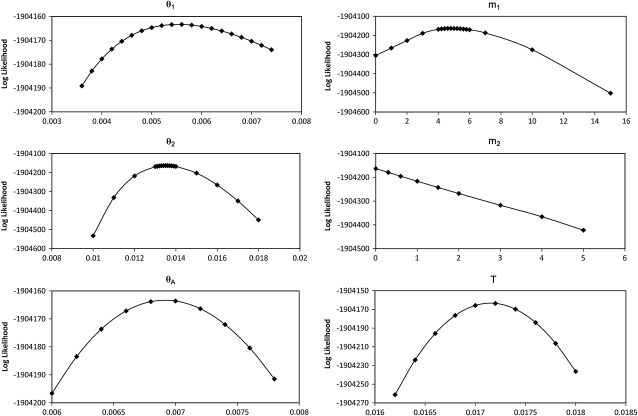
We estimated the 95% confidence intervals of the six parameters from their profile-likelihood curves (Figure 9). Both MLEs and 95% C.I.'s were then converted to their conventional forms, using 10-million-year melanogaster–yakuba speciation time as the calibration point and 0.1 year as the generation time (Powell 1997). The effective population sizes for melanogaster, simulans, and their ancestral population, after conversion, are 2.44, 5.99, and 3.06 million, respectively. The melanogaster–simulans speciation time is estimated at 3.04 million years ago (MYA), and the population migration rate from simulans to melanogaster (2N₁M₁) is estimated at 0.0134 migrant gene copies per generation.

Figure 9.—

Profile-likelihood curve for population parameters estimated from melanogaster–simulans–yakuba genome alignment.

DISCUSSION

We describe a new likelihood-based inference method for the isolation-with-migration model. This method resembles Yang's (2002) by using numerical integration to evaluate the likelihood function, and consequently both our method and Yang's share the same limitation in that they cannot handle data with large samples at each locus. However, they can handle data from many independently segregating loci. The situation raises the question of just how sampling effort should be proportioned: More loci with few gene copies each? Or fewer loci with more gene copies per locus?

In 2006, Felsenstein studied the accuracy of maximum-likelihood estimates of effective population size for a single population (Felsenstein 2006). Using simulated data he found the accuracies of the MLE were well predicted by the formula developed by Fu and Li (1993). According to that formula, the accuracy of the estimation is proportional to the number of loci and approximately proportional to the logarithm of the number of sampled genes at each locus. This result agrees with the conclusion of Pluzhnikov and Donnelly (1996) that it is optimal to take small samples from populations. Felsenstein noted that this is because the increase in total branch length by sampling extra sequences goes down as the sample size becomes bigger. Although Felsenstein's study was performed on only a single population, the reasoning can be extended to the case of the IM model, especially when the population splitting time is long compared to both extant population sizes and when migration rates are not high. Under this scenario, two samples from the same population will most likely coalesce before they either enter the ancestral population or migrate into the other population. Thus, estimating the effective population size of a sampled population is similar to the case of estimating the size of a single population, favoring samples with a large number of loci with two gene copies from the population for which the size parameter is to be estimated.

The estimates for ancestral population size and population splitting time depend primarily on samples from different populations, in which case they coalesce only after they enter the ancestral population or after one of them migrates into the other population. This process may take a long time unless migration is high. When additional samples are collected, they tend to coalesce with genes from the same population and contribute little to the length of the genealogy. Since the estimation of ancestral population size and population splitting time relies on old coalescent history, it appears that it is better to have a large number of loci with one sample from each population.

Estimating migration rates also benefits from more loci with one sample from each population, because longer branches are more likely to carry migration events. However, the occurrences of migration events can be detected only if two samples from different populations coalesce before entering the ancestral population. This means that it is not possible to estimate migration rates well without also estimating population sizes well. Therefore, to achieve good estimates for migration rates, it is preferable to have multiple loci from all three sampling schemes (i.e., some with two sequences from one population, some with two from the other population, and some with one from each). This is in agreement with our results from simulation data.

A common question in statistical population genetics is, How much of the variation that is observed among loci is due to variation in the actual mutation rate? Some methods assume that there is no uncertainty in outgroup-based mutation rate estimates (Becquet and Przeworski 2007) or that all base positions have the same mutation rate (Innan and Watanabe 2006). For data that match either of these assumptions, our method, using the single-rate assumption, performs quite well (Figure 3). The problem, however, for such methods that assume no mutation rate variation, is that when they are applied to real data that do vary in mutation rate, the additional variance will be attributed to variance in the coalescent process.

For data that do come from loci that vary in their substitution rates, the question arises of how best to use information from outgroup species to account for this variation. If outgroup populations have been separated for enough time, the variance in the coalescent process may be ignored and the expected outgroup divergence is proportional to the substitution rate. Thus one direct way to estimate a relative mutation scalar for a locus is to use the observed outgroup divergence at that locus. However, even if we assume that there is no variation due to the coalescent in the outgroup divergence, the variance of outgroup divergence still includes both a variance among mutation rates and a stochastic variance of the mutation process. By using a fixed mutation scalar derived from the outgroup divergence we are in effect treating all of the variance in outgroup divergence as being due to mutation rate variation. For the purpose of illustration, assume there is actually no variation in mutation rate among loci. Under these circumstances some loci will still have larger (or smaller) outgroup divergence due to random variation in the mutation process, and this variation will be interpreted as variation in mutation rates. When variable fixed rates that were actually sampled from a process with no mutation rate variation are applied to the model, the introduced variation leads to additional variation in the coalescent times. We identify this effect of overestimating the variance in sample coalescent time as “overcompensation.” As a result of overcompensation we expect to overestimate ancestral population size and to underestimate population splitting time. These biases are in agreement with our results on simulated data (Table 4 and Figure 5). Burgess and Yang (2008) also found similar trends in their study.

An alternative to using a fixed mutation rate for each locus, based on outgroup divergence, is to treat the mutation scalar as a random variable. In this method we consider outgroup divergence as part of the data, and the joint likelihood of sample divergence and outgroup divergence is integrated over a prior distribution for the mutation scalar. This is equivalent to integrating the likelihood function over the posterior distribution of the mutation scalar that is derived from outgroup divergence. Our analyses with this all-rate method, and a prior gamma distribution, yielded estimates with the least bias, compared to results for other ways of handling the mutation rate scalars. We also observed little sensitivity of estimates to the choice of the gamma distribution parameter.

The method described here is designed for data sets with very small samples for very large numbers of loci. Specifically it can be applied in cases where data are available from two genomes, from each of two closely related species. As DNA sequencing techniques advance, we can anticipate growing availability of multiple whole-genome sequences for pairs of recently diverged species. Although we do not yet have two genome sequences from each of two closely related species, we can anticipate some of the issues that will arise when preparing the data for analysis. One large issue is the choice of outgroup species, which need to have been separated for a relatively long time, so that the ancestral polymorphism is small compared to divergence. On the other hand, these populations should not be too far away from the populations under study to guard against the possibility of not sharing actual mutation rates.

Two other key issues are recombination and selection. Our method follows basic coalescent theory by assuming selective neutrality, no recombination within loci, and free recombination between loci. Violation of these assumptions will impair the validity of the analysis and bring bias to the estimates. Preferably loci that have undergone directional or balancing selection, or recombination since the TMRCA, during the divergence process, should be removed from the input data. When multiple (≥2) genome sequences from each population are available, several statistical tests are available for screening for possible selection events, either by comparing nonsynonymous and synonymous substitutions [d_N/d_S test (Li et al. 1985)] or by comparing polymorphism and divergence (the HKA test of Hudson et al. 1987). To guard against within-locus recombination, we suggest using short sequences. We also suggest that sequences be taken from genome locations that are separated by a sufficient distance so that their evolutionary histories are effectively independent of each other.

Drosophila divergence:

To demonstrate the method with real data we studied the divergence process of D. simulans and D. melanogaster. The estimated effective population size of D. melanogaster is 2.44 × 10⁶, which is similar to the estimated values of 2.4 × 10⁶ by Thornton and Andolfatto (2006) and 3 × 10⁶ by Li et al. (1999). The estimated speciation time between is 3.04 MYA, which is somewhat larger than the 2.3-MYA estimate of Li et al. (1999). We also estimated that the divergence history included gene flow in the direction from D. simulans to D. melanogaster. The estimated population migration rate, 0.0134 migrations per generation, is ≪1 and therefore would have little impact on the rate of divergence by genetic drift (Wright 1931). However, neglecting this weak gene flow would still lead to an overestimate of the ancestral population size and underestimating the speciation time (Table 7), a point that nicely highlights the advantage of using a demographic model that incorporates migration.

References

- Becquet, C., and M. Przeworski, 2007. A new approach to estimate parameters of speciation models with application to apes. Genome Res. 17 1505–1519. [DOI] [PMC free article] [PubMed] [Google Scholar]
- Beerli, P., and J. Felsenstein, 1999. Maximum-likelihood estimation of migration rates and effective population numbers in two populations using a coalescent approach. Genetics 152 763–773. [DOI] [PMC free article] [PubMed] [Google Scholar]
- Beerli, P., and J. Felsenstein, 2001. Maximum likelihood estimation of a migration matrix and effective population sizes in n subpopulations by using a coalescent approach. Proc. Natl. Acad. Sci. USA 98 4563–4568. [DOI] [PMC free article] [PubMed] [Google Scholar]
- Begun, D. J., A. K. Holloway, K. Stevens, L. W. Hillier, Y. P. Poh et al., 2007. Population genomics: whole-genome analysis of polymorphism and divergence in Drosophila simulans. PLoS Biol. 5 e310. [DOI] [PMC free article] [PubMed] [Google Scholar]
- Burgess, R., and Z. Yang, 2008. Estimation of hominoid ancestral population sizes under Bayesian coalescent models incorporating mutation rate variation and sequencing errors. Mol. Biol. Evol. 25 1979–1994. [DOI] [PubMed] [Google Scholar]
- Felsenstein, J., 1988. Phylogenies from molecular sequences: inference and reliability. Annu. Rev. Genet. 22 521–565. [DOI] [PubMed] [Google Scholar]
- Felsenstein, J., 2006. Accuracy of coalescent likelihood estimates: Do we need more sites, more sequences, or more loci? Mol. Biol. Evol. 23 691–700. [DOI] [PubMed] [Google Scholar]
- Fu, Y. X., and W. H. Li, 1993. Statistical tests of neutrality of mutations. Genetics 133 693–709. [DOI] [PMC free article] [PubMed] [Google Scholar]
- Griffiths, R. C., and P. Marjoram, 1996. Ancestral inference from samples of DNA sequences with recombination. J. Comput. Biol. 3 479–502. [DOI] [PubMed] [Google Scholar]
- Hey, J., and R. M. Kliman, 1993. Population genetics and phylogenetics of DNA sequence variation at multiple loci within the Drosophila melanogaster species complex. Mol. Biol. Evol. 10 804–822. [DOI] [PubMed] [Google Scholar]
- Hey, J., and R. Nielsen, 2004. Multilocus methods for estimating population sizes, migration rates and divergence time, with applications to the divergence of Drosophila pseudoobscura and D. persimilis. Genetics 167 747–760. [DOI] [PMC free article] [PubMed] [Google Scholar]
- Hey, J., and R. Nielsen, 2007. Integration within the Felsenstein equation for improved Markov chain Monte Carlo methods in population genetics. Proc. Natl. Acad. Sci. USA 104 2785–2790. [DOI] [PMC free article] [PubMed] [Google Scholar]
- Hudson, R. R., M. Kreitman and M. Aguade, 1987. A test of neutral molecular evolution based on nucleotide data. Genetics 116 153–159. [DOI] [PMC free article] [PubMed] [Google Scholar]
- Hutter, S., H. Li, S. Beisswanger, D. De Lorenzo and W. Stephan, 2007. Distinctly different sex ratios in African and European populations of Drosophila melanogaster inferred from chromosomewide single nucleotide polymorphism data. Genetics 177 469–480. [DOI] [PMC free article] [PubMed] [Google Scholar]
- Innan, H., and H. Watanabe, 2006. The effect of gene flow on the coalescent time in the human-chimpanzee ancestral population. Mol. Biol. Evol. 23 1040–1047. [DOI] [PubMed] [Google Scholar]
- Johnson, S. G., 2005. Adaptint.c, GNU Scientific Library Extensions. http://www.gnu.org/software/gsl.
- Kimura, M., 1969. The number of heterozygous nucleotide sites maintained in a finite population due to steady flux of mutations. Genetics 61 893–903. [DOI] [PMC free article] [PubMed] [Google Scholar]
- Kuhner, M. K., J. Yamato and J. Felsenstein, 1995. Estimating effective population size and mutation rate from sequence data using Metropolis-Hastings sampling. Genetics 140 1421–1430. [DOI] [PMC free article] [PubMed] [Google Scholar]
- Li, W. H., C. I. Wu and C. C. Luo, 1985. A new method for estimating synonymous and nonsynonymous rates of nucleotide substitution considering the relative likelihood of nucleotide and codon changes. Mol. Biol. Evol. 2 150–174. [DOI] [PubMed] [Google Scholar]
- Li, Y. J., Y. Satta and N. Takahata, 1999. Paleo-demography of the Drosophila melanogaster subgroup: application of the maximum likelihood method. Genes Genet. Syst. 74 117–127. [DOI] [PubMed] [Google Scholar]
- Moriyama, E. N., and J. R. Powell, 1996. Intraspecific nuclear DNA variation in Drosophila. Mol. Biol. Evol. 13 261–277. [DOI] [PubMed] [Google Scholar]
- Nielsen, R., and J. Wakeley, 2001. Distinguishing migration from isolation: a Markov chain Monte Carlo approach. Genetics 158 885–896. [DOI] [PMC free article] [PubMed] [Google Scholar]
- Pluzhnikov, A., and P. Donnelly, 1996. Optimal sequencing strategies for surveying molecular genetic diversity. Genetics 144 1247–1262. [DOI] [PMC free article] [PubMed] [Google Scholar]
- Powell, J. R., 1997. Progress and Prospects in Evolutionary Biology: The Drosophila Model. Oxford University Press, London/New York/Oxford.
- Press, W. H., S. A. Teukolsky, W. T. Vetterling and B. P. Flannery, 1992. Numerical Recipes in C—The Art of Scientific Computing. Cambridge University Press, Cambridge, UK.
- Thornton, K., and P. Andolfatto, 2006. Approximate Bayesian inference reveals evidence for a recent, severe bottleneck in a Netherlands population of Drosophila melanogaster. Genetics 172 1607–1619. [DOI] [PMC free article] [PubMed] [Google Scholar]
- Wilson, I. J., and D. J. Balding, 1998. Genealogical inference from microsatellite data. Genetics 150 499–510. [DOI] [PMC free article] [PubMed] [Google Scholar]
- Wright, S., 1931. Evolution in Mendelian populations. Genetics 16 97–159. [DOI] [PMC free article] [PubMed] [Google Scholar]
- Yang, Z., 1997. On the estimation of ancestral population sizes of modern humans. Genet. Res. 69 111–116. [DOI] [PubMed] [Google Scholar]
- Yang, Z., 2002. Likelihood and Bayes estimation of ancestral population sizes in hominoids using data from multiple loci. Genetics 162 1811–1823. [DOI] [PMC free article] [PubMed] [Google Scholar]