Relationship between threshold and suprathreshold perception of position and stereoscopic depth

Abstract

We seek to determine the relationship between threshold and suprathreshold perception for position offset and stereoscopic depth perception under conditions that elevate their respective thresholds. Two threshold-elevating conditions were used: (1) increasing the interline gap and (2) dioptric blur. Although increasing the interline gap increases position (Vernier) offset and stereoscopic disparity thresholds substantially, the perception of suprathreshold position offset and stereoscopic depth remains unchanged. Perception of suprathreshold position offset also remains unchanged when the Vernier threshold is elevated by dioptric blur. We show that such normalization of suprathreshold position offset can be attributed to the topographical-map-based encoding of position. On the other hand, dioptric blur increases the stereoscopic disparity thresholds and reduces the perceived suprathreshold stereoscopic depth, which can be accounted for by a disparity-computation model in which the activities of absolute disparity encoders are multiplied by a Gaussian weighting function that is centered on the horopter. Overall, the statement “equal suprathreshold perception occurs in threshold-elevated and unelevated conditions when the stimuli are equally above their corresponding thresholds” describes the results better than the statement “suprathreshold stimuli are perceived as equal when they are equal multiples of their respective threshold values.”

1. INTRODUCTION

Perceptual thresholds exist in all sensory modalities including vision and are commonly measured using psychophysical methods. Within the visual system, various subsystems (motion, color, etc.) exhibit their own thresholds. There are two possible interpretations of the threshold. In one model called the high-threshold model [1], a behavioral response is generated by a physical stimulus via two sequential processes: (a) a sensory process and (b) a decision process. In this model, threshold is defined as the minimum level of physical stimulus that can generate an output from the sensory process. When the physical stimulus is equal to the sensory threshold, the behavioral response is at a chance level. In a second model called the signal detection model [2], there are still the same two processes, but a sensory threshold does not exist. The output of the sensory process is continuous but is assumed to be noisy. The behavioral response is generated based on the noisy output of the sensory process and a decision criterion. Threshold in the signal detection model is defined as the physical stimulus that yields a criterion level of performance. Regardless of which model one uses, the threshold is an important parameter of any visual subsystem because it determines the smallest input signal needed to generate a reliable perceptual output.

Numerous psychophysical studies have documented how the thresholds for various visual functions depend on (1) aspects of the stimulus, such as luminance, contrast, and retinal location, and (2) characteristics of the observer, such as age, refractive error, and fixation stability. Although it is well established that visual thresholds are elevated substantially under conditions such as low luminance, reduced contrast, and image blur, it is much less clear how these conditions affect the perception of suprathreshold visual stimuli. For example, if the threshold for stereoscopic depth is elevated fivefold by a given amount of image blur, to what extent does the same amount of blur attenuate the depth that is perceived from suprathreshold binocular image disparities?

Despite large differences between the contrast thresholds for patterns of different spatial and temporal frequency, the perception of suprathreshold spatial [3,4] and temporal contrast [5] is known to be approximately veridical. These results imply that the perception of suprathreshold contrast is largely compensated, or “normalized,” for the substantial spatiotemporal frequency variation in contrast thresholds. Schor and Wood [6] showed that the relative stereoscopic disparity threshold (stereothreshold) for narrowband stimuli also depends on spatial frequency. In particular, stereothresholds are elevated if the center spatial frequency of the stimulus is reduced below ~2.5 cycles per degree (cpd). However, unlike the reported results for contrast perception, our analysis of the data in [6] indicates that the perceived magnitude of suprathreshold depth is systematically in error for low spatial frequency stimuli. When considered in conjunction with the data on contrast “normalization” [3,5,7,8], these results suggest that the relationship between threshold and suprathreshold perception may depend on the specific visual function under consideration. As psychophysical thresholds can be elevated by a wide variety of parameters, it is also possible that the relationship between threshold and suprathreshold perception within a subsystem depends on the condition (i.e., the stimulus parameters) under which the threshold is measured.

One of the reasons it is important to study the relationship between threshold and suprathreshold perception is because the degradation of a visual function is quantified typically by the elevation of related threshold (e.g., visual acuity quantifies the image degradation produced by the eye’s optics). The impact that a threshold elevation has on visual performance and the quality of life of an observer can be gauged only by examining the responses of the degraded system to a full range of inputs, from near threshold to substantially suprathreshold levels. This is because most of the stimuli encountered in natural viewing are suprathreshold. An important theoretical reason to evaluate suprathreshold as well as threshold perception is that the properties of an arbitrary system, normal or degraded, can be characterized fully only by studying its output in response to the full range of inputs. Unlike a linear system, which is characterized completely by determining the output due to a single input (i.e., an impulse), most visual subsystems are nonlinear.

In this study, we addressed three questions about the relationship between threshold and suprathreshold visual perception. First, is the phenomenon of suprathreshold normalization ubiquitous among visual functions? Second, does suprathreshold normalization in a threshold-elevating condition depend on the condition that causes the threshold elevation? And third, how is suprathreshold perception related quantitatively to the threshold? To address these questions, we measured threshold and suprathreshold perception for two visual subsystems that process (1) relative position and (2) stereoscopic depth. For each subsystem, we measured threshold and suprathreshold perception for two threshold-elevating conditions: (a) interstimulus gap [9,10] and (b) blur [11–13]. In the gap condition, thresholds were elevated by increasing the separation (or gap) between the two lines that compose the stimulus (see Fig. 1). In the blur condition, thresholds were elevated by adding 2 D of dioptric blur to the stimulus. Suprathreshold perception was measured using a matching paradigm. We found that the perception of suprathreshold position (Vernier) offset and stereoscopic depth from relative disparity remain veridical when thresholds were elevated up to a factor of 10 times by increasing the interline gap. The perception of suprathreshold position offset also remains veridical when the Vernier threshold is elevated by dioptric blur. In contrast, perceived suprathreshold stereoscopic depth is reduced systematically in the presence of dioptric blur.

Fig. 1.

(a) For the stimuli used in the position-offset experiments (top), the horizontal distance p between the vertical dotted lines is defined as the Vernier offset. In the fused percept (bottom), the observer sees the bottom line shifted rightward relative to the top line, with both lines in the same depth plane. (b) The stimuli used in the stereoscopic depth experiments (top) differed from those in (a) in that opposite directions of monocular offsets were presented to each eye to generate stereoscopic disparity. Twice the horizontal distance between the vertical dotted lines (2p) is defined as the relative stereoscopic disparity. In the fused percept (bottom), the observer sees the bottom line in front of (or behind) the top line, with both lines in the same perceived direction.

Last, we tested several descriptive models to mathematically relate suprathreshold perception of position offset and stereoscopic depth to their respective thresholds. Overall, we found that our data are explained better by a model proposed previously by Kulikowski [8] to account for contrast normalization than by “proportional” models based on Stevens’s and Weber–Fechner’s laws. In an attempt to relate our data to known neural mechanisms that underlie the processing of visual position and stereoscopic depth, we determined that (a) perception of suprathreshold relative position offset in threshold-elevating conditions can be autonormalized by a topographical-map-based encoding of position information, and (b) the perception of suprathreshold stereoscopic depth in the presence of dioptric blur can be accounted for by a mechanism that weighs the activity in a population of disparity encoders by a Gaussian function that is centered on the horopter.

2. METHODS

The stimulus configurations used in the position-offset and stereoscopic depth experiments are shown in Figs. 1(a) and 1(b), respectively. The fused binocular stimulus was a pair of bright vertical lines separated vertically by an interline gap. The dimensions of each line were 30′ by 0.2′. It should be pointed out that the width of the line on the retina is expected to be approximately 1′ because of the aberrations of the eye. The stimulus was viewed from 395 cm through a mirror haploscope using matched pairs of polarizing filters in front of the eyes and in front of each half of a display oscilloscope (Hewlett Packard 1311B). The bright lines (30 cd/m² when viewed through matching polarizing filters) were presented on a dark background at a 240 Hz refresh rate. Vernier position offset and relative stereoscopic disparity were introduced by horizontally shifting the bottom line in the image presented to each eye. Based on the direction of the position offset (same or opposite) in the two eyes, the observers perceived the bottom line either to be displaced laterally [same direction; Fig. 1(a)] or to be in a different depth plane (opposite direction; [Fig. 1(b)] compared with the top line.

We used two conditions to elevate the threshold for Vernier offset and stereoscopic depth: (1) an increase in the inter-line gap and (2) the introduction of dioptric blur. Two types of experiments were conducted for each condition: (a) a threshold experiment to determine the Vernier or relative stereoscopic disparity threshold, and (b) a suprathreshold experiment to match perceived suprathreshold position offsets or stereoscopic depth. These experiments are described below in greater detail. Either four (in the gap condition) or three observers (in the blur condition) with corrected visual acuity of 20/20 or better and normal binocular vision participated in the experiments, after voluntarily granting informed consent.

A. Gap Condition

1. Position-Offset Experiments

Using the stimulus configuration represented in Fig. 1(a), position-offset (Vernier) thresholds were measured for interline gaps of 10′ (20′ for observer S2) and 100′ (720′ for observer S2) in separate sessions. The larger range of interline gaps used for observer S2 was achieved by decreasing the viewing distance of the targets. The method of constant stimuli was used to measure thresholds. A bright fixation cross remained on the oscilloscope until the observer initiated each trial by pressing a joystick button. Upon initiation of the trial, the fixation cross disappeared, and, after a delay of 200 ms, a Vernier target was presented for 200 ms. The delay was introduced to minimize the possibility that the short-duration Vernier stimulus would be masked by the transient at fixation offset. The observer was instructed to maintain fixation and not make an eye movement. The horizontal position offset between the upper and lower line targets was selected randomly from an array of seven preset offsets. The observer indicated the direction of the position offset (left or right) using the joystick. Each offset in the array was presented 10 times. A psychometric function was fit to the data for each block of 70 trials using probit analysis. The threshold corresponds to the inverse slope of the psychometric function (50 to 84% range) averaged across two to three replications.

In the experiment to match perceived suprathreshold position offset, a bright fixation cross again was visible until the observer initiated each trial. The fixation cross then disappeared and, after a delay of 200 ms, the test stimulus [gap=100′ except observer S2’s gap=720′; see Fig. 1(a)] was presented for 200 ms with a horizontal position offset. Within each block of trials, the position offset of the test stimulus remained constant. For each observer, the offset was selected from a predetermined set of offsets that represented specific multiples of the observer’s position-offset threshold for this stimulus configuration, e.g., ±2X, ±4X, etc., where the negative and positive signs indicate that the bottom line was offset to the left or right, respectively, of the top line. For observer S2, the maximum offset of the test stimulus was ±12 times his Vernier position-offset threshold. After the test stimulus disappeared, the fixation cross was immediately redisplayed for 2 s and was then extinguished again. After another 200 ms delay, the matching stimulus [same configuration; see Fig. 1(a)] with a 10′ (20′ for observer S2) interline separation was presented for 200 ms. From trial to trial, the position offset of the matching stimulus was selected randomly from an array of seven equally spaced offsets. After each trial, the observer indicated with a joystick which interval contained the stimulus with the larger perceived magnitude of position offset. Each position offset in the array of matching-target offsets was presented ten times and a psychometric function was fit to the data using probit analysis. The 50% point of the psychometric function defined the position offset of the matching stimulus that was perceived to match that of the test stimulus. To ensure that the matching data were unaffected by any idiosyncratic biases, we averaged the matching data for each magnitude of leftward and rightward suprathreshold offset (e.g., +2X and −2X were averaged). The suprathreshold data plotted in Fig. 2 are the average of at least two replications per offset and direction of the test stimulus for each subject. The different suprathreshold offset conditions were counter balanced to minimize the effects of testing order on the results.

Fig. 2.

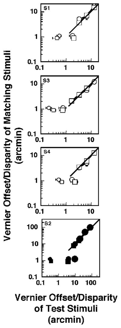
Threshold and matching data from the gap experiments for four observers. In each panel, the squares are data from the Vernier offset experiments and the circles are data from the stereo experiments. The error bars represent ±1 standard error. The unconnected square and circular symbols just below and above the y axis value of 1 in each panel represent the Vernier offset threshold and stereothreshold, respectively. The y axis value for the threshold data was selected arbitrarily. Small symbols correspond to thresholds for a 10′ interline gap (except S2’s gap=20′), medium-sized symbols correspond to thresholds for a 100′ gap (except S2’s gap=720′ and 240′ for Vernier offset and stereo-threshold experiments, respectively), and the large filled circle in the lower right panel corresponds to S2’s stereo threshold for a 540′ gap. The squares and circles joined by lines are data from suprathreshold Vernier offset and stereo experiments, respectively. The 1:1 diagonal line represents equal suprathreshold perception of the test and matching stimuli in the threshold unelevated and elevated conditions. The filled symbols for S2 denote that the gap of the matching stimuli in the Vernier offset and stereo suprathreshold experiments was 20′.

2. Stereoscopic Depth Experiments

To measure the stereothreshold, the relative disparity between the top and the bottom lines was manipulated using the stimulus configuration in Fig. 1(b). The observers judged whether the bottom line was in front of or behind the top line. For all observers except S2, the interline separations of the stereo targets were identical to those in the Vernier-threshold experiment. The interline separations used for S2 were 20, 240, and 540′, in order to produce an increased range of stereo thresholds. Relative disparity thresholds were computed from psychometric functions as described above and averaged across two to three replications per condition and observer.

To compare the perception of suprathreshold depth for stimuli with different interline gaps, the stimulus configuration in Fig. 1(b) was used for the test and matching stimuli. For all observers except S2, the interline separations in this experiment were identical to those used in the suprathreshold position-offset experiment above. After each trial, the observer indicated whether the interval with the test or matching stimulus contained the larger perceived magnitude of depth. In separate sessions, S2 matched perceived suprathreshold depth using test stimuli with interline gaps of 240 and 540′. For this observer, the interline gap for the matching stimulus was 20′.

B. Blur Condition

In these experiments, the elevation of position-offset and disparity thresholds was produced by introducing +2 D of dioptric blur. Dioptric blur was used because of its clinical relevance, but other forms of blur (e.g., Gaussian) could have been used instead. The same procedures that were used above in the threshold and suprathreshold gap conditions were used in these experiments, first to determine position-offset and disparity thresholds with and without +2 D of blur and subsequently to match the perceived suprathreshold position-offset and stereoscopic depth for these blurred targets.

1. Position-Offset Experiments

Vernier position-offset thresholds were measured with and without +2 D of binocular image blur in separate sessions. Dioptric blur was introduced by a pair of +2 D lenses mounted in a hand-held plastic frame (known clinically as “flippers”) that the observer held directly in front of his or her eyes. Some additional measurements were made for observer S3 using +4 D lenses in front of both eyes. The interline gap in the binocular stimulus [see Fig. 1(a)] was fixed at a value of 20′. Other aspects of the procedures and data analyses were identical to those described above for the gap-threshold position-offset experiment.

To match perceived suprathreshold position offset, the blurred test stimulus [see Fig. 1(a)] was viewed for 200 ms, 200 ms after the bright fixation cross disappeared. Blur was produced by viewing through a pair of +2 D lenses (also +4 D for observer S3) in front of the observer’s eyes. During the subsequent 2 s presentation of the fixation cross, the observer removed the lens flippers in order to view the unblurred matching stimulus for 200 ms. In this experiment, the interline gap for both the test and matching stimuli was always 20′. The data plotted in Fig. 3 for each observer represent the average of at least two replications per suprathreshold position-offset for both the leftward and rightward directions.

Fig. 3.

Threshold and matching data from the blur experiments for three observers. The unfilled symbols indicate that the test target was blurred by +2 D. Otherwise, the lines and symbols have the same meaning as in Fig. 2. The interline gap was 20′. For observer S3 a test target with 4 D blur also was used (filled symbols).

2. Stereoscopic Depth Experiments

Stereoscopic disparity thresholds were measured with and without +2 D of blur using the stimulus configuration shown in Fig. 1(b). The interline gap was 20′, and for all observers except S5 the duration of the disparity stimulus was 200 ms. For observer S5 the stimulus duration was increased to 500 ms, as this duration produced thresholds that were considerably less variable. Note that many studies have suggested that stereopsis is mediated by two separate systems: a transient and a sustained system, e.g. [14]. However, the integration times of both these systems are expected to be lower than 200 msec [15]. Thus, even if we were to use a disparity stimulus duration of 500 msec for subjects other than S5, we would expect the results of our experiments to change minimally.

The procedures used to match the perceived suprathreshold depth between a pair of blurred lines [Fig. 1(b)] were identical to those for suprathreshold position-offset above. As in the stereoscopic threshold experiment, the test and matching stimuli for observer S5 were presented for a duration of 500 ms.

C. Perceived Stimulus Distance

For a fixed magnitude of stereoscopic disparity, perceived depth increases approximately with the square of the distance at which the disparate targets are viewed [16]. This relationship between perceived depth and (veridical) information about the viewing distance leads to the phenomenon of stereoscopic depth constancy [17]. Similarly, the perceived size of a visual stimulus depends on the distance information [16]. We therefore assessed the influence of blur on the perceived distance of the stimuli for the three observers who participated in the threshold and suprathreshold blur experiments to determine whether perceived position-offset and stereoscopic depth were influenced systematically by possible blur-induced distortions of perceived distance information. Perceived distance was estimated with and without +2 D of binocular blur by comparing the blurred and unblurred line stimuli that were viewed in the haploscope to a subsequently viewed clear object in free space. Perceived distance matches were obtained in a dimly lit laboratory room by varying the physical distance of the unblurred comparison object.

3. RESULTS

A. Gap Condition

1. Vernier Position-Offset Thresholds

As shown by the horizontal separation between the unconnected squares in Fig. 2, an increase in the interline gap elevates the threshold for Vernier offset. The Vernier thresholds averaged across observers (excluding observer S2) for the smaller and larger interline gaps are 28.3±10.9 (SD) and 99.5±48.4″, respectively. The elevation of the Vernier offset threshold (the ratio of the threshold for the larger versus the smaller gap for each observer) averaged across observers S3, S4, and S1 is by a factor of 3.4±1.2 (SD). For observer S2, the Vernier thresholds are 20.7 and 219.2″ for the 20 and 720′ gaps, respectively, representing an elevation of 10.6 times. Because we define the threshold elevation as the ratio of the thresholds in the elevating and the nonelevating conditions, similar threshold elevations imply similar distances on logarithmic plots, such as those shown in Fig. 2.

2. Suprathreshold Position Offsets

Although the Vernier threshold was elevated by an average factor of ~3.5, matched suprathreshold position offsets are essentially the same for stimuli with small and large gaps (the connected unfilled squares in Fig. 2). Further, despite an approximately tenfold elevation of the Vernier thresholds for observer S2 (obtained by increasing the range of interline gaps; connected filled squares in Fig. 2), the relationship between the matched position offset for suprathreshold stimuli with smaller and larger gaps is the same as that found for the other three observers. A three-factor mixed model analysis was performed to compare the Vernier offsets of the suprathreshold stimuli in the threshold-elevated (larger interline gap) and threshold-unelevated conditions (smaller gap). All the analyses were performed using SAS 9.1, Cary, North Carolina. Recall that the perceived Vernier offsets resulting from the suprathreshold stimuli in the two conditions were equal.

The three factors in the model were condition (unelevated, elevated), offset direction (left, right), and level (a continuous variable corresponding to the log of the test stimulus offset). The dependent variable was the log of the Vernier offset in the matching stimulus. For the unelevated condition, dummy data were inserted in which the level and dependent variable were equal. This step was based on the assumption that matching perceived Vernier offset in a test stimulus to that in a matching stimulus, where both stimuli had smaller (and equal) gaps, would result in zero error. This analysis tests if the ratio of the Vernier offsets in the two test conditions differs significantly from unity. (The same analyses were used also in the other three suprathreshold experiments presented below.) We considered only the main-effect terms in the model, and the covariance structure was first-order autoregressive.

This analysis provided no evidence that the Vernier offsets in the threshold-elevating (larger gap; mean log offset=2.53±0.04 SE) condition were different from those in the unelevated condition (smaller gap; mean log offset=2.53±0.04 SE; F[1,3]<0.01, p=0.97). Because the previous analyses included dummy data, to determine if the offset direction was a significant factor in the raw experimental data we chose to run a second two-factor mixed model analysis (The parenthetical note above applies to this analysis also.) The two factors in the second analysis were offset direction (left, right) and level (a continuous variable corresponding to the log of the test stimulus offset). The dependent variable was still the log of the Vernier offset in the matching stimulus. Once again we considered only the main effect terms in the model, and the covariance structure was first-order autoregressive. There was no evidence that the perceived magnitude of Vernier offset depended on the direction of the offset (mean for left offsets=2.52±0.06 SE, mean for right offsets=2.54±0.06 SE; F[1,3]=2.62, p=0.2).

3. Stereothresholds

As shown by the horizontal separation of the unconnected circles in Fig. 2, an increase in the interline gap also elevates stereothresholds. The stereothresholds averaged across all observers (except S2) for the smaller (20′) and larger (100′) interline gaps are 24.8±10.7 and 85.5±35.1″, respectively. The elevation of stereothreshold averaged across all the observers (except S2) is 3.5±0.12 times. Stereothresholds for observer S2 are 18.9, 244.8, and 585.6″ for 20, 240, and 540′ gaps, respectively. The data for the two larger interline gaps correspond to threshold elevations of 12.9 and 31 times. In contrast to the results reported by Berry [9], increasing the gap size produces a greater elevation of the stereo than the Vernier-offset threshold in all of the observers except S1 (Vernier elevation=4.7,2.3,3.3; stereo elevation =3.4,3.6,3.4 for subjects S1, S3, S4). In fact, for observer S2, the elevation of the stereothreshold is larger than that of the Vernier-offset threshold even though the gap sizes used in the stereo experiment are substantially smaller (240 and 540′ in the stereo experiment versus 720′ in the Vernier offset experiment).

4. Suprathreshold Stereoscopic Depth

Despite elevation of stereothresholds by an average factor of 3.5 in three of the observers (all except S2), the matched suprathreshold disparities were essentially the same for stimuli with small and medium gaps (connected unfilled circles in Fig. 2). For subject S2 (connected filled circles in Fig. 2), approximately 13-and 31-fold elevations of the stereothresholds were obtained by increasing the interline gaps from 20′ to 240′ and 540′, respectively. Despite the substantially larger extent of threshold elevation for this subject, the relationship of matched position-offset between suprathreshold stimuli with small and larger gaps (Fig. 2, lower right panel with connected filled circles) was the same as that found for the other three observers. For the four observers, the ranges of matching disparities were 100–4800″ and 90–5771″ in the threshold-elevated and -unelevated conditions, respectively. A mixed-model analysis (similar to that discussed above for suprathreshold position-offsets) was performed to compare the disparities of the suprathreshold stimuli in the threshold-elevated condition (medium and larger gaps) to those of the suprathreshold stimuli in the threshold-unelevated condition (smaller gap). This analysis yielded no evidence that the disparities in the threshold-elevating condition (mean log disparity =2.7±0.05 SE) were different from those in the unelevated condition (mean log disparity=2.69±0.06 SE; F[1,3]=1.22, p=0.35). In addition, there was no evidence that the perception of stereoscopic depth depended on the direction of the disparity (mean log uncrossed disparity =2.7±0.09 SE, mean log crossed disparity=2.66±0.07 SE; F[1,3]=0.73, p=0.46).

B. Blur Condition

1. Vernier Position-Offset Thresholds

As shown by the horizontal separation of the unconnected, unfilled squares in Fig. 3, the introduction of +2 D of blur elevates the thresholds for Vernier position offset. The Vernier thresholds averaged across all observers for unblurred and blurred stimuli are 22.9±7.7″ (SD) and 75.2±13.9″, respectively. The elevation of Vernier threshold averaged across all observers is 3.4±0.8 times. Additional data for observer S3 (unconnected filled square) indicates that +4 D of blur elevates the Vernier position-offset threshold even further, by a factor of ~12 times above this observer’s threshold in the absence of blur.

2. Suprathreshold Position Offset

Despite elevation of Vernier threshold by a factor of approximately 3.5, the matched suprathreshold position-offsets are essentially the same for unblurred and +2 D blurred (connected unfilled squares in Fig. 3). A mixed-model analysis (see note above) provided no evidence that the perception of position-offset in the threshold-elevating condition (+2 D blur, mean log offset=2.55±0.03 SE) is different from that in the unelevated condition (no blur, mean log offset=2.52±0.04 SE; F[1,2]=3.79, p=0.19). Further, there is no evidence that the perception of Vernier offsets depends on the direction of the offset (mean log left offset=2.54±0.06 SE, mean log right offset =2.49±0.0 SE; F[1,2]=4.84, p=0.16).

When viewing through +4 D of blur, observer S3 underestimated the magnitude of suprathreshold position-offsets up to approximately three times his elevated position-offset threshold (connected filled squares in the right panel of Fig. 3). However, for larger magnitudes of suprathreshold position-offset (i.e., 4 and 6 times the Vernier offset threshold with +4 D of blur), the perceived magnitudes with and without 4 D of blur are essentially identical.

3. Stereothresholds

As shown by the horizontal separation of the unconnected circles in Fig. 3, blur elevates the stereothresholds. Averaged across all observers, the stereothresholds for the unblurred and +2 D blurred stimuli are 31.8″ ±11.9″ (SD) and 247.7″ ±44.4″, respectively. The elevation of stereo-threshold averaged across all observers is by a factor of 8.4±2.4. In all observers, the elevation of stereothreshold produced by +2 D of blur is larger than the elevation of the Vernier offset threshold (Vernier elevation =3.1,4.4,2.9; stereo elevation=6.7,11.1,7.3 for subjects S2, S3, S5).

4. Suprathreshold Stereoscopic Depth

The perception of depth produced by suprathreshold disparities was reduced substantially for blurred compared to unblurred targets (connected circles in Fig. 3). For the three observers who were tested, the ranges of matching disparities were 300–1149 and 52–902″ in the blurred and unblurred conditions, respectively. Moreover, for each observer, the reduction of perceived depth for the +2 D blurred targets was consistent and represented an approximately constant proportion of the suprathreshold disparity magnitude, as shown by the approximately constant logarithmic distance of the connected circles below the 1:1 line in Fig. 3. A mixed-model analysis (see note above) indicated that the disparities in the blurred condition (mean log disparity=2.75±0.03 SE) were significantly higher than those in the unblurred condition (mean log disparity=2.43±0.05 SE; F[1,2]=147.8, p =0.007). However, the perception of stereoscopic depth did not depend on the direction of the disparity (mean log uncrossed disparity=2.43±0.07 SE, mean log crossed disparity=2.44±0.07 SE; F[1,2]=0.28, p=0.65).

5. Perceived Distance

Because the perceived magnitude of stereoscopic depth depends on information about the viewing distance [16,17], the erroneous perception of suprathreshold depth when the targets are blurred might be attributable to a change in their perceived distance. To examine this possibility, we compared the ratio of the squared perceived stimulus distance with and without +2 D of blur to the ratio of stereoscopic disparities that produced the same perceived depth without and with +2 D of blur. The logic behind this comparison is that stereoscopic depth constancy predicts that the perceived depth between a pair of targets with a fixed suprathreshold disparity should vary directly with the square of the stimulus distance:

$$\mathit{Perceived}\mathit{Depth}=k(\mathit{Disparity})(\mathit{Viewing}{\mathit{Distance}}^2),$$ (1)

where k is a constant. If we assume that the same information is responsible for perceived distance and for scaling perceived depth [18], then the ratio of disparities that produce equal magnitudes of perceived depth without and with target blur should be equal to the ratio of the squared perceived distances with and without blur. These ratios are plotted against each other and shown for each of the three observers as the circles in Fig. 4. Ratios of the matched disparities less than unity imply that the amount of perceived depth is reduced for a blurred compared with an unblurred target with the same disparity. Although all of the ratios are less than one, a comparison of the circles with the diagonal line in Fig. 4 indicated that the decrease in the squared perceived distance with +2 D of blur was unrelated to the decrease in perceived stereoscopic depth. For observers S2 and S3, +2 D of blur did not decrease the perceived target distance enough to account for the blur-induced reduction of perceived stereoscopic depth. In contrast, observer S5 showed a greater reduction of the squared perceived distance than of perceived depth with +2 D of blur.

Fig. 4.

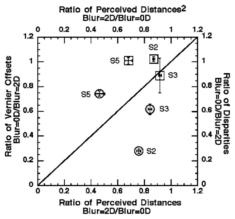
Relationship between blur-induced changes in perceived target distance and perceived position-offset (squares) or stereoscopic depth (circles). The top x axis and the right-hand y axis compare the ratio of the squared perceived distances for blurred versus unblurred targets to the ratio of disparities for unblurred matching and blurred test stimuli, averaged for all of the suprathreshold disparities in Fig. 3. The bottom x axis and left-hand y axis compare the ratio of perceived distances for blurred versus unblurred stimuli to the ratio of the Vernier position offsets for unblurred matching and blurred test stimuli, averaged for all the suprathreshold Vernier offsets in Fig. 3. Each symbol represents the data for one observer, with x and y error bars equal to ±1 SE. The diagonal line indicates that blur-induced changes in perceived stereoscopic depth or relative position offset can be accounted for by blur-induced changes in perceived distance.

Analogous to stereoscopic depth constancy, size constancy predicts that the magnitude of the perceived position-offset produced by a specific angular separation between the line targets should vary directly in proportion to the perceived distance [18–20]. Consequently, for equal perceived suprathreshold Vernier position offsets, we also compared the ratio of perceived stimulus distance with and without +2 D blur to the ratio of the Vernier stimulus offset without and with blur (Fig. 4, squares). In Fig. 4, ratios of matched position offset less than unity indicated that the perceived Vernier offset is less for a blurred compared with an unblurred target with the same physical offset. A comparison of the squares with the diagonal line in Fig. 4 indicated that, for observers S2 and S5, the introduction of +2 D of blur produced a greater decrease of perceived target distance than of the perceived Vernier offset. For observer S3, the blur-induced decrease in perceived distance and position offset was similar. Although size constancy can account for the slight reduction of perceived Vernier position offset in the blurred compared with unblurred condition in observer S3, it should be noted that stereoscopic depth constancy does not explain the blur-induced reduction of perceived stereoscopic depth in that observer.

4. DISCUSSION

A. Prevalence of Suprathreshold Normalization and Its Dependence on Threshold Elevating Condition

We measured threshold and suprathreshold perception for two distinct visual functions, namely, relative position perception and stereoscopic depth perception. For both functions, we used the same binocular stimulus and only the conjugacy between the position offsets in the two eyes’ images was different (conjugate for relative position perception and disconjugate for stereoscopic depth perception). For each visual function, suprathreshold perception was measured in two threshold-elevating conditions: (1) an increase in interline separation within the stimulus and (2) dioptric blur of the retinal image. For the range of parameters we tested, both the suprathreshold perception of relative position and stereoscopic depth are essentially unaffected by the threshold elevation caused by increasing the interline gap in the stimulus. This indicates that the normalization of suprathreshold perception applies to visual functions other than contrast perception. The suprathreshold perception of relative position offset was also normalized when the threshold elevation was caused by blur of the retinal image. However, the suprathreshold perception of stereoscopic depth was not normalized when the threshold elevation was caused by blur. These results suggest that the normalization of suprathreshold perception depends on the visual function under consideration and how the threshold is elevated. We discuss these data from descriptive and mechanistic points of view in Subsections 4.B and 4.C below.

B. Descriptive Models of Suprathreshold Perception

One of the simplest descriptive models for perception is an affine model. When a suprathreshold stimulus s₀, presented under a condition for which the threshold is Th₀, is perceived to match another suprathreshold stimulus s_e, presented under a condition for which the threshold is Th_e, the following equation can be derived from the affine model [Eq. (A3) in Appendix A]:

$$k_e(s_e-{Th}_e)=k_0(s_0-{Th}_0).$$ (2)

In Eq. (2) k₀ and k_e are proportionality constants for the conditions that yield thresholds Th₀ and Th_e, respectively. Note that we assume implicitly that the perceived magnitudes of threshold stimuli in the two conditions are equal, i.e., P_Th0 = P_The. When k_e= k₀, Eq. (2) reduces to

$$s_e-{Th}_e=s_0-{Th}_0.$$ (3)

Equation (3) describes the Kulikowski model, which states that equal perception occurs in the two conditions when the stimuli are equal amounts above their corresponding thresholds. In Fig. 5(a) we illustrate the predictions of Kulikowski’s model of suprathreshold perception for two conditions in which the thresholds are Th₀ and Th_e. Kulikowski [8] proposed this model to relate suprathreshold contrast perception to contrast thresholds for various spatial frequencies of the stimulus. Other models of suprathreshold contrast perception are functionally similar [3,7]. When the stimulus and response magnitudes are plotted on a log–log plot, the graphical representation of Kulikowski’s model is as shown in Fig. 5(b).

Fig. 5.

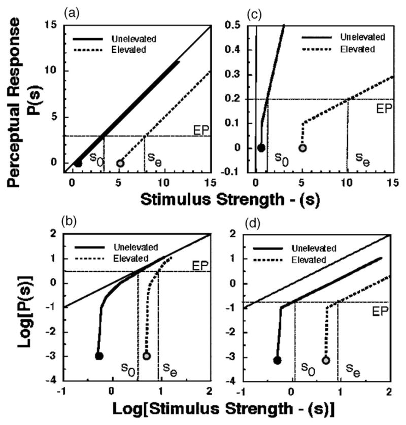
Relationship between the threshold and the perception of suprathreshold stimuli as predicted by Kulikowski’s [(a) and (b)] and by proportional models [(c) and (d)] of suprathreshold perception. (a) and (c) plot stimulus strength s versus the perceptual response P(s) on linear x and y axes. (b) and (d) replot the same relationships on logarithmic x and y axes. In each plot, the thick black line shows the relationship between stimuli and perceptual responses for stimulus levels above the unelevated threshold Th₀ (black circle). In a threshold-elevating condition, the threshold increases to Th_e (gray circle) and perceptual responses to stimuli greater than Th_e are defined by the thick dotted line. In the model shown in (a) and (b), the perceptual responses EP in the normal and threshold-elevating conditions match when the suprathreshold stimuli in the corresponding conditions s₀ and s_e differ by the amount equal to the difference between the thresholds (Th_e − Th₀). In the model shown in (c) and (d), the perceptual responses EP in the normal and threshold-elevating conditions match when the suprathreshold stimuli in the corresponding conditions s₀ and s_e have a ratio equal to the ratio of the thresholds Th_e/Th₀. Note that the proportional model’s prediction in the logarithmic coordinate system is equivalent to the Kulikowski model’s prediction in a linear coordinate system.

The equation that describes suprathreshold perceptual equality under conditions that have different thresholds, as derived either from Stevens’s power law or the Weber–Fechner law of perception [Eqs. (A7) and (A10) in Appendix A], is

$$k_e(log{s}_e-log{Th}_e)=k_0(log{s}_0-log{Th}_0).$$ (4)

For the above equation we again assume that the perceived strength of threshold stimuli in the two conditions is equal, i.e., P_Th0 = P_The. When k_e= k₀, Eq. (4) reduces to

$$log{s}_e-log{Th}_e=log{s}_0-log{Th}_0.$$ (5)

Equation (5), termed the proportional model, states that suprathreshold stimuli should be perceived as equal when they are equal multiples of their respective threshold values. Figures 5(c) and 5(d) illustrate the predictions of the proportional model for conditions in which the thresholds are Th₀ and Th_e. To a first approximation, the proportional model provides an adequate description of perceived suprathreshold brightness—if sensitivity is expressed on a logarithmic axis—as the photopic spectral luminosity function determined by suprathreshold brightness matching approximately parallels the spectral sensitivity function determined from foveal light detection thresholds [21,22].

To determine the extent to which the data from our experiments are consistent with the predictions of the Kulikowski and proportional models, we performed regression analyses using our entire data set. Specifically, we determined how well our data fit the relationship between (s_e− Th_e) and (s₀ − Th₀) and between [log(s_e) − log(Th_e)] and [log(s₀) − log(Th₀)], and how close the slopes of the fitted lines are to the predicted value of unity. The results of these regression analyses are shown in Figs. 6 and 7. Note that (s_e − Th_e) and [log(s_e) − log(Th_e)] were assigned arbitrarily as the dependent variables. The summary statistics for the regression analyses are given in Table 1.

Fig. 6.

(Color online) Evaluation of the Kulikowski (top row) and proportional models (bottom row) for suprathreshold perception, using data pooled across observers and conditions in the gap (left) and blur (right) position-offset experiments. The x axis in each panel represents the difference between the suprathreshold position offset and the threshold Vernier offset (linear in the top panels and log transformed in the bottom panels) when the Vernier threshold was not elevated. The y axis represents the difference between the suprathreshold position offset and the elevated Vernier threshold in threshold-elevating conditions. Filled circles specify position offsets in the threshold-unelevated and elevated conditions that perceptually match. Solid lines are fit to the plotted data, with the y intercept constrained to be zero. In each panel, the prediction of the Kulikowski or the proportional model is shown by a dotted line.

Fig. 7.

(Color online) Evaluation of the Kulikowski (top row) and proportional models (bottom row) for suprathreshold perception using the data from the stereoscopic depth experiments. The x axis in each panel represents the difference between the suprathreshold disparity and the stereothreshold (linear in the top panels, log transformed in the bottom panels) when the stereothreshold was not elevated. The y axis represents the difference between the suprathreshold disparity and the elevated stereothreshold in threshold-elevating conditions. Other conventions are as in Fig. 6.

Table 1.

Summary of Regression Analysis to Test Kulikowski and Proportional Models^a

Regression Analysis		Conditions
		Gap			Blur
Function	Model	Slope	Adj R2	p	Slope	Adj R2	p
Vernier	Kulikowski	0.83	0.98	<0.001	0.85	0.98	<0.001
	Proportional	0.52	0.90	<0.001	0.45	0.91	<0.001
Stereo	Kulikowski	0.7	0.99	<0.001	1.12	0.91	0.3
	Proportional	0.4	0.83	<0.001	0.38	0.91	<0.001

^aThe p values indicate whether the fitted slope differs significantly from unity.

As expected, all the regression lines in Figs. 6 and 7 have slopes that differ significantly from zero (highest p value=0.001). In all cases, better fits were obtained for regression lines without intercepts than with intercepts, as determined by comparing the corresponding adjusted R² statistic [Adj·R²=1− ((1 − R²)(n − 1)/(n − k − 1)), where R², n, and k are the coefficient of determination, number of observations, and number of model parameters, respectively]. Because the adjusted R² takes into account the cost associated with increasing the number of parameters in a model, it is better suited than the unadjusted values of R² for comparing models with unequal numbers of parameters. When the y intercept was not constrained to be zero, the fitted intercept was found to be significantly different from zero in only one condition (Fig. 6, bottom left panel; p=0.01). Here, the nonzero offset can be interpreted to mean that the perceived Vernier position offset produced by threshold stimuli with the small and large gaps in our experiments do not match, i.e., P_Th0 ≠ P_The (see Eqs. (A7) and (A10) in Appendix A). In the following we will discuss only the results of the regression models without the y intercept.

The adjusted R² values shown in Table 1 indicate that both regression models account reasonably well for the variance of the data in our Vernier offset and stereo experiments. Overall better fits (i.e., higher adjusted R² values, t[3]=2.4, p<0.1) were obtained using the Kulikowski [Eq. (3), mean=0.97, SD=0.04] than the proportional [Eq. (5), mean=0.89, SD=0.04] model. The p values in Table 1 indicate that the slopes of the regression lines are significantly different from unity for virtually all of the conditions shown in Figs. 6 and 7, except for the +2 D blur condition in the top right panel of Fig. 7. Because both the Kulikowski and the proportional model require the slope of the fitted regression line to be unity, this outcome suggests that neither model can adequately account for our data. However, the overall slopes for the Kulikowski model (mean=0.88, SD=0.18) are significantly greater (t[3]=4.2, p<0.05) than those for the proportional model (mean=0.44, SD=0.06). The slopes of the regression lines in Figs. 6 and 7 specify the ratio of k_e to k₀ in each model for each of the experimental conditions. In the context of the Kulikowski and proportional models, a deviation of the fitted regression line from a slope of unity implies that k_e and k₀ are different, which means that the threshold-elevating condition produces a change in the underlying sensory-perception transducer function (specifically, a gain change in the affine and Weber–Fechner models and a change of exponent in the Stevens model).

C. Mechanisms Underlying Normalization of Suprathreshold Perception

1. Relative Position Perception

Under the conditions of our experiments, the perceived absolute position of a sufficiently visible stimulus is thought to be determined by the location of the responding neurons on a topographical retinal map in the visual cortex [23,24]. Each neuron in this topographical map is presumed to have a position label, called its local sign, so that regardless of its activity level the neuron always signals the same retinal position. Because even the tiniest target stimulates more than a single retinal photoreceptor, it is likely that multiple position labels are active for any single target, allowing a population position code to be formed [25,26]. Consequently, the perception of a target’s absolute position may be determined by a weighted combination (e.g., centroid) of the position labels of the active neurons. To determine the difference in position between two targets, the population activity generated by each target is compared prior to a perceptual decision [27]. In this framework for relative position computation, the threshold can be attributed to (1) noise in the position label of each neuron in the map, (2) noise in the activity of each neuron in the map, and (3) noise in the mechanism that combines or compares the two population position codes from the map (a collator mechanism). The neural basis for noise in the position label is not clear, but random fluctuations in spontaneous and stimulus-induced firing rates in the presynaptic circuitry, perhaps due to random failures at the synapses, are reasonable possibilities. The noise in the collator mechanism may be due to random fluctuations in the orientation tuning of the neurons that constitute the collator mechanism. There is evidence that a orientated mask presented simultaneously with a Vernier stimulus affects relative position thresholds [28–30] even for large interline gaps [30], which Mussap and Levi [31] attributed to the influence of the mask on the collator mechanism. Because of these noise sources, the relative position signal that is used to make perceptual decisions can be assumed to be stochastic. As the spatial gap between two Vernier targets increases, the position noise in component (1) should increase because at least one set of the neurons that forms the population position code will represent more peripheral retina and use larger receptive fields. Noise in component (3) should also increase as the interline gap increases if larger receptive fields are used to combine the individual population position codes [31,32].

The relative position computation model with the above-mentioned noise sources is described mathematically in Appendix B. This model was simulated and its parameters were determined using targets with 10′ and 100′ gaps and the corresponding empirically measured Vernier thresholds of ~30″ and 210″. As can be seen from Table 2, the elevation of threshold for 100′ gap targets relative to 10′ gap targets can be attributed to (a) a decrease in spatial resolution of the topographical map by a factor of 2, (b) a corresponding increase in position-label noise by a factor of 2, and (c) an increase in noise in the collator mechanism by a factor of 3.2. Using the same parameters, the model determined the Vernier offsets in the threshold-unelevated condition (gap=10′) that matched the suprathreshold Vernier offsets in the threshold-elevated condition (gap=100′). As can be seen from Table 3, in total agreement with our empirical results, the model predicts perfect normalization of suprathreshold Vernier offsets presented in the threshold-elevated condition.

Table 2.

Parameters of the Relative Position Computation Model (Gap Experiment)

Parameter	Gap=10 min	Gap=100 min
r1, r2 (arcsec)	15	30
g1, g2	1	1
η1 for all neurons, η2 for all neurons	0.5	0.5
σ1, σ2	8	4
ε1 for all neurons, ε2 for all neurons	0.1	0.1
λ1, λ2	16	8
φ (arcsec)	37.5	120

Table 3.

Results of Simulating the Suprathreshold Vernier Gap Experiment

Vernier Offset in a 100′ Gap Target (arcsec)	Matched Vernier Offset in a 10′ Gap Target (arcsec)
240	238
480	478
720	717
960	958

The introduction of dioptric blur removes high spatial frequencies from the target’s image and reduces the peak of the retinal luminance distribution of each line. In terms of each neuron in the topographical map, the reduction of high spatial frequencies would result in inactivation of neurons with smaller receptive fields in the presynaptic circuitry. This would cause an increase in the position-label noise for each neuron in the map. We simulated the model again and determined the parameters using unblurred and blurred (2 D) targets and the corresponding Vernier offset thresholds of ~30″ and 90″. As seen in Table 4, the elevation of Vernier threshold of blurred relative to unblurred targets can be attributed to (a) an 80% decrease in peak activity in the map, (b) an increase in the dispersion of the neural activity by a factor of 2, (c) a corresponding increase in the set of neurons contributing to the absolute position computation by a factor of 2, and (d) an increase in the position-label noise by a factor of 32. In agreement with empirical data, simulations of suprathreshold Vernier offsets for blurred and unblurred targets once again indicate perfect normalization (data not shown). In summary, the perception of suprathreshold position offset is largely veridical when the threshold is elevated by an increase in the interline gap or dioptric blur. Veridical perception in these conditions can be attributed to the encoding of relative position within topographical maps.

Table 4.

Parameters of the Relative Position Computation Model (Blur Experiments)

Parameter	Blur=0	Blur=2 D
r1, r2 (arcsec)	15	15
g1, g2	1	1/8
η1 for all neurons, η2 for all neurons	0.5	16
σ1, σ2	8	16
ε1 for all neurons, ε2 for all neurons	0.1	0.1
λ1, λ2	16	32
φ (arcsec)	37.5	37.5

2. Stereoscopic Depth Perception

Instead of a map of retinal-position labels, one can hypothesize that the processing of stereoscopic depth starts with a map of absolute disparity detectors [24,33–36]. Analogous to position, each target’s absolute disparity is encoded by a population of disparity-labeled neurons [37–42]. The relative disparity between two targets can be computed by combining or comparing the population disparity codes of the two separate targets. Consequently, the neural mechanisms for computing relative position offset and relative disparity from absolute positions and absolute disparities, respectively, have identical architectures. For the threshold-elevating conditions of line separation and dioptric blur, one might therefore expect that the perception of suprathreshold disparity would behave similarly to suprathreshold position offset. However, as seen in Fig. 7 (also see the slopes of the regression lines in Table 1), the perception of suprathreshold stereoscopic depth is affected differently by the threshold-elevating conditions of increased gap and dioptric blur. Like the perception of suprathreshold position offset, the computation of suprathreshold stereoscopic depth is robust to changes in the interstimulus gap. However, unlike the perception of suprathreshold relative position, perceived stereoscopic depth is not robust to the combination of the decrease in the peak retinal luminance and the loss of high spatial frequencies that results from blur. This outcome indicates that one or more additional factors that do not have a strong role in the perception of relative position exert a substantial influence on the perception of stereoscopic depth.

Because information about absolute distance is required to perceptually scale stereoscopic image disparity [16], one possibility is that the misperception of the depth between blurred targets is attributable to a systematic misregistration of the blurred targets’ distance. However, the data from our auxiliary experiment indicate that the nonveridical perception of stereoscopic depth can not be accounted for by errors in the perceived distance of blurred targets. An alternative possibility is that an error occurs in the computation of relative disparity for these targets. Why should the computation of suprathreshold relative disparities be erroneous when the targets are blurred?

One possibility is that the representation of absolute disparities on a topographical disparity map is weighted by a function that reduces the contribution of disparities that are farther from the horopter. One line of evidence for such a weighting function comes from previous experiments that showed stereo matches in the fixation plane are preferred over matches that result in large disparities [43,44]. Additional evidence for the weighting of disparity signals comes from a study by Stevenson et al. [45], who showed a monotonic increase in interocular correlation thresholds with an increase in the distance of the binocular stimulus from the horopter. Horopter-dependent disparity weighting was implemented in a model of disparity processing by Prince and Eagle [46], who successfully explained a wide range of data on stereopsis for first- and second-order stimuli. Figure 8 illustrates how this idea applies to our data.

Fig. 8.

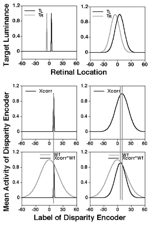
Illustration of the effect of stimulus blur and readout weighting on disparity representation. The top row illustrates the retinal activity profiles generated by one object of a binocular stimulus that is composed of two objects. The second object (not shown) is assumed to lie on the horopter with zero disparity. Activity profiles in the two eyes are represented as two Gaussian functions (curves T_L and T_R) displaced from the retinal zero location in opposite directions. The difference between the peaks of the two Gaussian functions represents the absolute stimulus disparity (here, 10′). The middle row shows the absolute disparity representation obtained by cross-correlating the retinal activity profiles in the two eyes in the top row. The gray Gaussian curves (W_f :SD=20′) in the bottom row depict a hypothetical weighted readout function for disparity, and the black curves represent the weighted disparity representation computed by multiplying the absolute disparity representation in the middle row by the weighted readout function. The left and right columns show the normalized retinal activation and the corresponding disparity representations for an unblurred (Gaussian SD=0.5′) and a blurred stimulus (Gaussian SD=10′), respectively. The long vertical dotted lines that span the second and third rows illustrate the relative alignment between the peaks of the disparity representation and the weighted disparity representation.

The top row of Fig. 8 illustrates the retinal activity pattern generated by one of the two objects in our binocular stimulus. The activity patterns generated by this object in the left and the right eyes are superimposed in the same plot. The second (comparison) object in the binocular stimulus is assumed to have zero absolute disparity, but, to maintain clarity, its retinal representations are omitted from the figure. Because the comparison object has zero disparity, the absolute disparity of the object that is shown in the figure is equal to the relative disparity between the two objects. The normalized luminance of each eye’s image is described by Gaussian functions (black and gray lines) that represent an unblurred object in the top left panel and a blurred object in the top right panel. Note that within each panel in the top row, the separation between the two Gaussian functions represents the absolute disparity of the object.

For the purpose of illustration, we used the output of a cross-correlation operation to represent the distributed absolute disparity code, as illustrated in the two panels in the middle row of Fig. 8. The disparity representation in each panel of the middle row is then multiplied by a weighted readout function (gray Gaussian curves in the bottom panels) and the resulting weighted disparity representations are shown as the black curves in the bottom row. For the unblurred stimulus, the location of the disparity representation (i.e., the disparity label with peak activity) is essentially unaffected by the weighted readout (indicated by the dotted vertical line that spans the middle and bottom left panels). On the other hand, both the peak and the centroid of the weighted disparity representation of the blurred stimulus are shifted toward zero disparity when compared to the unweighted disparity representation. The direction of this shift is consistent with our data that show a reduction of perceived depth in the presence of dioptric blur. The application of a weighted readout does not change the location of the disparity representation of the comparison object with zero absolute disparity because both the weighting function and the disparity representation have even symmetry with respect to zero disparity.

Figure 9 shows the results of simulating the weighted disparity computations for various disparity values and standard deviations (SDs) of the weighted readout function. As expected, Fig. 9 shows that readout weighting has no effect on the computed disparity of an unblurred stimulus. On the other hand, readout weighting has a substantial effect on the computed disparity of a blurred stimulus. As the SD of the weighting function increases (i.e., as the weighting function approaches a more rectangular distribution for the range of disparities considered here), the accuracy of the model’s response increases. The model’s responses for various suprathreshold disparities are qualitatively very similar to the empirical data shown as the unfilled circles in Fig. 3. Quantitative differences between the data of the three observers in Fig. 3 can be attributed to differences in the observer’s pupil sizes (which influences the magnitude of the retinal blur) and/or to differences in the SDs of their disparity weighting functions.

Fig. 9.

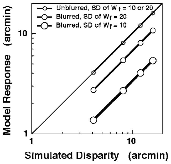
Simulation results for the weighted-disparity-computation model. The x axis represents the absolute disparity of an off-horoptoral binocular stimulus object. (The reference object is assumed to be on the horopter.) For each value of stimulus disparity on the x axis, the y axis represents the centroid of the weighted disparity representation obtained using a Gaussian weighting function W_f with its peak on the horopter as described in Fig. 8. Simulation results using two different weighting functions are shown for blurred (medium and large circles connected by slightly thick and thicker lines, respectively) and unblurred stimuli (small circles and thin connecting line). The standard deviation SD of the Gaussian retinal activity profile for the blurred stimulus was 10′. The thin diagonal line indicates veridical model responses.

It is worth recalling that dioptric blur does not have a comparable effect on the perception of suprathreshold relative position, which implies that a similar weighting of signals is not performed when readout occurs from the neural topographic position map. This differential treatment of disparity and position signals makes sense because, in the absence of a reference analogous to the horopter, there is no reason to weigh visual directions in the same way as disparity information.

The reduction of perceived depth for blurred targets may suggest a constraint for the coarse-to-fine model of stereopsis, which stipulates that large disparities are processed by low-spatial-frequency channels and small disparities are processed by high-spatial-frequency channels within the disparity map [47]. As mentioned above, one consequence of introducing dioptric blur is to reduce the luminance modulation of the high spatial frequencies in the stimulus. Specifically, if a pupil size of 4 mm is assumed, then +2 D of blur attenuates all spatial frequencies above approximately 2.5 cpd by at least 80%. Consequently, when a broad band target is blurred, the stereo threshold expressed in units of visual angle increases (compared with an unblurred stimulus) because the blurred target activates only disparity mechanisms tuned to low spatial frequency (coarse channels). If no interaction between coarse and fine disparity channels is assumed, then the loss of high spatial frequencies from the stimulus should not affect the encoding of suprathreshold disparities by the coarse channels and, hence, should not affect the perception of suprathreshold depth. For the coarse-to-fine model to account qualitatively for the reduction of perceived suprathreshold depth in blurred stimuli, some form of disinhibitory interaction from the fine channels onto the coarse channels would be necessary.

The reduction of perceived depth in the presence of 2 D of dioptric blur is consistent with the results of Schor and coworkers [6,48], who reported that the perception of suprathreshold stereoscopic depth is nonveridical for narrowband targets with spatial frequencies lower than approximately 2.5 cpd. Despite similar retinal stimulation (Fig. 1), the differential effect of dioptric blur on the suprathreshold perception of retinal position and stereoscopic depth provides additional support for the view that stereoscopic depth perception and relative position perception are mediated by separate neural mechanisms [9–11,49].

5. CONCLUSIONS

In summary, normalization of suprathreshold perception occurs for visual functions other than contrast perception. However, the perception of suprathreshold stimuli under conditions that elevate the visual threshold depends on the visual function and the threshold-elevating condition. For the conditions that we investigated in these experiments, the perception of position offset and stereoscopic depth cannot be completely accounted for either by Kulikowski’s or by proportional models of suprathreshold perception. We interpret our data within a neural framework of topographical encoding and readout mechanisms. This analysis assumes that absolute position and disparity signals are represented as population codes, and that both the codes and the mechanisms that read them out are susceptible to stochastic noise. We show that such an unbiased map-based encoding and readout scheme inherently has the property that changes in the mean and variance of the extracted signals are disassociated, resulting automatically in normalization. We suggest that the absence of normalization for the perception of depth in blurred stereoscopic targets reflects a coupling between changes in the mean and the variance of the stochastic mapping or readout processes, either because of signal weighting during readout of the relative disparity code or because of interactions between different spatial-frequency mechanisms that populate the disparity encoding map.

APPENDIX A: DESCRIPTIVE MODELS OF PERCEPTION

1. Affine Model of Perception

In this model, the perceived strength of the stimulus is related to the strength of the stimulus as in

$$P=ks+c,$$ (A1)

where P, s, k, and c are the perceived strength of the stimulus, the strength of the stimulus, a proportionality constant, and a constant bias, respectively. Perception in most cases occurs only when the strength of the stimulus is greater than a certain minimum value. Equation (A1) for this threshold condition is then given by

$$P_{Th}=k{s}_T+c,$$ (A2)

where P_Th and s_T are the perceived strength of the stimulus at threshold and the minimum strength of the stimulus needed for reliable perception, respectively. Substituting for c in Eq. (A1) we get

$$P=k(s-s_T)+P_{Th}.$$ (A3)

2. Stevens’s Model of Perception

In this model, the perceived strength of the stimulus is nonlinearly related to the strength of the stimulus. Mathematically, it is given by

$$P={cs}^k,$$ (A4)

where P, s, k, and c are the perceived strength of the stimulus, the strength of the stimulus, the power constant, and the gain, respectively. Transforming Eq. (A4) to the logarithmic coordinate system we get

$$logP=logc+\mathit{k}logs.$$ (A5)

At the threshold of perception,

$$log{P}_{Th}=logc+klog{s}_T.$$ (A6)

Substituting for log c in Eq. (A5) we get

$$logP=k(logs-log{s}_T)+log{P}_{Th}.$$ (A7)

Note that Eq. (A7) is also a linear equation but in a logarithmic coordinate system.

3. Weber–Fechner Model of Perception

In this model, the perceived strength of the stimulus is also nonlinearly related to the strength of the stimulus. Mathematically, it is given by

$$P=\mathit{k}logs+c,$$ (A8)

where P, s, k, and c are the perceived strength of the stimulus, the strength of the stimulus, the gain, and the offset, respectively. At the threshold of perception

$$P_{Th}=c+klog{s}_T.$$ (A9)

Substituting for c in Eq. (A8) we get

$$P=k(logs-log{s}_T)+P_{Th}.$$ (A10)

Note that Eq. (A10) is also a linear equation but in a semilogarithmic coordinate system. Further, note that the stimulus terms on the right-hand side of Eqs. (A7) and (A10) are identical.

APPENDIX B: MODEL OF RELATIVE POSITION PERCEPTION

Relative position computations in a topographical map

Consider two identical one-dimensional arrays or maps (M1 and M2) of cortical neurons. Let each array represent a contiguous retinal space of 4 deg in the horizontal meridian (2 deg nasal and 2 deg temporal). All neurons in arrays M1 and M2 represent the same retinal offset from a horizontal line (vertical offset) through the fovea in the upper and lower vertical meridians, respectively. To mimic the equal vertical distance of each line from the primary horizontal meridian in our experiments, the retinal vertical offsets represented by M1 and M2 are equal. Because of the cortical magnification factor, the horizontal spatial resolution of each array decreases with the magnitude of the vertical offset it represents. Each neuron in the array encodes an absolute horizontal position in retinal space, also known as position labels, which vary according to the horizontal spatial resolution. Mathematically

$$P_{ai}=i{r}_a-2+{\psi }_p,$$ (B1)

where P_ai denotes the position label of the ith neuron in array Ma (a is 1 or 2), r_a represents the resolution of the array Ma in units of visual angle, and ψ_p represents the noise sampled from a uniform distribution in the interval from −η_ai to η_ai units of visual angle. We define the neuron in the middle of the array to represent zero horizontal position. Let the top line of the Vernier target produce a Gaussian activation pattern in the array M1 centered at the neuron encoding zero horizontal position. Let the bottom line of the Vernier target produce a Gaussian pattern in the array M2 centered on the neuron encoding the desired Vernier offset. Mathematically

$$x_{ai}=g_{a}exp\left[-\frac{(i-n_{ac})}{2{\sigma }_a^2}\right]+{\psi }_x,$$ (B2)

where x_ai is the activation of the ith neuron, g_a is the peak activation, σ_a is the standard deviation, ψ_x is the noise sampled from a uniform distribution in an interval from 0 to ε_ai, and n_ac is the neuron with peak activity in the array Ma.

For the top line of the Vernier target n_ac=round(2/r_a), and for the bottom line of the Vernier target n_ac =round((2+V)/r_a), where V is the desired Vernier offset in deg. The absolute positions of the top T_top and bottom T_bottom lines in M1 and M2 are derived from the centroid of the activation pattern as given by

$$T_{\text{top}}=\frac{{\displaystyle \sum _{i=1}^{\text{round}(4/r_1)}}{P}_{1i}{f}_1(x_{1i})}{{\displaystyle \sum _{i=1}^{\text{round}(4/r_1)}}{f}_1(x_{1i})},$$ (B3)

$$T_{\text{bottom}}=\frac{{\displaystyle \sum _{i=1}^{\text{round}(4/r_2)}}{P}_{2i}{f}_2(x_{2i})}{{\displaystyle \sum _{i=1}^{\text{round}(4/r_2)}}{f}_2(x_{2i})},$$ (B4)

where

$$f_a(x)=\{\begin{array}{ll}x,\hfill & \text{if}{n}_{ac}-{\lambda }_a\le x\le n_{ac}+{\lambda }_a\hfill \\ 0,\hfill & \text{otherwise}\hfill \end{array}.$$ (B5)

In Eq. (B5), λ_a defines the neurons of the array around n_ac that contribute to the computation of the absolute positions of the lines.

Next, a collator mechanism compares the absolute positions of the top and bottom lines to yield a relative position signal RP as indicated by

$$RP=r_1{T}_{\text{top}}-r_2{T}_{\text{bottom}}+{\psi }_{rp},$$ (B6)

where ψ_rp is the noise sampled from a uniform distribution in a interval from −φ to φ units of visual angle. Finally, depending on the sign of RP, a perceptual decision D is generated as

$$D=\{\begin{array}{ll}\text{left}\text{if}\hfill & RP<0\hfill \\ \text{right}\text{if}\hfill & RP>0\hfill \\ \text{guess}\text{if}\hfill & RP=0\hfill \end{array}.$$ (B7)

The values of various parameters for targets with 10′ and 100′ gaps that yield simulated Vernier thresholds (calculated from psychometric functions derived using simulated perceptual decisions D) of approximately 30″ and 210″, respectively, are given in Table 2. These simulated thresholds are similar to the average thresholds obtained in our Vernier gap experiments.

Using the parameters shown in Table 2 additional simulations were conducted to examine how suprathreshold Vernier offsets with a 100′ gap would be perceived. Specifically, the Vernier offset was determined in a 10′ gap target that matches a given suprathreshold Vernier offset in a 100′ gap target. The results are shown in Table 3.

The same model was used to simulate the position-offset results in the blur experiment. The parameters of the model that yield threshold performance for unblurred and blurred targets are shown in Table 4.

References

- 1.Fechner GT. Elemente der Psychophysik. Breitkopf and Hartel; 1860. [Google Scholar]
- 2.Green DM, Swets JA. Signal Detection Theory and Psychophysics. Krieger; 1974. [Google Scholar]
- 3.Georgeson MA, Sullivan GD. J Physiol. Vol. 252. London: 1975. Contrast constancy: deblurring in human vision by spatial frequency channels; pp. 627–656. [DOI] [PMC free article] [PubMed] [Google Scholar]
- 4.Swanson WH, Wilson HR, Giese SC. Contrast matching data predicted from contrast increment thresholds. Vision Res. 1984;24:63–75. doi: 10.1016/0042-6989(84)90145-7. [DOI] [PubMed] [Google Scholar]
- 5.Georgeson MA. Temporal properties of spatial contrast vision. Vision Res. 1987;27:765–780. doi: 10.1016/0042-6989(87)90074-5. [DOI] [PubMed] [Google Scholar]
- 6.Schor CM, Wood I. Disparity range for local stereopsis as a function of luminance spatial frequency. Vision Res. 1983;23:1649–1654. doi: 10.1016/0042-6989(83)90179-7. [DOI] [PubMed] [Google Scholar]
- 7.Georgeson MA. Contrast overconstancy. J Opt Soc Am A. 1991;8:579–586. doi: 10.1364/josaa.8.000579. [DOI] [PubMed] [Google Scholar]
- 8.Kulikowski JJ. Effective contrast constancy and linearity of contrast sensation. Vision Res. 1976;16:1419–1431. doi: 10.1016/0042-6989(76)90161-9. [DOI] [PubMed] [Google Scholar]
- 9.Berry RN. Quantitative relations among vernier, real depth, and stereoscopic depth acuities. J Exp Psychol. 1948;38:708–721. doi: 10.1037/h0057362. [DOI] [PubMed] [Google Scholar]
- 10.Westheimer G, McKee SP. Spatial configurations for visual hyperacuity. Vision Res. 1977;17:941–947. doi: 10.1016/0042-6989(77)90069-4. [DOI] [PubMed] [Google Scholar]
- 11.Wilcox LM, Elder JH, Hess RF. The effects of blur and size on monocular and stereoscopic localization. Vision Res. 2000;40:3575–3584. doi: 10.1016/s0042-6989(00)00216-9. [DOI] [PubMed] [Google Scholar]
- 12.Westheimer G, McKee S. Stereoscopic acuity with defocused and spatially filtered retinal images. J Opt Soc Am. 1980;70:772–787. [Google Scholar]
- 13.Chung ST, Bedell HE. Vernier and letter acuities for low-pass filtered moving stimuli. Vision Res. 1998;38:1967–1982. doi: 10.1016/s0042-6989(97)00327-1. [DOI] [PubMed] [Google Scholar]
- 14.Schor CM, Edwards M, Pope DR. Spatial-frequency and contrast tuning of the transient-stereopsis system. Vision Res. 1998;38:3057–3068. doi: 10.1016/s0042-6989(97)00467-7. [DOI] [PubMed] [Google Scholar]
- 15.Harwerth RS, Fredenburg PM, Smith EL., 3rd Temporal integration for stereoscopic vision. Vision Res. 2003;43:505–517. doi: 10.1016/s0042-6989(02)00653-3. [DOI] [PubMed] [Google Scholar]
- 16.Ono H, Comerford J. Stereoscopic depth constancy. In: Epstein W, editor. Stability and Constancy in Visual Perception. Wiley; 1977. pp. 91–128. [Google Scholar]
- 17.Bradshaw MF, Glennerster A, Rogers BJ. The effect of display size on disparity scaling from differential perspective and vergence cues. Vision Res. 1996;36:1255–1264. doi: 10.1016/0042-6989(95)00190-5. [DOI] [PubMed] [Google Scholar]
- 18.Brenner E, van Damme WJ. Perceived distance, shape and size. Vision Res. 1999;39:975–986. doi: 10.1016/s0042-6989(98)00162-x. [DOI] [PubMed] [Google Scholar]
- 19.Holoway AH, Boring EG. Determinants of apparent visual size with distance variant. Am J Psychol. 1941;54:21–37. [Google Scholar]
- 20.van Damme W, Brenner E. The distance used for scaling disparities is the same as the one used for scaling retinal size. Vision Res. 1997;37:757–764. doi: 10.1016/s0042-6989(96)00213-1. [DOI] [PubMed] [Google Scholar]
- 21.Pirenne MH. Spectral luminous efficiency of radiation. In: Davson H, editor. The Eye. Academic; 1962. pp. 65–91. [Google Scholar]
- 22.Wald G. The receptors of human color vision. Science. 1964;145:1007–1016. doi: 10.1126/science.145.3636.1007. [DOI] [PubMed] [Google Scholar]
- 23.Hubel DH, Wiesel TN. Uniformity of monkey striate cortex: a parallel relationship between field size, scatter, and magnification factor. J Comp Neurol. 1974;158:295–305. doi: 10.1002/cne.901580305. [DOI] [PubMed] [Google Scholar]
- 24.Hubel DH, Wiesel TN. Ferrier lecture. Functional architecture of macaque monkey visual cortex. Proc R Soc London. 1977;198:1–59. doi: 10.1098/rspb.1977.0085. [DOI] [PubMed] [Google Scholar]
- 25.Andersen EE, Weymouth FW. Visual perception and the retinal mosaic. Am J Physiol. 1923;64:559–594. [Google Scholar]
- 26.Bosking WH, Crowley JC, Fitzpatrick D. Spatial coding of position and orientation in primary visual cortex. Nat Neurosci. 2002;5:874–882. doi: 10.1038/nn908. [DOI] [PubMed] [Google Scholar]
- 27.Levi DM, Klein SA. Weber’s law for position: the role of spatial frequency and contrast. Vision Res. 1992;32:2235–2250. doi: 10.1016/0042-6989(92)90088-z. [DOI] [PubMed] [Google Scholar]
- 28.Waugh SJ, Levi DM. Spatial alignment across gaps: contributions of orientation and spatial scale. J Opt Soc Am A. 1995;12:2305–2317. doi: 10.1364/josaa.12.002305. [DOI] [PubMed] [Google Scholar]
- 29.Findlay JM. Nature. Vol. 241. London: 1973. Feature detectors and vernier acuity; pp. 135–137. [DOI] [PubMed] [Google Scholar]
- 30.Waugh SJ, Levi DM, Carney T. Orientation, masking, and vernier acuity for line targets. Vision Res. 1993;33:1619–1638. doi: 10.1016/0042-6989(93)90028-u. [DOI] [PubMed] [Google Scholar]
- 31.Mussap AJ, Levi DM. Spatial properties of filters underlying vernier acuity revealed by masking: evidence for collator mechanisms. Vision Res. 1996;36:2459–2473. doi: 10.1016/0042-6989(95)00306-1. [DOI] [PubMed] [Google Scholar]
- 32.Patel SS, Bedell HE, Ukwade MT. Vernier judgments in the absence of regular shape information. Vision Res. 1999;39:2349–2360. doi: 10.1016/s0042-6989(98)00265-x. [DOI] [PubMed] [Google Scholar]
- 33.Poggio GF, Fischer B. Binocular interaction and depth sensitivity in striate and prestriate cortex of behaving rhesus monkey. J Neurophysiol. 1977;40:1392–1405. doi: 10.1152/jn.1977.40.6.1392. [DOI] [PubMed] [Google Scholar]
- 34.Nelson JI, Kato H, Bishop PO. Discrimination of orientation and position disparities by binocularly activated neurons in cat striate cortex. J Neurophysiol. 1977;40:260–283. doi: 10.1152/jn.1977.40.2.260. [DOI] [PubMed] [Google Scholar]
- 35.Poggio GF, Motter BC, Squatrito S, Trotter Y. Responses of neurons in visual cortex (V1 and V2) of the alert macaque to dynamic random-dot stereograms. Vision Res. 1985;25:397–406. doi: 10.1016/0042-6989(85)90065-3. [DOI] [PubMed] [Google Scholar]
- 36.Roy JP, Komatsu H, Wurtz RH. Disparity sensitivity of neurons in monkey extrastriate area MST. J Neurosci. 1992;12:2478–2492. doi: 10.1523/JNEUROSCI.12-07-02478.1992. [DOI] [PMC free article] [PubMed] [Google Scholar]
- 37.Patel SS, Bedell HE, Sampat P. Pooling signals from vertically and non-vertically orientation-tuned disparity mechanisms in human stereopsis. Vision Res. 2006;46:1–13. doi: 10.1016/j.visres.2005.07.011. [DOI] [PubMed] [Google Scholar]
- 38.Patel SS, Jiang BC, Ogmen H. Vergence dynamics predict fixation disparity. Neural Comput. 2001;13:1495–1525. doi: 10.1162/089976601750264983. [DOI] [PubMed] [Google Scholar]
- 39.Qian N, Zhu Y. Physiological computation of binocular disparity. Vision Res. 1997;37:1811–1827. doi: 10.1016/s0042-6989(96)00331-8. [DOI] [PubMed] [Google Scholar]
- 40.Fleet DJ, Wagner H, Heeger DJ. Neural encoding of binocular disparity: energy models, position shifts and phase shifts. Vision Res. 1996;36:1839–1857. doi: 10.1016/0042-6989(95)00313-4. [DOI] [PubMed] [Google Scholar]
- 41.Patel SS, Ukwade MT, Stevenson SB, Bedell HE, Sampath V, Ogmen H. Stereoscopic depth perception from oblique phase disparities. Vision Res. 2003;43:2479–2492. doi: 10.1016/s0042-6989(03)00464-4. [DOI] [PubMed] [Google Scholar]
- 42.Gantz L, Patel SS, Chung ST, Harwerth RS. Mechanisms of perceptual learning of depth discrimination in random dot stereograms. Vision Res. 2007;47:2170–2178. doi: 10.1016/j.visres.2007.04.014. [DOI] [PMC free article] [PubMed] [Google Scholar]
- 43.McKee SP, Mitchison GJ. The role of retinal correspondence in stereoscopic matching. Vision Res. 1988;28:1001–1012. doi: 10.1016/0042-6989(88)90077-6. [DOI] [PubMed] [Google Scholar]
- 44.Mallot HA, Bideau H. Binocular vergence influences the assignment of stereo correspondences. Vision Res. 1990;30:1521–1523. doi: 10.1016/0042-6989(90)90033-h. [DOI] [PubMed] [Google Scholar]
- 45.Stevenson SB, Cormack LK, Schor CM, Tyler CW. Disparity tuning in mechanisms of human stereopsis. Vision Res. 1992;32:1685–1694. doi: 10.1016/0042-6989(92)90161-b. [DOI] [PubMed] [Google Scholar]
- 46.Prince SJ, Eagle RA. Weighted directional energy model of human stereo correspondence. Vision Res. 2000;40:1143–1155. doi: 10.1016/s0042-6989(99)00241-2. [DOI] [PubMed] [Google Scholar]
- 47.Smallman HS, MacLeod DI. Spatial scale interactions in stereo sensitivity and the neural representation of binocular disparity. Perception. 1997;26:977–994. doi: 10.1068/p260977. [DOI] [PubMed] [Google Scholar]
- 48.Schor CM, Howarth PA. Suprathreshold stereo-depth matches as a function of contrast and spatial frequency. Perception. 1986;15:249–258. doi: 10.1068/p150249. [DOI] [PubMed] [Google Scholar]
- 49.Schor CM, Badcock DR. A comparison of stereo and vernier acuity within spatial channels as a function of distance from fixation. Vision Res. 1985;25:1113–1119. doi: 10.1016/0042-6989(85)90100-2. [DOI] [PubMed] [Google Scholar]