

Abstract
The organization of tonotopic fields in human auditory cortex was investigated using functional magnetic resonance imaging. Subjects were presented with stochastically alternating multi-tone sequences in six different frequency bands, centered at 200, 400, 800, 1600, 3200, and 6400 Hz. Two mirror-symmetric frequency gradients were found extending along an anterior-posterior axis from a zone on the lateral aspect of Heschl's gyrus (HG), which responds preferentially to lower frequencies, toward zones posterior and anterior to HG that are sensitive to higher frequencies. The orientation of these two principal gradients is thus roughly perpendicular to HG, rather than parallel as previously assumed. A third, smaller gradient was observed in the lateral posterior aspect of the superior temporal gyrus. The results suggest close homologies between the tonotopic organization of human and nonhuman primate auditory cortex.
Introduction
Neurons at various levels in the auditory pathway are topographically arranged by their response to different frequencies. This organization, referred to as tonotopy or cochleotopy, mirrors the distribution of receptors in the cochlea, with a gradient extending between neurons that preferentially respond to high frequencies and those that respond best to low frequencies. Many distinct functional areas in the auditory system show a tonotopic response gradient. In the auditory cortex of nonhuman primates, each of the three divisions of primary “core” cortex – A1, R and RT – exhibit tonotopic gradients that are mirror symmetric to each other (see Figure 1) (Bendor and Wang 2008; Kaas and Hackett 2000; Kosaki et al., 1997; Merzenich and Brugge 1973; Morel, Garraghty, Kaas 1993). Tonotopic gradients have also been demonstrated in lateral and medial “belt” cortex surrounding the core (Kaas and Hackett 2000; Kosaki et al., 1997; Kusmierek and Rauschecker 2009; Petkov et al., 2006; Rauschecker, Tian, Hauser 1995; Rauschecker and Tian 2004). In contrast to the visual cortex, where retinotopic gradients reverse direction at the boundary between primary and secondary cortices, the receptive field gradients in auditory cortex run parallel to the primary/secondary (i.e., core/belt) boundary, such that the two mirror symmetric gradients observed in A1 and R extend laterally to belt areas ML and AL (Rauschecker, Tian, Hauser 1995) as well as medially to areas MM and RM (Kusmierek and Rauschecker 2009) (Figure 1). An exception to this is the posterior lateral gradient in secondary belt area CL, which does not appear to extend into primary cortex (Rauschecker and Tian 2004).
Figure 1.

Functional areas identified in previous studies of non-human primate auditory cortex. Tonotopic gradients are represented by high (H) and low (L) endpoints. Contiguous high areas are marked in red and contiguous low areas in blue.
Tonotopic organization has been identified in human auditory cortex using a variety of imaging techniques. The majority of early studies used only two different stimulus frequencies (Bilecen et al., 1998; Lauter et al., 1985; Lockwood et al., 1999; Talavage et al., 2000; Wessinger et al., 1997). These studies suggested a general pattern in which high frequencies activated medial auditory cortex and low frequencies activated more anterolateral regions in the superior temporal plane. This pattern has usually been interpreted as a single low-to-high frequency gradient oriented along Heschl's gyrus (HG). Later functional magnetic resonance imaging (fMRI) studies improved on this design by adding intermediate frequencies, allowing the identification of frequency gradients (Formisano et al., 2003; Langers, Backes, van Dijk 2007; Petkov et al., 2006; Schonwiesner, von Cramon, Rubsamen 2002; Talavage et al., 2004; Woods et al., 2009). Results and interpretations from these studies have varied considerably. For example, one study reported a single high-to-low gradient extending from posterior medial to anterior lateral auditory areas, similar to earlier studies (Langers, Backes, van Dijk 2007). A second study, however, described two mirror-symmetric frequency gradients (high-low-high) extending approximately along the axis of HG (Formisano et al., 2003). In a third study, three consistent gradients were reported, none of which clearly follow the long axis of HG (Talavage et al., 2004). Finally, the authors of a fourth study found differences in activation between anterior and posterior HG as well as medial and lateral differences, but concluded that the observed activation profile did not represent frequency gradients but instead different functional regions within the auditory cortex (Schonwiesner, von Cramon, Rubsamen 2002).
Although these imaging studies differed on numerous methodological factors, another potential source of variability is the interpretation given to the observed gradients. Many authors have conceived of these gradients as extending along a narrow line between high and low poles. A consideration of the data from non-human primate studies, however, suggests instead a topography composed of alternating high and low frequency bands, each of which extends across contiguous core and belt regions (Figure 1). Woods et al. (2009) recently reported such a pattern and interpreted the data in terms of a non-human primate model, though the anterior high-frequency region did not form a continuous band as predicted by the primate data.
Given the variety of results and differences in interpretations among previous imaging studies of human tonotopy, we sought to characterize the tonotopic maps in auditory cortex in more detail using fMRI. In particular, we were interested in addressing several open questions that have not been completely resolved, such as the number of frequency gradients, the orientation of the gradients relative to HG, and the variability of the gradients across subjects.
Methods
Subjects
FMRI data were collected from 8 right-handed subjects (7 male, 1 female; ages 20-37 years). All subjects had normal hearing thresholds determined by a hearing test administered before scanning by a trained audiologist. Hearing thresholds were better than 20 dB HL in the range from 250 to 8000 Hz. Subjects gave informed consent under a protocol approved by the Institutional Review Board of the Medical College of Wisconsin and were compensated for their participation.
Stimuli
Stimuli were trains of complex tone bursts (see Figure 2). Each burst lasted 80 ms, with an inter-burst interval of 20 ms, resulting in a burst presentation rate of 10 Hz. Each train lasted 8 sec and contained 80 tone bursts. Each tone burst was comprised of either 2 or 3 sine tones. For an entire stimulus train, the frequencies of the sine tones were located in a band around one of the following six center frequencies: 200, 400, 800, 1600, 3200, or 6400 Hz. Tones in the 3-tone bursts included the following frequencies: 0.83*C, C, and 1.23*C, where C is the center frequency of the band. For example, frequencies present in the 3-tone burst centered around 200 Hz were 166, 200, and 246 Hz. Tones in the 2-tone bursts included the following frequencies: 0.90*C and 1.11*C. These ratios were selected so that the composite tones would have no harmonic relationships and would not produce a “missing fundamental” pitch, and so that the five tones comprising the stimulus train would be approximately equidistant in pitch space. All bursts had 20-ms exponential rise and fall envelopes to eliminate acoustic transients. Three-tone and 2-tone bursts alternated in a random pattern throughout the 8-sec stimulus train, producing the auditory equivalent of a 10-Hz stochastically alternating “checkerboard” in the spectral domain (Figure 2B). This alternating pattern was designed to provoke large responses in auditory cortical neurons, which tend to have increased firing rates at stimulus onset but often return to baseline before the end of the stimulus (Merzenich and Brugge 1973).
Figure 2.

Stimuli used in the experiment. A) Waveform of one of the tone bursts; B) Schematic time-frequency plot of an example tone sequence; C) Average power spectrum of the six frequency conditions: 200, 400, 800, 1600, 3200, and 6400 Hz.
The intensity of all tone sequences was normalized to A-weighted 76.3 dB. Intensity was measured using a Bruel & Kjaer 2236 sound meter directly from the same electrostatic earphones used in the MRI scanner placed in an artificial head model.
Procedure
All subjects participated in at least three scanning sessions occurring on different days. One subject (Subject 3) participated in four sessions, and two subjects (Subjects 1 and 2) participated in five sessions. Multiple sessions were used to increase the total number of trials in order to gain statistical power for single subject analyses, and to enable a qualitative assessment of the test-retest variability of tonotopic responses. During the sessions subjects were instructed to lie still and listen to the tones. No specific task was performed during the experiment. Sounds were presented using in-ear electrostatic headphones (model SR-003; Stax Ltd, Saitama, Japan). These earspeakers have a flat frequency response of ±2 dB up to1 kHz and ±4 dB from 1 kHz to 20 kHz. Over-the-ear acoustic ear muffs were used to passively attenuate scanner noise.
Each scanning session consisted of 7 functional runs, and each functional run consisted of 56 trials (392 trials total). A trial lasted 9.6 seconds and started with an 8-second tone sequence followed by a 1.6-second gap. MRI scanning was performed only during the 1.6-second gap to prevent interference from scanner noise during presentation of the stimulus. Within a run, each of the six different frequency conditions was presented 8 times. In addition, 8 silent baseline trials were presented without any stimulus. The order of trials was randomized within each run.
FMRI data were collected on a 3.0 Tesla GE Excite scanner. For each scanning session, a T1-weighted anatomical scan was collected in the axial plane using an SPGR pulse sequence (FOV = 240 mm, matrix size = 256 × 256, in plane resolution = 0.9375 × 0.9375 mm, thickness = 1.0 mm, flip angle = 12°, TE = 3.9 ms). Functional images consisted of 23 axial slices collected using a gradient-echo EPI pulse sequence (FOV = 192 mm, matrix size = 96 × 96, in plane resolution = 2 × 2 mm, thickness = 2 mm, gap = 0.5 mm, TE = 25 ms, acquisition time = 1.6 sec, flip angle = 77°).
The functional images for each session were motion-corrected by aligning to the first volume in the series using the FSL software package (http://www.fmrib.ox.ac.uk/fsl). The images were then co-registered to an averaged anatomical volume of each subject.
Surface models of the cortex in each subject were created from the anatomical volume using Freesurfer (http://surfer.nmr.mgh.harvard.edu). Because significant activation was primarily confined to the superior temporal plane, we chose a sub-region of the surface mesh in each subject for display and subsequent analysis that included the superior temporal gyrus (STG) and surrounding areas (Figure 3). The inferior/posterior boundary of the region extended posteriorly along the fundus of the superior temporal sulcus and into the angular gyrus. Above the termination of the sylvian fissure, a superior/anterior boundary was extended anteriorly along the fundus of the intraparietal sulcus and down the post central gyrus, cutting across the postcentral parietal operculum into the Sylvian fissure. The medial boundary followed the fundus of the Sylvian fissure anteriorly to the point at which the fissure ends, and then cut across the STG perpendicularly to the superior temporal sulcus. This section of the surface mesh was flattened to a 2-dimensional patch using Freesurfer.
Figure 3.
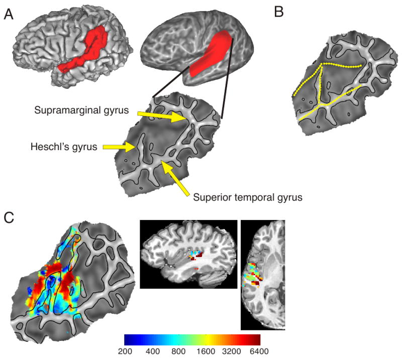
Flattened surface representation. A) Derivation of a flattened patch for a single subject, showing the corresponding area on the original surface. On the patch, gyri are represented with lighter shading and sulci with darker shading. B) Hand drawn boundaries used for group alignment. C) Left hemisphere tonotopy map for a single subject projected on a flattened surface and in volumetric space.
The fMRI data for each subject were analyzed in the volumetric space using Matlab (Mathworks Inc, Natick, MA). Data were pooled across runs and sessions. A general linear model was applied to each voxel time series. Each of the six conditions was represented by a separate regressor. The model baseline was defined as the no-sound condition. Nuisance regressors included baseline, linear, and second-order polynomial terms for each run to reduce the effects of drift in the BOLD signal. Estimates of the mean BOLD signal were calculated for each condition. F-tests were also calculated examining differences across conditions, as well as direct contrasts between high (6400, 3200 Hz), middle (800, 1600 Hz), and low (200, 400 Hz) frequencies. Statistical parametric maps were initially thresholded at p<.01 and then cluster thresholded to correct for multiple comparisons at an alpha level of .05 using the AFNI program AlphaSim (http://afni.nimh.nih.gov/afni). Because no spatial filter was applied to individual subject data, spatial smoothness estimates for the cluster threshold correction were calculated from the residuals of the analyses for each subject using the AFNI program 3dFWHMx. The resulting cluster thresholds varied between subjects, ranging from 20 to 30 mm3. Functional results were projected onto the surface maps using the AFNI program 3dVol2Surf (Figure 3C). Points on the surface map that showed significant differences across frequency (i.e., tonotopy) were then labeled according to the frequency of maximum response. To gain a finer resolution than the six frequencies used in the study, we estimated the frequency response along a continuum using activation levels from multiple conditions. For example, if a point on the surface responds mainly to the 6400 Hz condition it would be labeled with that frequency; however, if the activation levels for both 6400 and 3200 Hz are high then it would be labeled with an intermediate value. Intermediate frequencies of best response at each point on the surface were determined by first selecting a subset of the frequencies that showed greater activation than the mean at that point. For the majority of surface points this consisted of one, two, or three adjacent frequencies. The activation levels for this set of frequencies were normalized to produce a weight vector, which was then multiplied by the corresponding log-transformed frequencies and summed. The resulting number was mapped to a log-scaled color map.
Group alignment and analyses were conducted in the surface space. The flattened surfaces from each subject were aligned to an atlas brain using a nonlinear landmark-based deformation algorithm in Caret (http://brainmap.wustl.edu) (Desai et al., 2005). Landmark-based alignment has been shown to increase spatial precision along the cortical surface of the temporal lobe in comparison to volumetric alignment (Desai et al., 2005; Kang et al., 2004). The atlas brain was a flattened surface from a subject not participating in the study. On each flattened surface the following landmarks (see Figure 3) were identified by hand: HG (for those subjects with a bifurcated HG the more anterior gyrus was chosen), the anterior part of the STG from lateral HG to the anterior boundary of the patch, the posterior part of the STG from lateral HG to the point at which the supramarginal gyrus (SMG) branches off from the STG, the anterior medial boundary of the superior temporal plane lying in the fundus of the Sylvian fissure, and the posterior medial boundary of the superior temporal plane extending to the SMG. The individual subjects’ brains were aligned to the atlas brain by matching the positions of the defined landmarks as closely as possible using a nonlinear fluid deformation. The results of the single subject analyses, including the estimated coefficients for each condition, were transformed onto the atlas surface and spatially smoothed using a 2-mm Gaussian window calculated across the cortical surface. A random effects group analysis examined differences in the estimated coefficients across subjects using one-way ANOVA. Because of the small number of subjects, significance was calculated using a non-parametric permutation test (Nichols and Holmes 2002). To correct for multiple comparisons, cluster-based thresholding was used (Nichols and Holmes 2002), with contiguous clusters calculated based on the connectivity of the surface mesh. The data were initially thresholded at p<.05 and then corrected at an alpha level of .05.
Results
Voxels were identified as having a frequency-selective response if they showed significant differences in activation across the six frequencies as determined by an F test. In all subjects, areas with significant frequency selectivity were confined primarily to the superior temporal plane in both hemispheres (Figure 4). In some subjects frequency-selective activation can be seen in the parietal operculum. Inspection of the data in native volume space, however, showed that this activation is primarily an artifact of the mapping between volume and surface spaces due to partial volume effects (i.e., some voxels span both the upper and lower bank of the sulcus) and small amounts of error in the representation of the surface mesh, which can interfere with accurate separation of functional data from the closely apposed superior temporal plane and parietal operculum.
Figure 4.
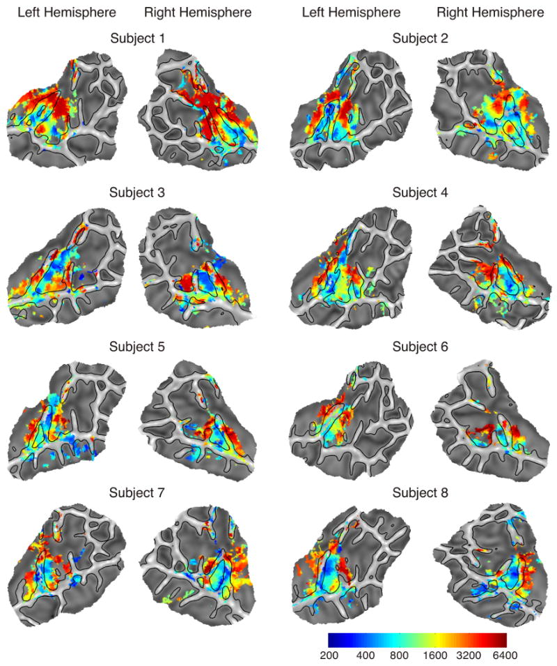
Individual tonotopy maps. Colored regions are areas that showed significant differences across the six conditions (p < .05 corrected). Regions are color-coded according to the frequency with the highest amplitude response.
Individual subjects maps, showing areas with significant frequency selectivity and color-coded according to the frequency of maximum response, are displayed in Figure 4. In all subjects, a prominent low-frequency area with a maximal response to frequencies at 200 or 400 Hz (blue colors) can be observed centrally along the superior temporal plane. Though the exact location of this area varies, it is generally centered either on HG or the sulcus just posterior to HG and extends along an axis roughly parallel to HG. Also present in every subject are two high-frequency areas, located anterior and posterior to the low-frequency zone, that preferentially responded to frequencies at 6400 Hz. Both of the high-frequency areas generally extend more medially than the low-frequency area, and in a few cases (Subjects 1, 7) completely encircle the low-frequency region medially. The anterior high-frequency region typically follows the course of the sulcus anterior to HG (see left hemisphere in Subjects 2, 4, and 5 for clear examples). The posterior high-frequency area is located on the superior temporal plane posterior to HG (planum temporale).
In most of the subjects an additional low-frequency region is present on the lateral posterior STG or at the lateral edge of the planum temporale, just behind the lateral end of the posterior high-frequency zone (see left hemisphere in Subjects 1, 3, 4, 5, 7, 8; right hemisphere in Subjects 2, 5, 6, 7). This region appears to be part of a third, smaller gradient extending along the lateral posterior STG, mainly in the left hemisphere.
The statistical significance of these patterns was investigated by additional contrasts between conditions. The six frequencies were divided into three categories: high (6400, 3200 Hz), medium (1600, 800 Hz), and low (400, 200 Hz) to increase contrast sensitivity. Three contrasts were calculated comparing each frequency category against the other two. Plots of the three contrasts overlaid on the same map are presented for each subject in Figure 5. Both the patterns and spatial extent of these maps are similar to the tonotopic maps presented in Figure 4 and demonstrate that the high, low and intermediate areas identified in those maps represent significant differences in activation across frequencies.
Figure 5.
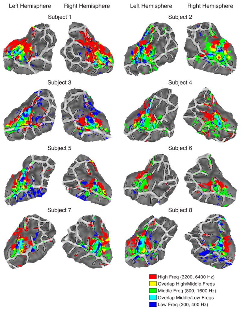
Frequency contrasts. Colored regions are areas that showed significant differences between conditions (p < .05 corrected). Areas showing significant activation for low (200, 400 Hz) over middle (800, 1600 Hz) and high (3200, 6400 Hz) are colored in blue. Areas showing significant activation for middle over low and high are colored in green. Areas showing significant activation for high over low and middle are colored in red. Overlapping areas showing significant activation for both low and middle are colored in cyan and areas showing significant activation for both middle and high are colored in yellow.
These general patterns are seen more clearly on the average group tonotopy map, constructed by landmark-based surface registration of individual maps (Figure 6). A central low-frequency area is seen occupying roughly the lateral half of HG and the transverse temporal sulcus posterior to HG, with its long axis extending parallel to HG. Two prominent high-frequency areas are observed postero-medially and antero-medially to the low-frequency zone. Intermediate-frequency areas are present between the high and low areas, indicating two large, mirror-symmetric frequency gradients extending postero-medially and antero-medially from HG. An additional high-to-low gradient can be discerned along the lateral STG posterior to HG in the left hemisphere, but less prominently in the right hemisphere.
Figure 6.
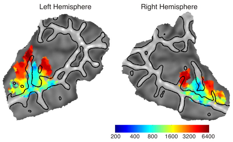
Group tonotopy maps. Colored regions are areas that showed significant differences across the six conditions (p < .05 corrected). Regions are color-coded according to the frequency with the highest amplitude response.
The stability of the tonotopy maps was investigated by examining data from individual sessions. Overall, individual frequency selectivity maps were highly stable across sessions. Figure 7 shows maps for the two subjects who participated in five scanning sessions. Although minor variation in the number of significant voxels and assignment of voxels to a particular frequency can be seen, the cortical location of low- and high-frequency areas as well as the overall pattern is highly reproducible across sessions. The mean between-session correlation coefficient of the tonotopy maps is .834 (SD = 0.083).
Figure 7.
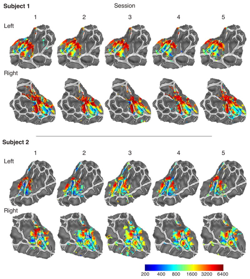
Individual tonotopy maps for two subjects across five different scanning sessions collected on different days.
Differences in frequency selectivity (“tuning bandwidth”) were investigated by comparing the amplitude of the preferred (i.e., highest responding) frequency to the amplitudes of the non-preferred frequencies. We used a methodology similar to the analysis performed by Woods and colleagues (2009). For each subject, the activation levels of each of the six conditions were converted to percent signal change using the rest condition as a baseline. These values were averaged across subjects, and the amplitudes of the six frequencies were normalized by dividing by the amplitude of the frequency with the largest response. Only points on the surface that showed significant frequency selectivity in the group analysis (Figure 6) were analyzed. Points were also excluded if their largest response was to the lowest (200 Hz) or highest (6400 Hz) frequency. The reason for this is that activation levels at the lowest and highest frequencies may not reflect the largest possible response for that brain area, because the area could possibly have larger responses to even lower or higher frequencies that were not included in the experiment. Therefore, normalized values for these regions could be inaccurate. Maps of the mean normalized response are shown in Figure 8. The mean reflects the relative level of the non-preferred frequencies because the preferred frequency is always equal to 1. Lower values represent a greater difference between the preferred and non-preferred frequencies, which is possibly indicative of a sharper tuning for the preferred frequency. A prominent area with relatively small normalized values can be observed centrally in the superior temporal plane just posterior to HG in each hemisphere. Two additional areas with small normalized values can be seen in both hemispheres: one just anterior to HG and another more anterior area lying close to the STG. Areas surrounding these regions show a higher mean normalized response. An inspection of the data without normalization (Figure 8) suggests that these differences across brain areas are driven primarily by an increase in the response to the preferred frequency rather than a decrease in response to the non-preferred frequencies.
Figure 8.
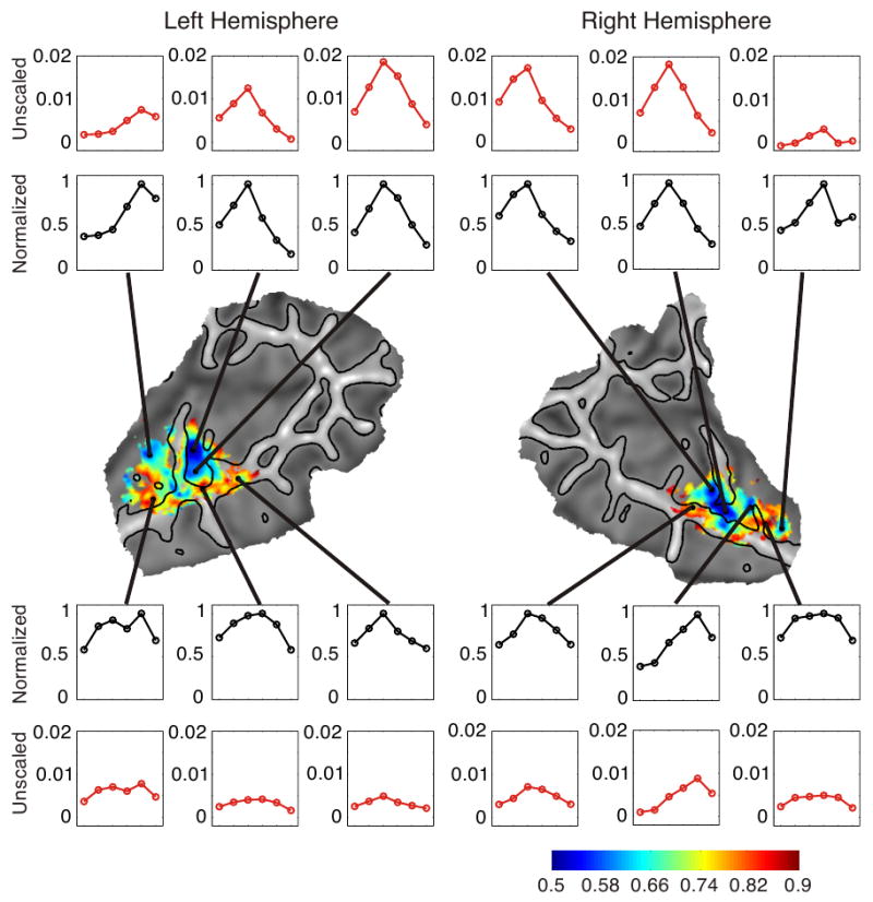
Maps of mean normalized activation levels. Graphs of both the raw (unscaled) and normalized activation levels across conditions are shown for several points in the left and right hemispheres.
Discussion
We observed frequency-selective responses in regions of the superior temporal plane of the human auditory cortex. Two mirror-symmetric tonotopic gradients extended from an area along Heschl's gyrus that was maximally sensitive to lower frequencies. The first gradient extended postero-medially to an area in the planum temporale, and the second extended antero-medially to an area in or near the sulcus anterior to HG. A third, smaller gradient was observed in the lateral posterior aspect of the STG, mainly in the left hemisphere.
These results confirm previous evidence for at least two mirror-symmetric gradients in human auditory cortex (Formisano et al., 2003; Talavage et al., 2004; Woods et al., 2009). The two main gradients in the current study correspond to those observed by Formisano et al. (2003), which those authors described as extending in a caudal-medial to rostral-lateral direction. Example maps in Formisano et al. suggest that these gradients are oriented approximately along the axis of HG, whereas the gradients we observed were perpendicular to the long axis of HG. This discrepancy could be partly due to differences in the stimuli used in the two studies. The highest frequency used by Formisano et al. was 3000 Hz, whereas the current study included frequencies up to 6400 Hz, suggesting that some medial regions anterior to HG that are sensitive to higher frequencies might have been missed in the earlier study. An additional difference is that the activation in Formisano et al. does not extend as far laterally as in the current study, which revealed tonotopic selectivity extending to the outer edge of the STG. This could be due to the broadband nature of our multi-tone stimuli, which may have activated secondary auditory cortex to a greater extent. The two principal gradients in the current study likely correspond to those labeled ‘2 to 1′ and ‘3 to 1′ in the study by Talavage et al. (2004), which are oriented in a similar direction. The posterior (‘3 to 1′) gradient, in particular, appears to correspond closely to the posterior gradient observed in the present study. In both cases the gradient runs perpendicular to the long axis of HG from a posterior high-frequency region on planum temporale to an anterior low-frequency region on HG. The main difference is that Talavage et al. describe their gradients as running along a narrow line between high and low poles, whereas the gradients in the current study might be better characterized as occupying fields bounded by high and low bands. Our results correspond well with the high and low frequency areas identified by Woods et al. (2009). As in the current study, these authors found a single low frequency area centered on HG, bordered anteriorly and posteriorly by two high frequency areas. An additional low frequency area labeled as lateral auditory cortex was also observed by Woods et al. and likely corresponds to the posterior lateral low frequency area observed in the current study. A notable difference is a much larger extent of activation in the anterior high frequency area in the current study. This could be due to differences in the stimuli used in the two studies. The highest frequency band tested by Woods et al. was 3600 Hz, compared to 6400 Hz in the current study. Compared to the stimuli in the current study, the pure tone sequences used by Woods et al. were presented at a slower frequency (4 Hz vs. 10 Hz) and had a narrower bandwidth.
Other investigators reported findings that are clearly not consistent with the current study. For example, a majority of early studies, using only two frequencies, found patterns of low frequency activation on the lateral portion of HG and high frequency activation in medial HG (Bilecen et al., 1998; Lauter et al., 1985; Lockwood et al., 1999; Wessinger et al., 1997). These studies suggested a single principal tonotopic gradient running along the axis of HG, whereas our study and those of Talavage et al. and Woods et al. suggest at least two gradients, at least one of which is oriented perpendicularly to HG. Although there are many differences in methodology between these studies, one that we believe is critical is that the studies reporting gradients perpendicular to HG all used surface-based rather than volume-based analysis. The cortical folding that produces HG causes the high-frequency zones in the sulci posterior and anterior to HG to be physically very close in 3-dimensional space. This physical proximity, together with inter-subject variation in the exact location of the sulci and spatial smoothing used for generating group maps, may have caused these distinct high-frequency areas to blur together. Flattening the superior temporal plane with surface modeling separates these regions and allows a more accurate analysis of topological relations running perpendicular to the gyrus. This could be one reason why the majority of studies using volume-based analysis failed to observe tonotopic gradients perpendicular to HG. In fact, the two volume-based studies that did report tonotopic gradients perpendicular to the long axis of HG used techniques that involved tracing the outline of HG manually in individual subjects, allowing the authors to more carefully characterize differences in frequency response across the gyrus (Schonwiesner, von Cramon, Rubsamen 2002; Talavage et al., 2000). To illustrate this point, Figure 3C shows a tonotopy map for one of the subjects in both surface and volume space. The relatively close proximity of the two high frequency regions located within the sulci bordering HG can be seen in the sagittal and axial views. Finally, the orientation of the gradients with respect to HG depends on the identification of low and high frequency endpoints. The placement of these points could vary a great deal, especially if the spatial extent of the low and high frequency activations is large. This variation could explain why gradients in some studies appear perpendicular to HG while in other studies they appear at a more oblique angle.
The tonotopy maps in our subjects are very similar to those described in macaque monkeys (Figure 1). Early studies of macaque auditory cortex demonstrated two frequency gradients in primary cortex, labeled A1 and R (Merzenich and Brugge 1973). Similar to the current findings, these are mirror-symmetric gradients running in the posterior-anterior axis from high to low to high. Later studies identified an additional primary field anterior to R with its own frequency gradient, called RT (Morel and Kaas 1992), and evidence of tonotopic organization in several secondary belt regions such as AL, ML, RM, MM, and CL (Kusmierek and Rauschecker 2009; Rauschecker, Tian, Hauser 1995; Rauschecker and Tian 2004). In addition to the overall antero-posterior orientation of the core gradients, gradients within A1 and R have been described as oriented diagonally, with higher frequencies represented somewhat more medially and lower frequencies more laterally (Figure 7A) (Bendor and Wang 2008; Kaas and Hackett 2000; Morel and Kaas 1992). Based on these similarities, it is likely that the two gradients observed in the current study encompass two separate regions of cortex homologous to macaque areas A1 and R. It is also likely, however, that these gradients include contiguous belt areas. In the macaque, the lateral belt areas ML and AL and the medial belt areas MM and RM are contiguous with A1 and R, respectively, and have tonotopic gradients that run parallel to those of A1 and R (Kusmierek and Rauschecker 2009; Rauschecker and Tian 2004), with the boundary between core and belt defined by cytoarchitectonic and connectivity patterns rather than tonotopic gradients. Thus, the gradients observed here by fMRI probably include lateral belt regions as well as contiguous core regions. There is little indication in our data of a more anterior core region corresponding to monkey area RT, although a hint of such an anterior gradient can perhaps be seen in the group maps. The lack of frequency-selective activation in this region could be due to low sensitivity to the stimuli used in the current study. Alternatively, it is possible that area RT does not exist in humans. Finally, the smaller gradient observed in the posterior lateral STG likely corresponds to area CL of the macaque, a belt area located posterior to ML that has a gradient running from high frequencies anteriorly to low frequencies posteriorly (Rauschecker and Tian 2004).
Tonotopy in macaque monkey cortex has also been examined using fMRI (Petkov et al., 2006). Examination of the tonotopy maps in the study by Petkov et al. (2006) show a number of similarities with the current data. In their data, a low-frequency band is located in the center of the superior temporal plane, extending perpendicular to the long axis of the STG, similar to low-frequency areas extending along the human HG. A high-frequency region exists immediately posterior to the low-frequency area. In addition, another high-frequency area exists anterior to the low frequency region, though this region appears smaller than the corresponding region in the human cortex. Finally, the fMRI maps in the monkey show another low-frequency area in the far anterior aspect of the superior temporal plane, corresponding to area RT, which was not clearly seen in the current experiment. Based on the divisions of auditory cortex observed in both single unit and fMRI studies, we have drawn tentative boundaries corresponding to locations of homologous regions of the human and macaque auditory cortex in Figure 9. The exact boundary between core and belt cannot be determined based solely on frequency response, thus this line is an estimate guided by the known topographical organization in the macaque and by previous human cytoarchitectonic studies (Fullerton and Pandya 2007; Morosan et al., 2001; Rivier and Clarke 1997). A key feature in orienting this map is the posterior lateral gradient, which most likely corresponds to area CL. In the monkey, this gradient does not extend into adjacent areas; therefore, its boundaries are easily determined. Woods et al. (2009), who show a similar diagram, label this section of cortex as posterior parabelt. We question this interpretation given that there is little evidence for tonotopic organization in the parabelt of monkeys, and recent human cytoarchitectonic data suggest that the parabelt is located more ventrally in the upper bank of the superior temporal sulcus (Fullerton and Pandya 2007). In the posterior medial section of the map, which we label as area CM, there does not appear to be a distinct frequency gradient. This is in agreement with evidence from the macaque suggesting that the majority of neurons in this region respond preferentially to higher than average frequencies (Rauschecker et al., 1997).
Figure 9.
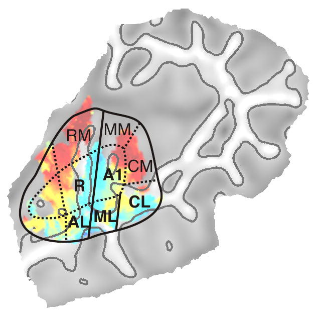
Proposed boundaries of regions in human auditory cortex homologous to regions identified in non-human primate cortex. Solid lines represent boundaries directly determined by activation patterns from the current study. Dotted lines represent proposed boundaries based on previous studies of non-human primates and human cytoarchitectonic studies.
The location of frequency-selective areas was stable across sessions. However, some inter-session variability was seen in the number of significantly activated voxels and their preferred frequency. Some of this variance can be attributed to differences across sessions in the amount of head movement and other artifacts. Another possible source of variance is physiologic state changes such as alterations in attention and alertness. The maps in our study did show a high degree of variability across subjects and across hemispheres. For example, the location of the low-frequency border between the two gradients varied in relation to HG. This observation supports previous studies of the cytoarchitecture of human auditory cortex, which reported variance in the position of primary auditory cortex relative to gyral and sulcal landmarks (Hackett, Preuss, Kaas 2001; Rademacher et al., 2001).
Topographical variation in the ratio of the BOLD response to preferred and non-preferred frequencies was found in both hemispheres. These results are in agreement with Woods et al. (2009), who performed a similar analysis and found a larger difference between preferred and non-preferred frequencies in a central region of auditory cortex and smaller differences in more lateral areas. Our results also showed additional regions with large differences between preferred and non-preferred frequencies in more anterior areas of auditory cortex, which were not apparent in the Woods et al. study. The relatively stronger responses to preferred compared to non-preferred frequencies could be interpreted as reflecting narrower tuning bandwidths in these regions. These regions may thus correspond to primary core areas, which have been found in non-human primates to have narrower tuning curves than more lateral regions (Rauschecker et al., 1995). We note, however, that these patterns generally appear to be correlated with the overall strength of the response. That is, increased differences in the response to the preferred versus non-preferred frequencies are driven primarily by increases in response to the preferred frequency rather than decreases in the response to the non-preferred frequencies. In addition to broader tuning, these more lateral regions thus appear to be generally less responsive to tonal stimuli that lack complex spectrotemporal features such as those found in speech and other naturally occurring sounds.
Acknowledgments
Supported by National Institutes of Health grants R01-NS33576, R01-DC006287, F32-DC007024, T32-MH019992, and M01-RR00058.
Footnotes
Publisher's Disclaimer: This is a PDF file of an unedited manuscript that has been accepted for publication. As a service to our customers we are providing this early version of the manuscript. The manuscript will undergo copyediting, typesetting, and review of the resulting proof before it is published in its final citable form. Please note that during the production process errors may be discovered which could affect the content, and all legal disclaimers that apply to the journal pertain.
References
- Bendor D, Wang X. Neural response properties of primary, rostral, and rostrotemporal core fields in the auditory cortex of marmoset monkeys. Journal of Neurophysiology. 2008;100(2):888–906. doi: 10.1152/jn.00884.2007. [DOI] [PMC free article] [PubMed] [Google Scholar]
- Bilecen D, Scheffler K, Schmid N, Tschopp K, Seelig J. Tonotopic organization of the human auditory cortex as detected by BOLD-FMRI. Hearing Research. 1998;126(12):19–27. doi: 10.1016/s0378-5955(98)00139-7. [DOI] [PubMed] [Google Scholar]
- Desai R, Liebenthal E, Possing ET, Waldron E, Binder JR. Volumetric vs. surface-based alignment for localization of auditory cortex activation. NeuroImage. 2005;26(4):1019–1029. doi: 10.1016/j.neuroimage.2005.03.024. [DOI] [PubMed] [Google Scholar]
- Formisano E, Kim DS, Di Salle F, van de Moortele PF, Ugurbil K, Goebel R. Mirror-symmetric tonotopic maps in human primary auditory cortex. Neuron. 2003;40(4):859–869. doi: 10.1016/s0896-6273(03)00669-x. [DOI] [PubMed] [Google Scholar]
- Fullerton BC, Pandya DN. Architectonic analysis of the auditory-related areas of the superior temporal region in human brain. The Journal of Comparative Neurology. 2007;504(5):470–498. doi: 10.1002/cne.21432. [DOI] [PubMed] [Google Scholar]
- Hackett TA, Preuss TM, Kaas JH. Architectonic identification of the core region in auditory cortex of macaques, chimpanzees, and humans. The Journal of Comparative Neurology. 2001;441(3):197–222. doi: 10.1002/cne.1407. [DOI] [PubMed] [Google Scholar]
- Kaas JH, Hackett TA. Subdivisions of auditory cortex and processing streams in primates. Proceedings of the National Academy of Sciences of the United States of America. 2000;97(22):11793–11799. doi: 10.1073/pnas.97.22.11793. [DOI] [PMC free article] [PubMed] [Google Scholar]
- Kang X, Bertrand O, Alho K, Yund EW, Herron TJ, Woods DL. Local landmark-based mapping of human auditory cortex. NeuroImage. 2004;22:1657–1670. doi: 10.1016/j.neuroimage.2004.04.013. [DOI] [PubMed] [Google Scholar]
- Kosaki H, Hashikawa T, He J, Jones EG. Tonotopic organization of auditory cortical fields delineated by parvalbumin immunoreactivity in macaque monkeys. The Journal of Comparative Neurology. 1997;386(2):304–316. [PubMed] [Google Scholar]
- Kusmierek P, Rauschecker JP. Functional specialization of medial auditory belt cortex in the alert rhesus monkey. Journal of Neurophysiology. 2009 doi: 10.1152/jn.00167.2009. [DOI] [PMC free article] [PubMed] [Google Scholar]
- Langers DR, Backes WH, van Dijk P. Representation of lateralization and tonotopy in primary versus secondary human auditory cortex. NeuroImage. 2007;34(1):264–273. doi: 10.1016/j.neuroimage.2006.09.002. [DOI] [PubMed] [Google Scholar]
- Lauter JL, Herscovitch P, Formby C, Raichle ME. Tonotopic organization in human auditory cortex revealed by positron emission tomography. Hearing Research. 1985;20(3):199–205. doi: 10.1016/0378-5955(85)90024-3. [DOI] [PubMed] [Google Scholar]
- Lockwood AH, Salvi RJ, Coad ML, Arnold SA, Wack DS, Murphy BW, Burkard RF. The functional anatomy of the normal human auditory system: Responses to 0.5 and 4.0 kHz tones at varied intensities. Cerebral Cortex (New York, NY: 1991) 1999;9(1):65–76. doi: 10.1093/cercor/9.1.65. [DOI] [PubMed] [Google Scholar]
- Merzenich MM, Brugge JF. Representation of the cochlear partition of the superior temporal plane of the macaque monkey. Brain Research. 1973;50(2):275–296. doi: 10.1016/0006-8993(73)90731-2. [DOI] [PubMed] [Google Scholar]
- Morel A, Kaas JH. Subdivisions and connections of auditory cortex in owl monkeys. The Journal of Comparative Neurology. 1992;318(1):27–63. doi: 10.1002/cne.903180104. [DOI] [PubMed] [Google Scholar]
- Morel A, Garraghty PE, Kaas JH. Tonotopic organization, architectonic fields, and connections of auditory cortex in macaque monkeys. The Journal of Comparative Neurology. 1993;335(3):437–459. doi: 10.1002/cne.903350312. [DOI] [PubMed] [Google Scholar]
- Morosan P, Rademacher J, Schleicher A, Amunts K, Schormann T, Zilles K. Human primary auditory cortex: Cytoarchitectonic subdivisions and mapping into a spatial reference system. NeuroImage. 2001;13(4):684–701. doi: 10.1006/nimg.2000.0715. [DOI] [PubMed] [Google Scholar]
- Nichols TE, Holmes AP. Nonparametric permutation tests for functional neuroimaging: A primer with examples. Human Brain Mapping. 2002;15(1):1–25. doi: 10.1002/hbm.1058. [DOI] [PMC free article] [PubMed] [Google Scholar]
- Petkov CI, Kayser C, Augath M, Logothetis NK. Functional imaging reveals numerous fields in the monkey auditory cortex. PLoS Biology. 2006;4(7):e215. doi: 10.1371/journal.pbio.0040215. [DOI] [PMC free article] [PubMed] [Google Scholar]
- Rademacher J, Morosan P, Schormann T, Schleicher A, Werner C, Freund HJ, Zilles K. Probabilistic mapping and volume measurement of human primary auditory cortex. NeuroImage. 2001;13(4):669–683. doi: 10.1006/nimg.2000.0714. [DOI] [PubMed] [Google Scholar]
- Rauschecker JP, Tian B. Processing of band-passed noise in the lateral auditory belt cortex of the rhesus monkey. Journal of Neurophysiology. 2004;91(6):2578–2589. doi: 10.1152/jn.00834.2003. [DOI] [PubMed] [Google Scholar]
- Rauschecker JP, Tian B, Hauser M. Processing of complex sounds in the macaque nonprimary auditory cortex. Science (New York, NY) 1995;268(5207):111–114. doi: 10.1126/science.7701330. [DOI] [PubMed] [Google Scholar]
- Rauschecker JP, Tian B, Pons T, Mishkin M. Serial and parallel processing in rhesus monkey auditory cortex. The Journal of Comparative Neurology. 1997;382(1):89–103. [PubMed] [Google Scholar]
- Rivier F, Clarke S. Cytochrome oxidase, acetylcholinesterase, and NADPH-diaphorase staining in human supratemporal and insular cortex: Evidence for multiple auditory areas. NeuroImage. 1997;6(4):288–304. doi: 10.1006/nimg.1997.0304. [DOI] [PubMed] [Google Scholar]
- Schonwiesner M, von Cramon DY, Rubsamen R. Is it tonotopy after all? NeuroImage. 2002;17(3):1144–1161. doi: 10.1006/nimg.2002.1250. [DOI] [PubMed] [Google Scholar]
- Talavage TM, Ledden PJ, Benson RR, Rosen BR, Melcher JR. Frequency-dependent responses exhibited by multiple regions in human auditory cortex. Hearing Research. 2000;150(12):225–244. doi: 10.1016/s0378-5955(00)00203-3. [DOI] [PubMed] [Google Scholar]
- Talavage TM, Sereno MI, Melcher JR, Ledden PJ, Rosen BR, Dale AM. Tonotopic organization in human auditory cortex revealed by progressions of frequency sensitivity. Journal of Neurophysiology. 2004;91(3):1282–1296. doi: 10.1152/jn.01125.2002. [DOI] [PubMed] [Google Scholar]
- Wessinger CM, Buonocore MH, Kussmaul CL, Mangun GR. Tonotopy in human auditory cortex examined with functional magnetic resonance imaging. Human Brain Mapping. 1997;5:18–25. doi: 10.1002/(SICI)1097-0193(1997)5:1<18::AID-HBM3>3.0.CO;2-Q. [DOI] [PubMed] [Google Scholar]
- Woods DL, Stecker GC, Rinne T, Herron TJ, Cate AD, Yund EW, Liao I, Kang X. Functional maps of human auditory cortex: Effects of acoustic features and attention. PloS One. 2009;4(4):e5183. doi: 10.1371/journal.pone.0005183. [DOI] [PMC free article] [PubMed] [Google Scholar]