

Abstract
During the crossing of the place field of a pyramidal cell in the rat hippocampus, the firing phase of the cell decreases with respect to the local theta rhythm. This phase precession is usually studied on the basis of data in which many place field traversals are pooled together. Here we study properties of phase precession in single trials. We found that single-trial and pooled-trial phase precession were different with respect to phase-position correlation, phase-time correlation, and phase range. Whereas pooled-trial phase precession may span 360°, the most frequent single-trial phase range was only ∼180°. In pooled trials, the correlation between phase and position (r = −0.58) was stronger than the correlation between phase and time (r = −0.27), whereas in single trials these correlations (r = −0.61 for both) were not significantly different. Next, we demonstrated that phase precession exhibited a large trial-to-trial variability. Overall, only a small fraction of the trial-to-trial variability in measures of phase precession (e.g., slope or offset) could be explained by other single-trial properties (such as running speed or firing rate), whereas the larger part of the variability remains to be explained. Finally, we found that surrogate single trials, created by randomly drawing spikes from the pooled data, are not equivalent to experimental single trials: pooling over trials therefore changes basic measures of phase precession. These findings indicate that single trials may be better suited for encoding temporally structured events than is suggested by the pooled data.
Introduction
The temporal relation of action potentials of CA1 pyramidal cells to the theta oscillation in the local field potential (LFP) is one of the few known examples of correlation coding in the brain (Dayan and Abbott, 2001). To relate spike times to the LFP, each spike is assigned a theta phase between 0° and 360°, where 0° corresponds to the trough of the theta oscillation. The CA1 spike phases decrease from theta cycle to theta cycle during the crossing of the place field of a pyramidal cell (O'Keefe and Recce, 1993). Hence, the spike phase is negatively correlated with both the position of the animal within the place field (“phase-position correlation”) and the time that has passed since the animal entered the place field (“phase-time correlation”) (Huxter et al., 2003). This phenomenon is called phase precession.
Phase precession interestingly leads in effect to the temporal compression of behavioral sequences: within one theta cycle (∼125 ms), the order of activity among a group of place cells with overlapping place fields corresponds to the order in which the animal crosses the place fields (Skaggs et al., 1996); in particular, the spatial distances between place field centers are encoded in the time lag between the activity of respective place cells within one theta cycle (Dragoi and Buzsáki, 2006; Diba and Buzsáki, 2008; Lenck-Santini and Holmes, 2008). Thus, phase precession allows the compression of temporal sequences from a behavioral timescale of seconds to the timescale of a theta cycle (Mehta et al., 2002), a timescale relevant for spike-timing-dependent plasticity (Levy and Steward, 1983; Gerstner et al., 1996; Markram et al., 1997; Bi and Poo, 1998; Kempter et al., 1999). This compression could provide a basic mechanism for a neural representation of temporal order relevant for episodic memory (Buzsáki, 2005).
Phase precession is usually studied on the basis of data in which many place field traversals are pooled together (O'Keefe and Recce, 1993; Skaggs et al., 1996; Huxter et al., 2003). However, functional hypotheses on phase precession, including temporal coding (Harris et al., 2002; Mehta et al., 2002; Huxter et al., 2003; Leibold et al., 2008; Thurley et al., 2008), sequence learning or recall (Hasselmo and Eichenbaum, 2005; Lisman et al., 2005), and spatial navigation (Burgess et al., 1994; Koene et al., 2003; Lengyel et al., 2005), rely on experiences occurring in single trials. Pooling data over trials may lead to a biased estimate of properties of phase precession and neglects potential trial-to-trial variability.
In this study, we analyze properties of phase precession in single trials and compare them with properties of pooled-trial phase precession. We find that phase-position correlations, phase-time correlations, and phase ranges are different in single trials and pooled trials. Furthermore, we quantify trial-to-trial variability in phase precession and examine whether external factors, such as a variable running speed, can account for it. Finally, we demonstrate, on the basis of surrogate data, that pooling phase precession over trials changes basic measures of phase precession. Our findings indicate that single trials may be better suited for encoding temporally structured events, such as episodic memories, than is suggested by the pooled data.
Materials and Methods
General
Experimental data has been used in a different study (Diba and Buzsáki, 2008) in which experimental procedures have been described in detail. Briefly, three male Sprague Dawley rats were trained to run back and forth ∼20 times on a linear track (170 cm long) to retrieve water rewards at both ends. Then the track was shortened (to 100 cm) and the rat ran another ∼20 times back and forth. Changes in place field activity attributable to shortening of the track have been described in detail by Diba and Buzsáki (2008). All protocols were approved by the Institutional Animal Care and Use Committee of Rutgers University. After learning the task, the rats were implanted with 32- and/or 64-site silicon probes in the left dorsal hippocampus under isoflurane anesthesia. The silicon probes, consisting of four or eight individual shanks (spaced 200 μm apart) of eight staggered recording sites (20 μm spacing) (Csicsvari et al., 2003), were lowered to CA1 and CA3 pyramidal cell layers. After recovery from surgery (∼1 week), the animals were tested again on the track. The position of the animals was tracked with a light-emitting diode and later linearized along the long axis of the track. For this study, all units and LFPs were taken from CA1 recording sites. Spikes that occurred near reward sites were excluded from the analysis by checking whether the position of the rat corresponds to one of the two reward platforms. This exclusion was done to ensure that spikes during non-theta states, e.g., sharp wave-ripple events during sequence replay (Foster and Wilson, 2006; Diba and Buzsáki, 2007), did not enter the analysis. All major results were reproduced in an analysis, including spikes at reward sites. We also used the running speed of the rat as a criterion for spike selection (see below).
Place fields
Place fields were determined by a firing-rate criterion. The peak firing rate had to be at least 2 Hz. The borders of the place fields were set at the location where the firing rate dropped below 10% of the place field peak firing rate. All results were also reproduced with a 20% criterion. Spikes outside the place fields were discarded. For each cell, place fields were determined separately for the long and short tracks and for leftward and rightward runs along the linear tracks. Place fields were also determined separately for each recording session. For rat 1, there were 12 recording sessions yielding 118 place fields, for rat 2, there were 11 sessions and 158 place fields, and for rat 3, there were 33 sessions and 890 place fields. In total, 1166 place fields with overall 20,602 single trials were analyzed. Animal position within a place field was normalized to values between 0 and 1. Only CA1 place fields with a significant negative linear correlation of at least 0.4 between spike phase and relative position in the place field were used in the analysis.
A trial consisted of a single crossing of a place field. In some trials, if animals stopped within a place field, then theta oscillations in the LFP typically disappeared and the theta phase of a spike could not be reliably determined. Therefore, spikes that occurred when the instantaneous running speed was smaller than 10 cm/s were discarded. In addition, trials in which the average running speed was smaller than 10 cm/s were excluded from both the single-trial and pooled-trial analyses. Furthermore, single trials were required to span at least two theta cycles, with at least three spikes in total, to be included in the analysis. However, exclusion of such trials did not affect the overall results.
Quantifying phase precession
For spike phase estimation, the CA1 LFP was bandpass filtered between 6 and 10 Hz and the Hilbert transform was applied. We always refer to the LFP in the CA1 pyramidal cell layer theta, and 0° corresponds to troughs in the filtered LFP.
Correlation coefficient.
Phase precession was quantified with a linear correlation coefficient to allow comparison with previous studies. To reduce problems arising from the circularity of phase, for each place field, the phase was shifted to minimize the linear correlation coefficient (O'Keefe and Recce, 1993; Mehta et al., 2002).
Phase range.
Phase ranges of spikes were estimated by fitting a line in phase-position plots using a circular–linear fit described below (for alternative methods, see supplemental Results, available at www.jneurosci.org as supplemental material). The slope of the line times the spatial range of the trial (defined below) determined the single-trial phase range. For the estimation of the range of phase precession, the slope was limited to the interval [−4π, 0]. This restriction avoided fitting lines with arbitrary high slopes that could cross all data points. Positive slopes were also excluded because we were interested in the range of phase precession with negative values. For example, a slope of −2π and a spatial range of 0.5 yields a phase range of −π. For analyses other than the phase range (e.g., estimating slope or phase offset), the slope was limited to the interval [−4π,4π].
Phase offset and slope.
To avoid inappropriate linear fits (see Fig. 1 and supplemental Fig. 1, column 5, row 4, available at www.jneurosci.org as supplemental material), a circular–linear fit (see below) was used to estimate the slope and the phase offset of phase precession (see Figs. 3–5). The phase offset was assessed by the phase value of the fitted line at relative position zero.
Figure 1.

Pooled-trial (A) and single-trial (B) phase precession. Each dot represents a spike at a certain relative position in the place field (x-axis, normalized position with range from 0 to 1) at a certain theta phase in degrees (y-axis, full range of 360°; unlabeled tick at 180°). The top row shows five example cells with phase precession pooled over up to 20 trials. The gray lines are linear fits, and the inset numbers give corresponding correlation coefficients. The four bottom rows depict robust phase precession in sample single trials from the respective cells.
Figure 3.

Variability of phase precession. We considered variability of the measures phase-position correlation (A), phase offset (B), slope (C), and phase range (D) for single trials (A1–D1) and pooled trials (A2–D2). Insets in A1–D1 show an example single trial (same as in Fig. 1, column 3, row 4) with the corresponding values of the measures. Note that considerable variability exists in all four measures. Positive slopes fitted to single trials (C1) can be attributable to bimodal phase distributions (Kjelstrup et al., 2008) (supplemental Fig. 1, available at www.jneurosci.org as supplemental material). A3–D3, Trial-to-trial variability within randomly selected example place fields. Single-trial values of the four measures (black bars) are shown for 60 place fields (rat 1, place field index 1–20; rat 2, 21–40; rat 3, 41–60). Large variability exists within a given place field, whereas the variability of pooled-trial values (gray circles) is comparatively small across place fields.
Figure 4.

Properties and correlations between properties of single trials. A, Properties. Values were derived from place-field crossings, i.e., from the time between the first and the last spike within the place field. Note that, for some properties, few values were outside the range shown here (0.36% of the values for number of spikes, 0.13% for firing rate, and 1.6% for number of theta cycles) and were thus collapsed into the last histogram bin. Trials with average running speeds below 10 cm/s, less than three spikes, or less than two theta cycles were excluded from the analysis. B, Matrix of correlation coefficients of pairs of single-trial properties. Shown are correlations between phase-position correlation (R), slope (Slope), phase offset (Offset), phase range (PhaRa), spatial range (SpaRa), number of spikes (Spikes), mean firing rate (Rate), number of theta cycles (Cycles), running speed (Speed), theta frequency (Freq), theta amplitude (Amp), skewness (Skew), and within-session trial index (Trial). In the top right triangle, correlation coefficients are color coded; in the bottom left triangle, numerical values are given. Highly significant correlation coefficients (p < 0.0001) are written in black, and others are in gray. Note that, for the circular variable phase offset, a circular–linear correlation coefficient is shown.
Figure 5.
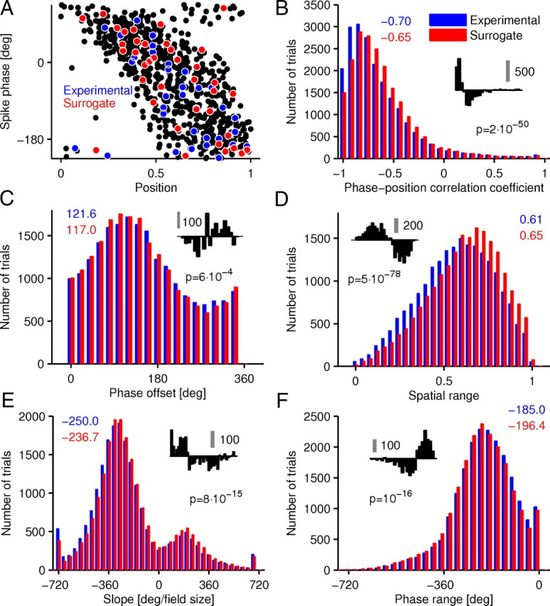
Surrogate single trials. A, Illustration of the method to create surrogate single trials. Black dots represent spikes from an example place field (rat 2, cell 195). Blue dots indicate spikes from a single trial (phase-position correlation, r = −0.49). Red dots are spikes randomly picked from the population of the black dots with the spike number being equal to the blue dots. Thus, the red dots form a surrogate single trial (phase-position correlation, r = −0.59). B–F, Distributions of single-trial measures from surrogate and experimental trials. Colored numbers give median value for experimental and surrogate distribution, respectively. For phase offset, the circular mean is given instead of the median. Black numbers give p values for Kolmogorov–Smirnov tests. Insets show the difference between the distributions, and the gray scale bars give the respective number of trials. Note that experimental trials have stronger phase-position correlations than surrogate trials (B).
Circular–linear fit.
Given a random sample of data (ϕ1, x1), …, (ϕn, xn) on the surface of a cylinder where ϕj is an angular and xj is a linear measurement (j = 1, …, n), a linear model was fitted:
 |
The two parameters of this model are the slope a and the phase offset ϕ0. The model allows prediction of the mean angle Φ given the position X. To obtain an estimate of the slope a, the mean resultant length,
 |
was maximized. Because it is independent of ϕ̂0, the estimate â of the slope a is â = arg maxa R(a), which demands numerical methods. The estimate ϕ̂0 for the phase offset then follows from (Gould, 1969; Fisher, 1995)
 |
where the function arctan* is the quadrant-specific inverse of the tangent.
Other single-trial properties
In addition to the above measures that quantify phase precession, we calculated nine other single-trial properties (see Fig. 4).
We took into account (1) the number of spikes and (2) the firing rates within single trials. The firing rates were determined by the number of spikes within the place field minus 1, divided by the time passed between the first and last spike in that run. (3) Theta cycles per trial were counted by the number of theta cycles between the first and the last spike of the trial, including the border cycles. Theta cycles started and ended at the peaks of the filtered LFP. (4) Running speed was estimated by the distance between the animal position at the first and the last spike divided by the time passed between the first and last spike in the place field. Furthermore, each spike was assigned a theta frequency and amplitude with respect to the LFP at the time the spike occurred. Trial-specific (5) theta frequency estimates were obtained by calculating the mean overall spikes in a trial. (6) Single-trial skewness was determined with respect to the relative location of the spikes within the place field. Formally, sample skewness is defined as
 |
where xi denotes the relative location of spike i in the place field, m is the number of spikes in a single trial, and  x
x is the sample mean. Negative skewness corresponds to a greater number of spikes toward the end of the place field. (7) The spatial range is the fraction of the place field covered by a single trial. It was calculated as the difference between the relative position in the place field of the first and the last spike in a trial. (8) The theta amplitude was estimated for each spike as the difference between the maximum and the minimum of the filtered LFP signal in the corresponding theta cycle divided by two. The mean overall amplitude values of all spikes in a trial yielded the trial-specific theta amplitudes. Finally, we considered (9) the trial index (lap number) in a recording session.
Variance decomposition
Variance decomposition was used to determine the contributions of within-cell variance and between-cell variance to the total variance present in a population of N cells. For example, if the firing rate of a place cell is similar across trials but very different across cells, the within-cell variance will be small and the between-cell variance large. Formally, the population variance σPop2 can be decomposed into the sum of within-cell and between-cell variances: σPop2 = σwithin2 + σbetween2. The within-cell variance σwithin2 is given by the weighted mean of cell-specific variances σn2 for n = 1, …, N cells. The weighting occurs according to the number of trials Tn in cell n and the population mean number of trials T̄:
 |
 |
The cell-specific variance is
 |
with the single-trial property xn,t of cell n in trial t and a cell-specific mean
 |
. The between-cell variance is given by the weighted variance across cell means:
 |
with the population mean
 |
.
For the circular variable “phase offset,” we used a variance decomposition method based on the mean resultant length (Harrison et al., 1986):
 |
with the phase offset ϕn,t in cell n and trial t, and the circular population mean ϕ̄ of the phase offset. The weighted average of cell-specific variation measures is given by
 |
with the cell-specific mean resultant length
 |
and the cell-specific circular mean ϕ̄n. The measure of the population variance was decomposed into between and within variance through
 |
where [r̄2 − r2] is the measure for the circular between-cell variance, and [1 − r̄2] the measure for the circular within-cell variance.
Correlation analyses
Shown correlation coefficients are usually Pearson's product-moment correlation coefficients. For the correlation analyses (see Fig. 4B) that included the phase offset and another linear variable, a circular–linear correlation coefficient was calculated instead.
The correlation analyses can be done in two different ways. For each place field, the correlations between pairs of single-trial properties are calculated, and afterward an average correlation across the population is determined; alternatively, pairs of single-trial properties are pooled across cells and animals, and then the correlation coefficient is calculated for the pooled data. For the analyses in Figure 4B, the latter method was used. The matrix for the other method is shown in supplemental Figure 5 (available at www.jneurosci.org as supplemental material). In most cases, the two methods yielded comparable results.
Surrogate data
Surrogate single trials were generated by randomly drawing spikes from the pooled place field data. The phase and position of these spikes were kept. These surrogate single trials had the same number of spikes as the corresponding experimental trials. In the basic version (used in Fig. 5), spikes were drawn without replacement: each spike from the place field could only be used in one surrogate trial. We also created surrogate methods with additional constraints to closer match the properties of experimental trials (see supplemental Results, available at www.jneurosci.org as supplemental material).
Results
Experimental data on phase precession were obtained from three rats running back and forth on a linear track to retrieve water rewards at both ends. Electrophysiological recordings were done in the hippocampal CA1 region using silicon probes. To quantify phase precession in single trials, we used spikes from CA1 pyramidal cells with place fields on the linear track together with the LFP in the CA1 pyramidal cell layer.
Differences between single-trial and pooled-trial phase precession
Single trials exhibit phase precession
Phase precession is commonly quantified through the correlation coefficient between spike phase and animal position; in previous approaches, data from different trials (place field traversals) was pooled. Figure 1A shows five example place fields exhibiting phase precession, evident from a significant negative correlation between spike phase and animal position. In addition, examples of single trials from the same cells are shown (Fig. 1B). For quantitative analyses, we determined phase-position and phase-time correlation coefficients for single trials and pooled trials of 1166 place fields.
Phase-position correlations
The distribution of phase-position correlation coefficients of our 20,602 single trials contained a large fraction with negative values (mean ± SEM, −0.61 ± 0.0023) (Fig. 2A). Furthermore, significant correlation coefficients were almost exclusively negative (−0.75 ± 0.0015). Trials were labeled significant when the p value of the linear correlation was below 0.05 and the corresponding trial had at least five spikes. The distribution of pooled-trial correlation coefficients (−0.58 ± 0.0032) was different from that of the single-trial correlation coefficients.
Figure 2.

Correlation coefficients for pooled-trial and single-trial phase precession. A, Histograms of correlation coefficients of spike phase with relative position in the place field. Single trials show stronger negative correlations than pooled trials. Only place fields with a pooled-trial phase-position correlation of at least −0.4 were included in the analysis (see Materials and Methods). B, Histograms of correlation coefficients of spike phase with time passed since the animal entered the place field. Correlations are considerably strong in single trials but weak in pooled trials. The histograms of single trials (n = 20,602) in A and B include the shown significant trials (n = 11,516 for phase position and n = 11,984 for phase time). C, Correlation coefficients between position and time passed since the animal entered the place field illustrate strong single-trial but weak pooled-trial correlations. Note that the last bin contains values in the interval [0.9, 1.0].
Phase-time correlations
Similar to the phase-position correlations, the distribution of single-trial phase-time correlations had a large fraction with negative values (−0.61 ± 0.0023), especially the significant ones (−0.74 ± 0.0015) (Fig. 2B). The distribution of pooled trials (−0.27 ± 0.0058) was different from that of single trials and reflected a weaker mean correlation. Because in time-based measures pooling faster and slower trials combines “steep” and “flat” phase precession slopes, this likely produced a weaker phase-time correlation compared with the phase-position correlation. In line with this argument, the SD of single-trial running speed across trials in a place field correlated with the phase-time correlation in pooled trials (r = 0.31; p = 5 × 10⁻²⁷). Also, the difference between the phase-time and the phase-position correlations correlated with the SD of the running speed (r = 0.23; p = 7 × 10⁻¹⁵). Thus, place fields with a strong negative pooled phase-time correlation were those which the rat usually crossed with similar running speeds. Moreover, we found that the position of the animal and the time that has passed since the animal entered the place field were more strongly correlated in single trials (0.98 ± 0.0005) than in pooled trials (0.47 ± 0.0081) (Fig. 2C). Comparing the distributions of correlation coefficients for single trials in Figure 2, A and B, we did not find a significant difference between phase-position and phase-time correlations (Kolmogorov–Smirnov test, p = 0.60).
Trial-to-trial variability
How does single-trial phase precession vary from trial to trial? To answer this question, we specified several measures for phase precession. Besides the phase-position correlation, we also used the phase offset, the slope, and the phase range to quantify phase precession (see Materials and Methods) (Fig. 3A1–D1, insets).
Variability of measures for phase precession
The overall distributions of phase-position correlation, phase offset, slope, and phase range suggest that there is substantial variability in the overall population of single trials (Fig. 3A1–D1). These distributions were different from the corresponding distributions from pooled trials (Fig. 3A2–D2). In particular, we found single-trial phase ranges of −191.2 ± 0.8° (mean ± SEM) (Fig. 3D1), which were considerably shorter than the pooled-trial phase ranges of −296.8 ± 3.2° (Fig. 3D2). This difference was mostly attributable to the fact that only a fraction of the full place field was covered in most single trials (for details, see supplemental Results, available at www.jneurosci.org as supplemental material). Moreover, the relative position of the first spike in the field in a trial correlated weakly with the theta phase of this spike (r = −0.06) but stronger with the phase offset of that trial (r = 0.20). Thus, place cells started firing at a similar phase even if the first spike in a trial occurred at a later position in the place field, which contributes to the variability of phase precession.
What is the origin of the observed variability? In general, all trials from the same cell could have the same phase-position correlation, phase offset, slope, and phase range. In this case, all variability originates from variability between cells and not from variability within cells. Alternatively, the mean values for the measures of phase precession could be the same for all cells, but, in each cell, there may be a lot of variability across trials. In that case, variability originates from within cells and not from variability between cells.
We found that the distributions reflect trial-to-trial variability rather than variability between cells. To quantify the trial-to-trial variability, we determined the contributions of within- and between-cell variance in our dataset through variance decomposition (see Materials and Methods). We identified that indeed a large fraction of the variance originated from within-cell variance: 85% for the phase-position correlation, 72% for the offset, 87% for the slope, and 74% for the phase range. We illustrate this result for 60 sample place fields in Figure 3A3–D3. In conclusion, considerable trial-to-trial variability of phase precession exists in the phase-position correlation, phase offset, slope, and phase range.
Evidence for inherent trial-to-trial variability
Given the trial-to-trial variability with respect to phase-position correlation, phase offset, slope, and phase range, it is important to ask whether the variability in any of these measures is inherent or is controlled by an external factor. For example, does “running speed” determine the slope of phase precession? Does the phase-position correlation become stronger over trials? To answer such questions, we determined the extent to which measures of phase precession can be predicted from a linear model based on other single-trial properties.
We examined the following single-trial properties (Fig. 4A) (median ± SD): (1) number of spikes (10 ± 8.7 spikes), (2) firing rate (18.2 ± 12.2 Hz), (3) number of theta cycles (5.0 ± 5.4), (4) running speed of the rat (68.2 ± 22.6 cm/s), (5) theta frequency (8.3 ± 0.4 Hz), and (6) skewness (−0.08 ± 0.6). Furthermore, we considered (7) the spatial range (0.61 ± 0.21) (supplemental Fig. 2A, available at www.jneurosci.org as supplemental material), (8) the theta amplitude, and (9) the trial index, or lap number, in that recording session (data not shown). Together with the four measures of phase precession in Figure 3, we have 13 properties. For each pair of properties, we calculated the correlation coefficient (Fig. 4B) (see Materials and Methods). We found, for example, a highly significant (p = 1.6 × 10−73) but weak (r = −0.13) correlation between the running speed and the phase-position correlation coefficient (supplemental Fig. 5A, available at www.jneurosci.org as supplemental material). Therefore, assuming a linear relationship, running speed alone could explain only r2 = 1.69% of the variance in the phase-position correlation in single trials. None of the nine examined single-trial properties exhibited a strong correlation with the phase-position correlation, the slope, or the offset, although these three measures were correlated to each other to some extent. The phase range correlated with the spatial range (see supplemental Results, available at www.jneurosci.org as supplemental material), the number of theta cycles, and the number of spikes. Thus, more theta cycles in a trial allow a larger phase range as well as a larger number of spikes. We conclude that, according to this analysis, most of the trial-to-trial variability in phase precession is inherent unless it is controlled by another factor that we have not identified.
Single trials are not equivalent to randomly drawn spikes from the pooled data
So far, we have revealed the existence of substantial trial-to-trial variability in phase precession, which could not be explained by the other single-trial properties. A large fraction of this variability appears to be independent of these properties. Pooling trials with different running speeds, etc., would be valid if all spikes/trials are drawn from the same joint probability distribution of spike phase and position. However, it is unknown whether the pooled data actually serves as a proper predictor for single trials.
If all spikes from a given place field are drawn from the same joint probability distribution, this distribution can be estimated by the pooled data. Furthermore, randomly drawn spikes from the pooled data should have similar properties as experimental trials. We tested this hypothesis using surrogate trials consisting of spikes randomly picked from the pooled data (Fig. 5A) (see Materials and Methods).
We found that surrogate single trials exhibited lower correlations between spike phase and animal position than did the original experimental single trials (Kolmogorov–Smirnov test, p = 2 × 10−50) (Fig. 5B). The pooled-trial phase precession was, naturally, the same in experimental and surrogate data. The higher correlation coefficients observed in single trials relative to surrogate trials indicates that single-trial phase precession showed less phase variance than expected from the pooled data alone.
We further established the validity of these results by using several different surrogate methods and other quantifications of phase precession. For example, there is often more than one spike in a theta cycle, and spikes from the same burst within a cycle are separated into different surrogate trials by the above surrogate methods. It could well be that this burst structure is important for the single-trial phase-position correlations and that a separation of bursts causes the found difference between experimental and surrogate data. We therefore looked at circular mean phases of spikes in the same theta cycle (supplemental Methods, available at www.jneurosci.org as supplemental material) instead of single spike phases (for examples, see supplemental Fig. 3, available at www.jneurosci.org as supplemental material). Using circular mean phases instead of spike phases to create surrogate trials also lead to a significant difference (p = 4 × 10−88) (supplemental Fig. 4, available at www.jneurosci.org as supplemental material). Several additional surrogate methods were tested to include other characteristics of single trials, such as running speed or spatial range (supplemental Results, available at www.jneurosci.org as supplemental material), which are not accounted for by the very simple surrogate method we used here. However, all of our surrogate methods based on pooled data failed to explain the correlations observed in experimental trials.
In addition to the phase-position correlation, we found that other measures of phase precession (slope, phase offset, phase range, and spatial range) were different in the surrogate data. The histograms in Figure 5C–F reveal that surrogate trials underestimated slope and phase-position correlations but overestimated the phase range and the spatial range. Whereas the differences between experimental and surrogate trials appeared to be rather small but significant for phase offset, slope, and phase range, the differences in phase-position correlation and spatial range were clearly visible. We conclude that single trials are not equivalent to randomly drawn spikes from the pooled data. Thus, analyzing phase precession based only on pooled data might lead to a blurred picture of its basic properties.
We finally note that differences in phase-position correlations between experimental and surrogate trials are well explained by the substantial trial-to-trial variability. Surrogate trials are composed of spikes originating from trials with different slopes, phase offsets, and phase-position correlations, which weakens their phase-position correlation. We provide supporting evidence for this idea by showing that even pooling only trials with very strong phase-position correlations reduces the corresponding pooled-trial phase-position correlations (Fig. 6).
Figure 6.

Effect of pooling trials on the phase-position correlation coefficient. A, Single-cell examples. In the top row, the four trials from each place field with the strongest phase-position correlation coefficient have been pooled. The remaining four rows give respective single trials separately. Colored lines are circular–linear fits. Numbers denote linear phase-position correlation coefficients of pooled data (top row) and single trials (bottom rows). B, Population data. From each place field with at least 15 trials, the four trials with the strongest phase-position correlation coefficient have been selected. For each cell, the arithmetic mean phase-position correlation coefficient of those four trials was calculated (white bars). In addition, for each place field, the same four trials were pooled, and a corresponding pooled-trial phase position correlation coefficient was determined (black bars). The two distributions differ significantly from each other (p < 1.5 × 10−55, Kolmogorov–Smirnov test).
Discussion
Our data show that CA1 place cells of rats exhibit clear phase precession in single trials. Phase-position and phase-time correlations were very similar in single trials but different in pooled trials in which phase-time correlations were considerably weaker (O'Keefe and Recce, 1993; Huxter et al., 2003).
This difference may arise from the adjustment of phase precession to the running speed of the animal (O'Keefe and Recce, 1993; Tsodyks et al., 1996; Bose and Recce, 2001; Geisler et al., 2007). A direct comparison of measures of phase precession obtained from single trials and pooled data might be tricky because the distributions of these measures are generated in different ways. Still, it is crucial to understand how measures of phase precession change when data are pooled over trials, especially because this is common practice. For example, pooling over trials increases the phase range of phase precession because few single trials span the entire place field. As an alternative method for comparing single trials with pooled data, we created surrogate single trials with the same number of spikes as in the experimental trials by randomly drawing spikes from the pooled data. We found that phase-position correlations in the resulting surrogate trials were considerably weaker than in the corresponding experimental trials. Because the strength of the phase-position correlation determines how well behavioral sequences are represented on a theta timescale (Dragoi and Buzsáki, 2006; Foster and Wilson, 2007), our findings demonstrate that phase precession is better suited for encoding temporally structured events than is suggested by the pooled data.
These results have implications for mechanisms underlying phase precession and corresponding computational models (Tsodyks et al., 1996; Kamondi et al., 1998; Booth and Bose, 2001; Magee, 2001; Harris et al., 2002; Mehta et al., 2002; Hasselmo and Eichenbaum, 2005; Lisman et al., 2005; Thurley et al., 2008). A variety of models are typically justified on the basis of comparisons of simulations with phase precession from pooled data rather than single trials. Our results provide stricter constraints for models of phase precession: single-trial, rather than pooled-trial, features should be reproduced. Especially, the single-trial phase range of only 180° provides a strong new constraint for mechanistic models of phase precession (Thurley et al., 2008).
Phase precession exhibited a considerable trial-to-trial variability. We quantified this trial-to-trial variability in terms of the slope, the offset, the phase range, and the phase-position correlation of a linear model. Within a single trial, spike phases were not independent but depended on previous spike phases in this trial. However, despite our best efforts to identify the source of the trial-to-trial variability, we found that it could not be accounted for by any obvious extrinsic parameters, such as firing rate or running speed. Instead, we found that a large part of the variability in pooled-trial phase precession was apparently attributable to intrinsic trial-to-trial variability. The source of this intrinsic variability remains unknown. Studies of noise in single neurons indicate that it is likely synaptic in origin (Diba et al., 2004; Jacobson et al., 2005).
Our analysis of phase precession in single neurons cannot reveal the variability and interdependence of phase precession across neurons. An assembly of neurons (Harris et al., 2003; Pastalkova et al., 2008) with very similar but non-identical properties might, for example, cover a phase range much larger than 180° in every single trial. Moreover, the variability of phase precession across neurons within a single trial might be much smaller than the trial-to-trial variability in one neuron. In this case, the trial-to-trial variability of an assembly of neurons may be considerably smaller than that of single members. Part of the unaccounted variability can derive from the lack of monitoring an assembly.
Previous studies on the phase precession in single trials
Many previous studies on phase precession showed single trials only in illustrative examples (O'Keefe and Recce, 1993; Harris et al., 2002; Mehta et al., 2002; Huxter et al., 2003; Zugaro et al., 2005; Maurer et al., 2006; Hafting et al., 2008; Kjelstrup et al., 2008; Lenck-Santini and Holmes, 2008). Quantitative analysis was in most cases restricted to pooled trials, especially for the estimation of basic properties, such as phase-position and phase-time correlations, or phase ranges. In these pooled-trial analyses, stronger phase-position than phase-time correlations supported a spatial functional role of phase precession, such as spatial navigation. The equivalence of the two measures in single trials is in agreement with a broader functional role of phase precession in which encoding time may be as relevant as encoding space. Additionally, this supports the implication of phase precession in sequence learning and episodic memory (Jensen and Lisman, 1996; Redish and Touretzky, 1998; Buzsáki, 2005; Hasselmo, 2005; Yamaguchi et al., 2007; Pastalkova et al., 2008).
To study the functional role of phase precession, other recent studies used two different approaches. First, spikes were shuffled across trials (Foster and Wilson, 2007), which is similar to the method we used to create surrogate single trials. They studied how well the firing order of cells within a theta cycle (a “theta sequence”) corresponded to the order of place fields through which the rat passed. Foster and Wilson (2007) found that, after shuffling, single-trial theta sequences were reduced, but phase precession was preserved. We note that only the pooled-trial phase precession was preserved in their study; it is likely that the reduced prevalence of theta sequences was a result of reduced phase precession in single trials. In the second approach, Dragoi and Buzsáki (2006) jittered spike phases to reveal coordination among cell assemblies, and they analyzed the rising and falling portions of the place field separately. However, their phase-jittering method was based on the phase variance determined from pooled trials, and they did not assess the effect of phase jittering on single-trial phase precession. Indeed, the phase-position correlation on a single-trial basis may have been considerably weakened. Thus, single-trial phase precession may in fact play a fundamental role for theta sequences.
Finally, Mehta et al. (2002) looked at single-trial phase-position correlations as a function of trial number. They found that the phase-position correlation and skewness became stronger with increasing trials. In our data (Fig. 4B), this effect was significant only for the phase-position correlation but comparably small in scale to the correlation with other factors, such as running speed or theta frequency. Furthermore, in line with Hafting et al. (2008), single-trial skewness did not increase over trials in our data, failing to support a causal role for the asymmetric expansion of place fields in phase precession (Huxter et al., 2003).
Phase range, spatial range, and temporal range of single trials
Our findings show that the phase range in single trials is smaller than previously assumed on the basis of pooled trials (O'Keefe and Recce, 1993; Skaggs et al., 1996; Tsodyks et al., 1996; Booth and Bose, 2001; Bose and Recce, 2001; Yamaguchi et al., 2002; Maurer et al., 2006; Geisler et al., 2007) (but see Harris et al., 2002; Mehta et al., 2002; Huxter et al., 2003, 2008). Most single trials also had a smaller spatial extent than did the place field, and the phase range correlated with this spatial extent. These findings are independent of the definition of the boundaries of place fields. By defining a place field, we excluded spikes outside the place field on the basis of a firing-rate criterion. However, this exclusion concerned only a few spikes and thus occurred in very few trials. Given the substantial differences we observed between pooled-trial and single-trial phase range, it seems unlikely that this difference was attributable to place field boundaries. Similarly, by excluding spikes in the reward areas, we might have cut off the beginning or end of phase-precessing place fields and thereby artificially reduced the phase range. However, this would have also affected the pooled-trial phase range, which in our dataset is the same as reported in previous studies.
The phase range could be influenced by the methods for estimating the theta phase of spikes. Because of bandpass filtering of the LFP, we ignored certain aspects of the wave shape (Buzsáki, 2002). If theta phases are estimated through, for example, linear interpolation between local minima and maxima, asymmetric theta waveforms (i.e., sawtooth shapes) affect the phase estimation. With our phase-estimation method, the phase ranges told us something about the temporal fraction of the theta cycle that was used by phase precession. Thus, a phase range of ∼180° in a single trial can be interpreted as a temporal range of phase precession of ∼62.5 ms for 8 Hz theta. This temporal range is independent of the method used for phase estimation.
The phase range of phase precession has implications for functional interpretations. From a sequence-learning perspective (Skaggs et al., 1996; Melamed et al., 2004), the sequential activity of place cells in the hippocampus can imprint asymmetric changes in the synaptic matrix through spike-timing-dependent plasticity (Markram et al., 1997). Synapses from neurons activated earlier in the sequence to neurons activated later in the sequence are strengthened, whereas synapses in the other direction are weakened. A phase range of 360° can lead to strengthening of synapses in the “other” direction because a cell fires spikes at the entry of its place field only a few milliseconds before the spikes of another cell at the end of its place fields. The resulting problem of a distorted sequence representation can be avoided with only 180° of phase precession, as observed in single trials.
Concluding remarks
The brain computes information online and typically does not have the opportunity to pool over trials. Compared with pooled data, our account of the ongoing neural activity in single trials provides a richer perspective of the spiking behavior in CA1. In the case of phase precession, pooling over trials blurs properties of single trials and suggests more variability than is actually observed in the data. In particular, the precise coding of time in single trials further supports a functional role of phase precession in sequence learning and episodic memory.
Footnotes
This work has been supported by the Deutsche Forschungsgemeinschaft through SFB 618 “Theoretical Biology” and GRK 1123 “Memory Consolidation,” Emmy Noether Grants Schm 1381/1-2,3 and Ke 788/1-4 (D.S., R.K.) and Exc 257 (D.S.), the Bundesministerium für Bildung und Forschung to the Bernstein Centers for Computational Neuroscience Berlin and Munich (Grants 01GQ0410 and 01GQ0440), National Institutes of Health Grant NS034994, and the J. S. McDonnell Foundation. We thank Sean Montgomery for comments on a previous version of this manuscript.
References
- Bi GQ, Poo MM. Synaptic modifications in cultured hippocampal neurons: dependence on spike timing, synaptic strength, and postsynaptic cell type. J Neurosci. 1998;18:10464–10472. doi: 10.1523/JNEUROSCI.18-24-10464.1998. [DOI] [PMC free article] [PubMed] [Google Scholar]
- Booth V, Bose A. Neural mechanisms for generating rate and temporal codes in model CA3 pyramidal cells. J Neurophysiol. 2001;85:2432–2445. doi: 10.1152/jn.2001.85.6.2432. [DOI] [PubMed] [Google Scholar]
- Bose A, Recce M. Phase precession and phase-locking of hippocampal pyramidal cells. Hippocampus. 2001;11:204–215. doi: 10.1002/hipo.1038. [DOI] [PubMed] [Google Scholar]
- Burgess N, Recce M, O'Keefe J. A model of hippocampal function. Neural Netw. 1994;7:1065–1081. [Google Scholar]
- Buzsáki G. Theta oscillations in the hippocampus. Neuron. 2002;33:325–340. doi: 10.1016/s0896-6273(02)00586-x. [DOI] [PubMed] [Google Scholar]
- Buzsáki G. Theta rhythm of navigation: link between path integration and landmark navigation, episodic and semantic memory. Hippocampus. 2005;15:827–840. doi: 10.1002/hipo.20113. [DOI] [PubMed] [Google Scholar]
- Csicsvari J, Henze DA, Jamieson B, Harris KD, Sirota A, Barthó P, Wise KD, Buzsáki G. Massively parallel recording of unit and local field potentials with silicon-based electrodes. J Neurophysiol. 2003;90:1314–1323. doi: 10.1152/jn.00116.2003. [DOI] [PubMed] [Google Scholar]
- Dayan P, Abbott LF. Theoretical neuroscience: computational and mathematical modeling of neural systems. Cambridge, MA: MIT; 2001. [Google Scholar]
- Diba K, Buzsáki G. Forward and reverse hippocampal place-cell sequences during ripples. Nat Neurosci. 2007;10:1241–1242. doi: 10.1038/nn1961. [DOI] [PMC free article] [PubMed] [Google Scholar]
- Diba K, Buzsáki G. Hippocampal network dynamics constrain the time lag between pyramidal cells across modified environments. J Neurosci. 2008;28:13448–13456. doi: 10.1523/JNEUROSCI.3824-08.2008. [DOI] [PMC free article] [PubMed] [Google Scholar]
- Diba K, Lester HA, Koch C. Intrinsic noise in cultured hippocampal neurons: experiment and modeling. J Neurosci. 2004;24:9723–9733. doi: 10.1523/JNEUROSCI.1721-04.2004. [DOI] [PMC free article] [PubMed] [Google Scholar]
- Dragoi G, Buzsáki G. Temporal encoding of place sequences by hippocampal cell assemblies. Neuron. 2006;50:145–157. doi: 10.1016/j.neuron.2006.02.023. [DOI] [PubMed] [Google Scholar]
- Fisher N. Statistical analysis of circular data. Cambridge, UK: Cambridge UP; 1995. [Google Scholar]
- Foster DJ, Wilson MA. Reverse replay of behavioural sequences in hippocampal place cells during the awake state. Nature. 2006;440:680–683. doi: 10.1038/nature04587. [DOI] [PubMed] [Google Scholar]
- Foster DJ, Wilson MA. Hippocampal theta sequences. Hippocampus. 2007;17:1093–1099. doi: 10.1002/hipo.20345. [DOI] [PubMed] [Google Scholar]
- Geisler C, Robbe D, Zugaro M, Sirota A, Buzsáki G. Hippocampal place cell assemblies are speed-controlled oscillators. Proc Natl Acad Sci U S A. 2007;104:8149–8154. doi: 10.1073/pnas.0610121104. [DOI] [PMC free article] [PubMed] [Google Scholar]
- Gerstner W, Kempter R, van Hemmen JL, Wagner H. A neuronal learning rule for sub-millisecond temporal coding. Nature. 1996;383:76–81. doi: 10.1038/383076a0. [DOI] [PubMed] [Google Scholar]
- Gould AL. A regression technique for angular variates. Biometrics. 1969;25:683–700. [PubMed] [Google Scholar]
- Hafting T, Fyhn M, Bonnevie T, Moser MB, Moser EI. Hippocampus-independent phase precession in entorhinal grid cells. Nature. 2008;453:1248–1252. doi: 10.1038/nature06957. [DOI] [PubMed] [Google Scholar]
- Harris KD, Henze DA, Hirase H, Leinekugel X, Dragoi G, Czurkó A, Buzsáki G. Spike train dynamics predicts theta-related phase precession in hippocampal pyramidal cells. Nature. 2002;417:738–741. doi: 10.1038/nature00808. [DOI] [PubMed] [Google Scholar]
- Harris KD, Csicsvari J, Hirase H, Dragoi G, Buzsáki G. Organization of cell assemblies in the hippocampus. Nature. 2003;424:552–556. doi: 10.1038/nature01834. [DOI] [PubMed] [Google Scholar]
- Harrison D, Kanji G, Gadsden J. Analysis of variance for circular data. J Appl Stat. 1986;13:123–138. [Google Scholar]
- Hasselmo ME. What is the function of hippocampal theta rhythm?: linking behavioral data to phasic properties of field potential and unit recording data. Hippocampus. 2005;15:936–949. doi: 10.1002/hipo.20116. [DOI] [PubMed] [Google Scholar]
- Hasselmo ME, Eichenbaum H. Hippocampal mechanisms for the context-dependent retrieval of episodes. Neural Netw. 2005;18:1172–1190. doi: 10.1016/j.neunet.2005.08.007. [DOI] [PMC free article] [PubMed] [Google Scholar]
- Huxter J, Burgess N, O'Keefe J. Independent rate and temporal coding in hippocampal pyramidal cells. Nature. 2003;425:828–832. doi: 10.1038/nature02058. [DOI] [PMC free article] [PubMed] [Google Scholar]
- Huxter JR, Senior TJ, Allen K, Csicsvari J. Theta phase-specific codes for two-dimensional position, trajectory and heading in the hippocampus. Nat Neurosci. 2008;11:587–594. doi: 10.1038/nn.2106. [DOI] [PubMed] [Google Scholar]
- Jacobson GA, Diba K, Yaron-Jakoubovitch A, Oz Y, Koch C, Segev I, Yarom Y. Subthreshold voltage noise of rat neocortical pyramidal neurones. J Physiol. 2005;564:145–160. doi: 10.1113/jphysiol.2004.080903. [DOI] [PMC free article] [PubMed] [Google Scholar]
- Jensen O, Lisman JE. Theta/gamma networks with slow NMDA channels learn sequences and encode episodic memory: role of NMDA channels in recall. Learn Mem. 1996;3:264–278. doi: 10.1101/lm.3.2-3.264. [DOI] [PubMed] [Google Scholar]
- Kamondi A, Acsády L, Wang XJ, Buzsáki G. Theta oscillations in somata and dendrites of hippocampal pyramidal cells in vivo: activity-dependent phase-precession of action potentials. Hippocampus. 1998;8:244–261. doi: 10.1002/(SICI)1098-1063(1998)8:3<244::AID-HIPO7>3.0.CO;2-J. [DOI] [PubMed] [Google Scholar]
- Kempter R, Gerstner W, van Hemmen JL. Hebbian learning and spiking neurons. Phys Rev E Stat Nonlin Soft Matter Phys. 1999;59:4498–4514. [Google Scholar]
- Kjelstrup KB, Solstad T, Brun VH, Hafting T, Leutgeb S, Witter MP, Moser EI, Moser MB. Finite scale of spatial representation in the hippocampus. Science. 2008;321:140–143. doi: 10.1126/science.1157086. [DOI] [PubMed] [Google Scholar]
- Koene RA, Gorchetchnikov A, Cannon RC, Hasselmo ME. Modeling goal-directed spatial navigation in the rat based on physiological data from the hippocampal formation. Neural Netw. 2003;16:577–584. doi: 10.1016/S0893-6080(03)00106-0. [DOI] [PubMed] [Google Scholar]
- Leibold C, Gundlfinger A, Schmidt R, Thurley K, Schmitz D, Kempter R. Temporal compression mediated by short-term synaptic plasticity. Proc Natl Acad Sci U S A. 2008;105:4417–4422. doi: 10.1073/pnas.0708711105. [DOI] [PMC free article] [PubMed] [Google Scholar]
- Lenck-Santini PP, Holmes GL. Altered phase precession and compression of temporal sequences by place cells in epileptic rats. J Neurosci. 2008;28:5053–5062. doi: 10.1523/JNEUROSCI.5024-07.2008. [DOI] [PMC free article] [PubMed] [Google Scholar]
- Lengyel M, Huhn Z, Erdi P. Computational theories on the function of theta oscillations. Biol Cybern. 2005;92:393–408. doi: 10.1007/s00422-005-0567-x. [DOI] [PubMed] [Google Scholar]
- Levy W, Steward O. Temporal contiguity requirements for long-term associative potentiation/depression in the hippocampus. Neuroscience. 1983;8:791–797. doi: 10.1016/0306-4522(83)90010-6. [DOI] [PubMed] [Google Scholar]
- Lisman JE, Talamini LM, Raffone A. Recall of memory sequences by interaction of the dentate and CA3: a revised model of the phase precession. Neural Netw. 2005;18:1191–1201. doi: 10.1016/j.neunet.2005.08.008. [DOI] [PubMed] [Google Scholar]
- Magee JC. Dendritic mechanisms of phase precession in hippocampal CA1 pyramidal neurons. J Neurophysiol. 2001;86:528–532. doi: 10.1152/jn.2001.86.1.528. [DOI] [PubMed] [Google Scholar]
- Markram H, Lübke J, Frotscher M, Sakmann B. Regulation of synaptic efficacy by coincidence of postsynaptic APs and EPSPs. Science. 1997;275:213–215. doi: 10.1126/science.275.5297.213. [DOI] [PubMed] [Google Scholar]
- Maurer AP, Cowen SL, Burke SN, Barnes CA, McNaughton BL. Organization of hippocampal cell assemblies based on theta phase precession. Hippocampus. 2006;16:785–794. doi: 10.1002/hipo.20202. [DOI] [PubMed] [Google Scholar]
- Mehta MR, Lee AK, Wilson MA. Role of experience and oscillations in transforming a rate code into a temporal code. Nature. 2002;417:741–746. doi: 10.1038/nature00807. [DOI] [PubMed] [Google Scholar]
- Melamed O, Gerstner W, Maass W, Tsodyks M, Markram H. Coding and learning of behavioral sequences. Trends Neurosci. 2004;27:11–14. doi: 10.1016/j.tins.2003.10.014. discussion 14–15. [DOI] [PubMed] [Google Scholar]
- O'Keefe J, Recce ML. Phase relationship between hippocampal place units and the EEG theta rhythm. Hippocampus. 1993;3:317–330. doi: 10.1002/hipo.450030307. [DOI] [PubMed] [Google Scholar]
- Pastalkova E, Itskov V, Amarasingham A, Buzsáki G. Internally generated cell assembly sequences in the rat hippocampus. Science. 2008;321:1322–1327. doi: 10.1126/science.1159775. [DOI] [PMC free article] [PubMed] [Google Scholar]
- Redish AD, Touretzky DS. The role of the hippocampus in solving the Morris water maze. Neural Comput. 1998;10:73–111. doi: 10.1162/089976698300017908. [DOI] [PubMed] [Google Scholar]
- Skaggs WE, McNaughton BL, Wilson MA, Barnes CA. Theta phase precession in hippocampal neuronal populations and the compression of temporal sequences. Hippocampus. 1996;6:149–172. doi: 10.1002/(SICI)1098-1063(1996)6:2<149::AID-HIPO6>3.0.CO;2-K. [DOI] [PubMed] [Google Scholar]
- Thurley K, Leibold C, Gundlfinger A, Schmitz D, Kempter R. Phase precession through synaptic facilitation. Neural Comput. 2008;20:1285–1324. doi: 10.1162/neco.2008.07-06-292. [DOI] [PubMed] [Google Scholar]
- Tsodyks MV, Skaggs WE, Sejnowski TJ, McNaughton BL. Population dynamics and theta rhythm phase precession of hippocampal place cell firing: a spiking neuron model. Hippocampus. 1996;6:271–280. doi: 10.1002/(SICI)1098-1063(1996)6:3<271::AID-HIPO5>3.0.CO;2-Q. [DOI] [PubMed] [Google Scholar]
- Yamaguchi Y, Aota Y, McNaughton BL, Lipa P. Bimodality of theta phase precession in hippocampal place cells in freely running rats. J Neurophysiol. 2002;87:2629–2642. doi: 10.1152/jn.2002.87.6.2629. [DOI] [PubMed] [Google Scholar]
- Yamaguchi Y, Sato N, Wagatsuma H, Wu Z, Molter C, Aota Y. A unified view of theta-phase coding in the entorhinal-hippocampal system. Curr Opin Neurobiol. 2007;17:197–204. doi: 10.1016/j.conb.2007.03.007. [DOI] [PubMed] [Google Scholar]
- Zugaro MB, Monconduit L, Buzsáki G. Spike phase precession persists after transient intrahippocampal perturbation. Nat Neurosci. 2005;8:67–71. doi: 10.1038/nn1369. [DOI] [PMC free article] [PubMed] [Google Scholar]