Accounting for Ligand Conformational Restriction in Calculations of Protein-Ligand Binding Affinities

Abstract

The conformation adopted by a ligand on binding to a receptor may differ from its lowest-energy conformation in solution. In addition, the bound ligand is more conformationally restricted, which is associated with a configurational entropy loss. The free energy change due to these effects is often neglected or treated crudely in current models for predicting binding affinity. We present a method for estimating this contribution, based on perturbation theory using the quasi-harmonic model of Karplus and Kushick as a reference system. The consistency of the method is checked for small model systems. Subsequently we use the method, along with an estimate for the enthalpic contribution due to ligand-receptor interactions, to calculate relative binding affinities. The AMBER force field and generalized Born implicit solvent model is used. Binding affinities were estimated for a test set of 233 protein-ligand complexes for which crystal structures and measured binding affinities are available. In most cases, the ligand conformation in the bound state was significantly different from the most favorable conformation in solution. In general, the correlation between measured and calculated ligand binding affinities including the free energy change due to ligand conformational change is comparable to or slightly better than that obtained by using an empirically-trained docking score. Both entropic and enthalpic contributions to this free energy change are significant.

Introduction

Prediction of receptor-ligand affinities is one of the key tasks for computer-aided drug design, and a number of fast docking methods and scoring functions have been developed for this purpose (1). Although docking/scoring methods are able to determine the binding mode of known high-affinity ligands and find new active compounds from a database at a rate greater than chance, they are unable to predict binding affinities accurately (2,3). Inaccuracies are not solely attributable to a lack of sufficient conformational sampling, because they occur even if the docked pose closely resembles the correct pose from an experimental structure. Several studies have indicated that the energetic and entropic cost of constraining a ligand to its conformation in the bound state can make a substantial contribution to binding affinity. Perola and Charifson examined 150 pharmaceutically relevant protein-ligand complexes (4), and found that the bound conformation is 4–5 kcal/mol higher in potential energy than the lowest-energy conformation. For ∼10% of the ligands examined, the energy difference between the bound and lowest-energy conformations exceeded 9 kcal/mol. Tirado-Rives and Jorgensen also addressed the energetic contribution due to changes in ligand conformation on binding, which they termed conformer focusing, (5) and found it can be as large as 15 kcal/mol. Both of these studies examined only energetic contributions, but an entropic penalty is also expected to be significant. One rather crude but widely-used approximation is to include a constant penalty term of 0.4–1.0 kcal/mol for each rotatable bond in the ligand (6–8).

A few recent studies have addressed the problem of calculating the effects of conformational changes of ligands on binding, including entropic factors. Gilson and Zhou (8) and others calculated the binding configurational entropy using mining minima methods for several molecular systems, including several host-guest model systems and a protein ligand system (HIV) (9–11). The results indicated a large entropy change in all three cases. They suggested that the effect is primarily due to a narrowed energy well in the bound-state conformation, rather than from a reduction of the number of accessible rotamers (11). The configurational entropy change was decomposed into contributions from molecular rotation and translation, torsions, stretches, and bends. It was shown that most of the change was due to the first three contributions.

A more expensive means of computing binding affinities are statistical-mechanical free energy perturbation (FEP) calculations, possibly with an explicit representation of water molecules (12,13). These calculations make use of physically-based molecular mechanics force fields that in principle should better describe specific binding interactions such as hydrogen bonding. Current statistical-mechanical calculations fall into two primary categories: calculation of absolute binding free energies via double decoupling (turning off interactions between the isolated ligand/receptor and solvent, and turning on interactions between the ligand and receptor in the bound state) (14,15), and calculation of relative binding free energies for two closely related ligands to a common receptor by taking advantage of a thermodynamic cycle, and computing the free energy changes for the alchemical processes of changing one ligand to another in the bound and solvated states (16), the difference of which is equal to ΔΔG°. In either case, free energy changes may be computed by several standard methods. The efficiency of such calculations may be improved by using biasing potentials to restrain the ligand orientation and position within the binding pocket during the alchemical or decoupling transformation (17–19). An alternate method to carry out free energy calculations is the integration of the potential of mean force as the ligand is translated into the binding pocket (20,21). Within the limitations of classical mechanics and the approximate potential energy functions used to compute molecular interactions, such calculations are rigorous, and the entropic contributions of receptor and ligand flexibility are taken into account correctly. As such, these calculations are expected to be more accurate than fast docking/scoring methods. However, they require computation of phase-space averages for the entire ligand-receptor-solvent system using a sampling method such molecular dynamics or Monte Carlo. Due to the roughness and high dimensionality of the potential energy surface, this sampling suffers from ergodicity problems, and convergence requires very large amounts of computer time (22). Because of the computational expense, FEP calculations are currently impractical for large-scale virtual screening, and have not yet been validated for a large set of binding data. However, calculations have yielded impressive agreement with experimental binding affinities for several test cases; for example, ligands to FK binding protein (23) and mutants of T4-lysozyme (24,25).

Several approximate methods for binding affinity calculations making use of physically-based force fields have been proposed that are intermediate in computational expense between fast docking/scoring methods and full statistical-mechanical free energy calculations. These include the linear interaction energy (LIE) approach (26,27) and the molecular mechanics/Poisson-Boltzmann surface area method (28). Although both of these methods have yielded promising results for several test cases, they are not formally exact, and in the case of LIE, require fitting empirical parameters to a training set. Calculations involving force fields often overestimate binding affinities (29), which has been ascribed to neglect of changes in conformational entropy (8) and the difference in energy between the bound ligand conformation and the lowest-energy conformation in solution (4). A recent study by Mobley et al. (30) shows that significant errors occur when hydration free energies are estimated using a single solute conformation, even for relatively small and rigid solutes. This suggests that binding affinities will also be inaccurate unless ligand flexibility in the free state and the free energy change due to conformational restriction on binding is taken into account. In their free energy calculations for FK506-related ligands binding to FK binding protein, Wang et al. (18) estimated the magnitude of the contribution due to conformational restriction of the ligand on binding to be 2–7 kcal/mol.

In this work, we examine a method for the calculation of binding affinities that is comparable in computational expense to the LIE or molecular mechanics/Poisson-Boltzmann surface area methods, but include a more detailed treatment of the free energy change due to ligand conformational restriction on binding. This free energy cost is calculated as a ratio of configuration integrals for the ligand in its bound and free conformations. The integrals are calculated using FEP theory using a quasi-harmonic (QH) reference system.

The QH reference system is a harmonic model derived from a covariance matrix of coordinates from a molecular dynamic (MD) or Monte Carlo simulation, as originally proposed by Karplus and Kushick (31). Because this harmonic model depends on simulations using the actual potential, it implicitly takes into account departures from harmonicity. The QH model has been applied to analysis of protein structures by Brooks and coworkers (32–34). In this series of studies, several methods to carry out normal mode and QH analysis were developed, and applied to calculating the conformational entropy of a large molecule system, bovine pancreatic trypsin inhibitor. More recently, the QH model has been applied to calculating free energy differences between conformational states of the alanine dipeptide in vacuum, and good agreement obtained with converged equilibrium MD simulations (35). The accuracy of the QH approximation has been examined for small model systems; it was found that the method tends to overestimate the configurational entropy for systems characterized by a rough potential energy surface (36).

In this work, we use the QH model as a reference system and correct for departures using FEP, in a way similar to the method of Huang and Makarov (37). The basic idea of calculating a configuration integral by introducing an approximate reference system and then computing the ratio of integrals between the reference and actual systems is widely used and has been applied to solids using an Einstein crystal (38) or a set of harmonic oscillators (39) as the reference system, to liquids using an ideal (40) or harmonic (41) reference system.

More complicated systems have also been modeled with this approach. The QH model was used as a reference system in a study of the stability of water molecules inside the bacteriorhodopsin proton channel (42). Ytreberg and Zuckerman presented a method in which the reference system is constructed from histograms of particular coordinates, and applied it to calculations of the free energy of leucine dipeptide (43). Tyka and coworkers have calculated free energy differences between various conformations of a peptide by using a harmonic reference system in which the atoms are restrained to the conformations of interest (44). The idea of using FEP on a reference system is also related to methods that use biasing potentials to restrain the ligand (17–19,45).

For a molecule with several degrees of freedom, the potential energy surface will be rough and any reference system based on a single harmonic well will be a poor approximation. Here, we use a multiple-well approach, similar to the second-generation mining minima algorithm proposed by Chang and Gilson (10) and Chang et al. (46) or the MINTA algorithm presented by Kolossvary (47). A fast conformational search method is used to identify conformational wells, and the total free energy is estimated by summing contributions from each well.

We first tested the consistency of the QH/FEP method with calculations of configuration integrals for models of water and w-butane, and ratios of configuration integrals for potentials using different force field parameter sets, and the alchemical mutation of ethane to methanol. For these cases, the method is in good agreement with exact results when available, and with standard methods for computing free energy differences. The method was subsequently extended to multiple wells, applied to calculating the free-energy change due to ligand conformational reorganization on binding, and used to estimate protein-ligand binding affinities. A set of 16 proteins, comprising 233 protein-ligand complexes, was taken from the PDB-bind database, a collection for which both x-ray crystal structures and measured binding affinities are available (48,49). We examined the correlation between measured and estimated affinities, as well as the free energy cost of ligand conformational change on binding.

Methods

Theory

Binding affinities in solution may be characterized by a dissociation constant

$$K_{\text{d}}=\frac{\left[R\right]\left[L\right]}{\left[RL\right]},$$ (1)

where [R], [L], and [RL] are the equilibrium concentrations of free receptor, free ligand, and bound receptor-ligand complex, respectively. For dilute solutions, the dissociation constant is related to the free energy of binding ΔG_bind by the relation

$$\Delta G_{\text{bind}}={\mu }_{\text{RL}}^{°}-{\mu }_{\mathrm{R}}^{°}-{\mu }_{\mathrm{L}}^{°}=RT\ln K_{\text{d}}/C^{°},$$ (2)

where C° is a standard concentration (often 1 M) and μ° denotes the standard chemical potential (14).

In this study, we approximate ΔG_bind as the sum of the free energy change due to the ligand assuming its bound-state conformation in the absence of the receptor, and a term accounting for ligand-receptor interactions in the bound state:

$$\Delta G_{\text{bind}}=\Delta G_{\text{conf}}+\Delta H_{\text{interaction}}\text{.}$$ (3)

Here ΔG_conf is calculated from the ratio of partition functions for the ligand in the free and bound states,

$$\Delta G_{\text{conf}}=-RT\ln \frac{Z_{\mathrm{L},\text{bound}}}{Z_{\mathrm{L},\text{free}}},$$ (4)

and ΔH_interaction is the average of the protein-ligand interaction energy taken over an MD simulation of the bound state. This approximation neglects the free energy change due to the receptor assuming its bound-state conformation, which is more difficult to calculate because of its greater size.

The configuration integrals Z in Eq. 4 are for systems containing a single ligand molecule in a large volume of solvent. If the solvent is treated implicitly (50), as is done here, they are given by

$$Z=\int e^{-\beta \text{U}\left(\text{r}\right)}{d}^{3\text{N}}r,$$ (5)

where N is the number of atoms, r denotes the 3N Cartesian coordinates describing the configuration of the free ligand or bound complex, U(r) is the potential of mean force calculated with the implicit solvent model, β is 1/k_BT where T is the temperature, and the integrals are over all bound or free configurations, respectively. Here we define bound ligand configurations as those whose mean-square distance to configuration in the crystal structure is smaller than that to any other low-energy configuration found in a conformational search (described in more detail below).

In the harmonic and QH models, a potential

$$U_{\text{h}}\left(r\right)=U\left({\text{r}}_0\right)+\frac{1}{2}{\left(\text{r}-{\text{r}}_0\right)}^{\text{T}}\mathbf{H}\left(\mathit{r}-{\text{r}}_0\right),$$ (6)

is used to as an approximation to the actual potential. Here r₀ is a reference configuration (e.g., a local minimum on the actual potential surface), u(r₀) is the actual potential energy at position r₀, and H is a force constant matrix. The superscript T denotes the transpose; that is, (r − r₀)^T is a row vector. In the harmonic approximation, H is the Hessian, or matrix of second derivatives of energy evaluated at r₀. In the QH approximation, H is taken to be the inverse of a covariance matrix C, from an MD or Monte Carlo simulation (31):

$$\mathbf{H}=k_{\mathrm{B}}T{\mathbf{C}}^{-1}=k_{\mathrm{B}}T{\langle \left(r-r_0\right){\left(r-r_0\right)}^{\text{T}}\rangle }^{-1}\text{.}$$ (7)

Here the angle brackets denote an equilibrium average.

If the bounds are taken to be −∞ to ∞ for each Cartesian coordinate (that is reasonable if the variance of each coordinate is small, i.e., the coordinate does not vary too much from its reference value, so that the integrand vanishes if the actual configuration is far from the reference configuration) then the configuration integral can be evaluated analytically. This integral can then be used to approximate the actual configuration integral:

$$Z\approx Z_{\text{h}}={\int }_{\text{v}}{e}^{-\beta {\text{U}}_{\text{h}}\left(\text{r}\right)}{d}^{3\text{N}}r\text{.}$$ (8)

Alternately, the actual configuration integral can be recovered by multiplying by the ratio of the actual and harmonic integrals:

$$Z=Z_{\text{h}}\frac{Z}{Z_{\text{h}}}\text{.}$$ (9)

This ratio can be estimated by any method used for calculating free energy changes such as the Zwanzig formula (51), or the Bennett acceptance ratio/maximum-likelihood method (52,53).

For a system with translational and rotational symmetry (for instance, an isolated molecule in gas phase or treated with implicit solvent) overall rotations and translations do not affect the potential. Furthermore, previous work (36) shows that with the QH model, using internal coordinates yields a more accurate result than using Cartesian coordinates. In this work we used anchored bond-angle-torsion or Z-matrix coordinates (46,54) comprising 3N − 6 lengths r_i, angles θ_i, and dihedrals φ_i. The position of atom i is determined such that atoms i and i − 1 are a distance ℓ_i apart; atoms i, i − 1, and i − 2 define an angle θ_i from 0 to π; and atoms i through i − 3 define a dihedral φ_i from −π to π. (The locations of the first three atoms are determined using arbitrary fixed reference locations.) In this system, the overall position and orientation of the molecule are given by ℓ₁, θ_1, φ_1, θ_2, φ₂, and φ₃. The potential is independent of these coordinates. The remaining 3N − 6 coordinates, which we abbreviate q, affect the internal geometry of the molecule and the potential. We define a QH model based on internal coordinates:

$$U_{\text{h}}\left(\text{q}\right)=U\left({\text{q}}_{\mathrm{0}}\right)+\frac{1}{2}\Delta {\text{q}}^{\text{T}}\mathrm{H}\Delta \text{q}\text{.}$$ (10)

Here q₀ are the internal coordinates associated with a reference configuration, Δq ≡ q − q₀, and H = k_BT 〈ΔqΔqT〉^-1. In this case

$$Z_{\text{h}}=8{\pi }^{2}V\int e^{-\beta {\text{U}}_{\text{h}}\left(\text{q}\right)}J\left(\text{q}\right)d^{3\text{N}-6}q,$$ (11)

where $J\left(q\right)\equiv {\Pi }_{\text{i}=2}^{\text{N}}{\ell }_{\text{i}}^2{\Pi }_{\text{i}=3}^{\text{N}}\sin {\theta }_{\text{i}}$ is the Jacobian for the coordinate transformation (46,54,55).

Rotation about some dihedral angles (for instance, the rotation of methyl groups) is relatively unhindered. For such dihedrals, the potential energy surface is better approximated by a flat reference function than by a harmonic well. We defined an unhindered dihedral as any with a variance of more than π²/4. These were excluded from the harmonic approximation, so that it comprised only bonds, angles, and hindered dihedrals (all of which tend to vary by only a small amount from their reference values). Only stretches, bends, and hindered dihedrals are considered in the QH model. These degrees of freedom make only relatively small fluctuations around their equilibrium values. As such, the integrals above may be well-approximated by taking the bounds for each internal coordinate to be −∞ to ∞ (rather than e.g., −π to π). The Jacobian factor in Eq. 11 may be Taylor expanded about the reference configuration q₀: after some algebra (see Supporting Material),

$$Z_{\text{h}}\approx 8{\pi }^{2}V{e}^{-\beta \text{U}\left({\text{q}}_0\right)}\sqrt{\frac{{\left(2\pi \right)}^{3\text{N}-6}}{\det \mathbf{H}}}\times \left(J_0+\frac{1}{2}\sum _{\text{i},\text{j}=1}^{3\text{N}-6}{J}_{\text{ij}}{H}_{\text{ij}}^{-1}+\frac{1}{24}\sum _{\text{i},\text{j},\text{k},\text{l}=1}^{3\text{N}-6}{J}_{\text{ijkl}}\left[H_{\text{ij}}^{-1}{H}_{\text{kl}}^{-1}+H_{\text{ik}}^{-1}{H}_{\text{jl}}^{-1}+H_{\text{il}}^{-1}{H}_{\text{jk}}^{-1}\right]\right),$$ (12)

up to fourth order, where

$$J_0\equiv J\left(q_0\right),J_{\text{i}}\equiv \frac{\partial J\left(q\right)}{\partial qi}|q=q_0,\dots ,J_{\text{ijkl}}\equiv \frac{{\partial }^{4}J\left(q\right)}{\partial q_{\text{i}}\partial q_{\text{j}}\partial q_{\text{k}}\partial q_{\text{l}}}|q=q_0\text{.}$$ (13)

It is straightforward to apply the method to calculations involving many local potential wells, each described by a separate reference system. First, conformational space is decomposed into wells. Each well is defined by a low-energy conformer (found by a fast conformational search—details below) and consists of all geometries closer to that conformation than any other. For each well, a QH potential is constructed. The configuration integral is then calculated by FEP based on the QH approximation for that well, using the low-energy conformation as the reference configuration. The configuration integral for the entire system is then estimated from the sum of configuration integrals for all wells.

Numerical tests for simple model systems

We tested the accuracy of the method with numerical calculations on small model systems. First, we calculated configuration integrals for isolated water and n-butane molecules (omitting nonbonded interactions) to make comparisons with analytical results. CHARMM19 united-atom force field parameters (56) were used, with nonbonded interactions omitted. A modified parameter set was used as an additional test. Parameters are listed in Table S2. For each system, the configuration integral was computed analytically, using the QH approximation by itself, and by perturbation theory from a QH reference system, using the minimized geometry as the reference configuration q₀. For these calculations, sampling was done for both the actual and QH reference potentials, and the Bennett acceptance ratio method was used. Details are given in Supporting Material and results are shown in Table S3.

For water using the original CHARMM parameters, the FEP correction is small and the energy from QH itself is accurate. However, if we decreased the force constants for the stretches and bend, the QH model no longer provided a good approximation. After the FEP correction, the calculated integral is almost identical to the analytical value. For w-butane, for both the original and modified parameter sets, the QH approximation deviates from the analytical value, whereas the QH/FEP method is accurate.

In previous work (36), the Jacobian factor resulting from the transformation to bond-angle-torsion coordinates is treated as a constant. In the current work, we expanded the Jacobian determinant up to fourth order, and computed the free energy based on corrections up to zero, second and fourth order term, respectively (see Eq. 12). For small molecules such as water or n-butane, the second-order correction is small and the fourth-order correction is negligible. Using the constant approximation is most likely accurate enough in practice, although in this work we include the second-order correction.

As an additional test, we calculated free energy changes (the difference in the logarithms of configuration integrals) associated with changes in the force field parameters for water and n-butane, as well as an alchemical mutation of ethane to methanol (13). Calculations of ethane and methanol were made using the all-atom OPLS force field (57). The H-C-C-H dihedral in ethane (H-C-O-H dihedral in methanol) was excluded from the covariance matrix calculation because rotation is relatively unhindered, as for the dihedral in n-butane. All bends, angles, and improper dihedrals were included. In changing a methyl to a hydroxyl, two hydrogen were converted to noninteracting dummy atoms. Free-energy differences were computed with the QH and QH/FEP methods, using bond-angle-torsion coordinates and including the Jacobian factor up to second order. Results were compared with those from ordinary multistep FEP (done by linear interpolation of the parameters, over the course of 20 λ-steps).

Table S4 also lists the free energy changes associated with modifying the parameter sets for water and w-butane. For these two cases, ordinary multistep FEP matches the analytical result. As such, we expect that the FEP result for the alchemical change of ethane to methanol is a good reference to use in evaluating the accuracy of the QH and QH/FEP methods. The comparison leads to a similar result as for water and w-butane. The QH/FEP method give a free-energy difference of 2.89 ± 0.01 kcal/mol, consistent with the multistep FEP result, which is 2.88 ± 0.01 kcal/mol. The QH method by itself deviates from the values above.

Calculations for protein-ligand complexes

To examine the applicability of the multistate QH/FEP method to estimating relative binding affinities, we chose a test set of protein-ligand complexes from the “refined set” of the 2008 version of the PDBbind database (48,49). Details of the test set selection are given in the Supporting Material. A list of proteins is given in Table 1, and PDB codes for all complexes in Table S1.

Table 1.

Protein-ligand complexes examined in this study

	Protein	Ligands (n)
1	Serine/threonine-protein kinase Chk1	8
2	Acetylcholinesterase	1
3	Tyrosine phosphatase 1B	10
4	Beta-glucosidase A	14
5	Trypsin	37
6	Thrombin	17
7	Coagulation factor Xa	18
8	Urokinase-type plasminogen activator	9
9	Stromelysin-1	6
10	Thermolysin	11
11	Penicillin amidohydrolase	6
12	Carbonic anhydrase II	20
13	Scytalone dehydratase	5
14	HIV-1 protease	30
15	Endothiapepsin	6
16	Oligopeptide binding protein	28

For each ligand in the free state, low energy conformers were found using the protocol described in the Supporting Material. Each conformer was used as the starting structure for an independent 0.45 ns Langevin dynamics simulation at a constant temperature of 300 K. The generalized AMBER force field (GAFF) (58) with AM1-BCC charges (59) was used, and the generalized Born/solvent-accessible-surface-area (GBSA) implicit solvent model (60). These simulations were carried out with the AMBER 9 molecular dynamics package. Snapshots were saved every 0.15 ps yielding 3000 snapshots for each conformer. All snapshots were then assigned to a well corresponding to one of the low-energy conformers, by RMSD. In this procedure, the free-energy wells are nonoverlapping by construction. Wells containing fewer than a thousand structures were considered to be insignificant and discarded (see Supporting Material).

In a similar manner to calculations for the model systems described above, the configuration integral for each well was calculated using free-energy perturbation using a QH reference system, using internal bond-angle-torsion coordinates, and the low-energy conformer as the reference configuration q₀. The Jacobian was approximated by a Taylor expansion up to second order. Free energy perturbation was then carried out between the QH potential and actual energy surface. Here, sampling was done only for the actual potential, and the Zwanzig formula used to calculate free energy differences. The configuration integrals for each well were summed, to give a total configuration integral for the ligand in the free state. When modeling bound protein-ligand complexes, only a part of the protein including the binding pocket was used, rather than the entire protein (that would be computationally expensive and statistically noisy). Furthermore, only a single free-energy well was used to represent the bound conformation of the ligand, which could also be potential source of error. More details are given in the Supporting Material.

For each protein-ligand complex, the protein-ligand interaction energy was calculated from a molecular dynamics simulation of 0.5 ns in duration, using the AMBER99SB (61) force field for the binding pocket residues and GAFF for the ligands, with solvent modeled implicitly by GBSA as described above. A harmonic restraint of 10 kcal mol⁻¹ Å⁻² was applied to the atoms in the binding pocket to restrict their conformation to that of the crystal structure. The estimate for the standard binding free energy (up to a constant) was taken to be

$$\Delta G_{\text{bind}}=\Delta G_{\text{conf}}+\Delta H_{\text{interaction}}\text{.}$$ (14)

Details about computational expense and convergence are given in the Supporting Material.

Results

Comparison between calculated and experimental affinities

The correlation coefficient R_p between the calculated ΔG_bind and experimental log K_d or log K_i values were computed for all 16 protein subsets. In addition, two widely-used rank correlation coefficients (Kendall's τ and Spearman's ρ) were used as a measure of the agreement between rankings of compounds in order of affinity, using either ΔG_bind or log K_d (log K_i). Details about these rank correlation coefficients is given in the Supporting Material. Results are given in Table 2. In 5 of 16 subsets examined, a strong positive correlation between calculated and experimental values (R_p > 0.7) was found. As an example, Fig. S1 shows the correlation between predicted and experimental affinities for a case showing good agreement (urokinase-type plasminogen activator, with nine ligands and R_p = 0.75). Besides these five well-predicted subsets, in another six cases we obtained a moderate correlation coefficient (0.3 < R_p < 0.7). However, there are five subsets where the correlation coefficient is small or negligible (R_p < 0.3).

Table 2.

Comparison between experimental log K_d or log K_i values, and calculated values using four different methods

	ΔHbind∗			ΔGbind†			GlideScore XP‡			−ln M.W.§
Protein	Rp	τ	ρ	Rp	τ	ρ	Rp	τ	ρ	Rp	τ	ρ
1	0.79	0.57	0.71	0.83	0.64	0.81	0.79	0.64	0.74	0.68	0.57	0.71
2	0.82	0.40	0.60	0.82	0.80	0.90	0.14	0.20	0.00	0.61	0.40	0.60
3	0.80	0.64	0.82	0.55	0.33	0.48	0.60	0.38	0.46	0.79	0.60	0.75
4	0.19	0.25	0.52	0.56	0.39	0.52	0.40	0.30	0.41	0.38	0.35	0.37
5	0.72	0.46	0.63	0.61	0.45	0.61	0.71	0.41	0.57	0.76	0.43	0.61
6	0.68	0.55	0.68	0.50	0.38	0.45	0.61	0.39	0.54	0.54	0.47	0.55
7	0.13	0.07	0.13	0.27	0.19	0.27	−0.07	−0.13	−0.15	0.39	0.13	0.19
8	0.56	0.33	0.40	0.79	0.56	0.73	0.16	0.28	0.38	0.64	0.55	0.59
9	0.56	0.33	0.37	0.75	0.47	0.54	0.37	0.07	0.20	−0.24	−0.33	−0.37
10	0.83	0.67	0.85	0.75	0.56	0.72	0.27	0.38	0.38	0.84	0.60	0.77
11	0.44	0.33	0.49	0.69	0.33	0.49	−0.19	−0.20	−0.20	−0.60	−0.22	−0.44
12	0.46	0.14	0.22	0.31	0.16	0.18	0.11	−0.01	−0.02	−0.22	0.00	0.00
13	−0.21	−0.60	−0.80	0.10	0.20	0.20	0.87	0.20	0.30	−0.57	−0.14	−0.23
14	0.20	0.16	0.22	0.13	0.03	0.04	0.35	0.20	0.31	0.48	0.32	0.45
15	−0.21	−0.14	−0.32	0.10	0.14	0.04	0.66	0.52	0.75	−0.02	−0.14	−0.11
16	0.02	−0.04	−0.27	−0.14	−0.10	−0.16	0.23	0.21	0.27	0.06	−0.08	−0.10
Average	0.42	0.28	0.33	0.48	0.35	0.43	0.38	0.24	0.31	0.31	0.25	0.30

For each comparison method, the correlation coefficient Rp is given, along with Kendall's τ and Spearman's ρ for experimental and calculated rankings in order of affinity. Subsets are sorted by Rp between predicted ΔG_bind and experimental values.

^∗Calculated as the energy difference between the complex, the isolated receptor and free state ligand using AMBER/GAFF/GBSA.

^†The sum of ΔH_bind and ligand configurational entropy of −TΔS_conf.

^‡Extra-precision (XP) scoring function.

^§Negative logarithm of molecular weight.

As a comparison, we carried out additional binding affinity calculations in which the configurational entropy was not included and only the energetic term was considered. As mentioned above, contributions due to receptor deformation were not considered. In that case, the binding free energy may be expressed as the sum of receptor ligand interaction term and ligand energetic term, denoted ΔH_bind:

$$\Delta H_{\text{bind}}\equiv \Delta H_{\text{interaction}}+H_{\mathrm{L},\text{bound}}-H_{\mathrm{L},\text{free}},$$ (15)

or alternately,

$$\Delta H_{\text{bind}}\equiv \Delta H_{\text{interaction}}+H_{\text{conf}}\text{.}$$ (16)

The only difference is the configurational entropy due to ligand conformational change was not included in the calculation of binding affinities. Results obtained with Eq. 16 are also listed in Table 2. In general, the prediction quality is slightly worse when the ligand configurational entropy change is not included. There are several subsets in which the predicted correlation coefficient declined by 0.2 or more.

In rank order correlation tests, both Kendall's τ and Spearman's ρ values showed a similar trend as R_p. However, the absolute values of both τ and ρ are smaller than R_p for many subsets. As an example, for penicillin amidohydrolase, a relatively good correlation coefficient R_p (0.69) was found, but both τ (0.33) and ρ (0.49) were somewhat smaller. The current method can differentiate strongly-bound ligands from weakly-bound ligands. However, four ligands have similar affinities, with RT log K_i values within 0.5 kcal/mol, and the method does not rank these correctly, resulting in a low τ and p.

Comparison with an empirical scoring function

For comparison, we also estimated affinities for all protein-ligand complexes using Glidescore, a widely-used empirical docking score (62,63). This score was obtained from the in-place refinement protocol with extra-precision mode (XP) of Glide 5.0, which is used to find the best-scoring pose that is geometrically similar to the input pose, by local minimization. For a few ligands, Glide was unable to find a pose using refinement in XP mode; in this case, we calculated a score using score-in-place mode with XP, using an initial pose obtained from in-place refinement using standard precision (SP) mode. A simple score-in-place protocol with SP was also conducted, in which the conformation from the crystal structure was scored without modification, but resulted in poorer results (data not shown). In most cases, the correlation between ΔG_bind calculated using the current multistate QH/FEP method and log K_d or log K_i is comparable that calculated using Glidescore; overall, the QH/FEP method performs slightly better.

Comparison to correlation based on molecular weight

Several recent studies have drawn attention to the fact that both calculated and experimental binding affinities are often highly correlated with the size of the molecule (3,64,65). We therefore calculated correlation coefficients, as well as τ and ρ values between the negative logarithm of molecular weight and experimental log K_d or log K_i values. As expected, there is a significant correlation with log K_d or log K_i values for several protein subsets; however, in general, agreement is not as good as that obtained using the current multistate QH/FEP method. In contrast to the results of Kim and Skolnick (3), who examined several different docking/scoring protocols, the correlation coefficient obtained using this method does not closely track that obtained using the negative logarithm of molecular weight.

Dependence of results on ligand size

Fig. S2 shows correlation coefficients between calculated ΔG_bind and experimental log K_d or log K_i as a function of the average number of rotatable bonds for each of the 16 proteins. In general, agreement is better for cases in which ligands have fewer rotatable bonds. This is expected, because for relatively smaller and/or more rigid molecules, it is easier to thoroughly sample conformational space. For the five worst cases (R_p < 0.3), many ligands are large and flexible. For these cases, there are most likely additional reasons for relatively poor agreement between calculated and experimental affinities. In particular, a study of HIV-1 protease-inhibitor binding suggested that polarization contributed to as much as one-third of the total electrostatic interaction energy between ligand and enzyme (66). The calculations presented here used a traditional fixed-charge force field, which does not take polarization effects in to account. Furthermore, crystallography has shown that there are several water molecules tightly bound to residues in the binding pocket of HIV-1 protease-inhibitor (67,68), and it was suggested that these water molecules facilitated the binding of certain ligands. Not explicitly treating these structural waters may result in inaccurate results. It is not clear why endothiapepsin is problematic, but previous work has shown that ligand affinities for this enzyme are poorly predicted by several other docking/scoring protocols (3). A possible reason is that most ligands in this set are oligopeptides, which are relatively large and flexible.

Differences between ligand conformations in bound and free states

For the cases we examined, there are often significant differences in the conformation of ligands when they are bound to a protein from the crystal structure, and the conformation of ligands when they are free in solution, from our simulations. The most favorable free-state conformation closely resembles the bound-state conformation for only 20% of the ligands we examined (RMSD within 1.0 Å). Fig. S3 shows the distribution of the RMSD between the bound-state conformation, and the reference conformation corresponding to the free-state well with the largest configuration integral (i.e., lowest free energy) for the rest ligands. To illustrate a typical case, Fig. 1 shows all low-energy conformers superimposed with the bound-state conformer and the most favorable free-state conformer for the five ligands examined for scytalone dehydratase.

Figure 1.

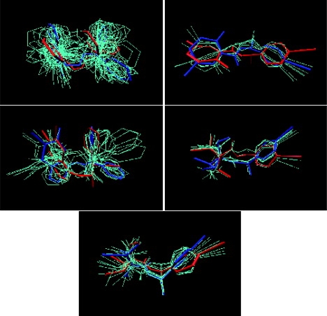
Superimposition of conformations for ligands to scytalone dehydratase. The blue conformer is the most favorable in the free state (that is, the reference conformer for the well with the largest calculated configuration integral). The red conformer is that of the ligand in the bound state, from the crystal structure. The remaining cyan structures are other suboptimal low-energy conformers in the free state. Only heavy atoms are displayed. The five ligands shown are (3-aminomethyl-cinnolin-4-YL)-(3,3-diphenyl-allylidene)-amine (PDB code 3std), N-[1-(4-bromophenyl)ethyl]-5-fluoro salicylamide (PDB code 4std), 6,7-difluoro-quinazolin-4-YL)-(1-metyl-2,2-diphenyl-ethyl)-amide (PDB code 5std), 2,2-difluoro-1-methanesulfinyl-3-methyl-cyclopropanecarboxylic acid [1-(4-bromo-phenyl)-ethyl]-amide (PDBcode 6 std), and (1RS,3SR)-2,2-dichloro-N-[(R)-1-(4-chlorophenyl)ethyl]-1-ethyl-3-methylcyclopropanecarboxamid (PDB code 7std).

Range of binding affinities

In most subsets, the range of computed binding affinities is much larger than experimental values. Here for five subsets where we obtained strong correlation between computed and experimental binding affinities (R_p > 0.7), we analyzed the standard deviation of experimental and calculated binding affinities. In addition, the calculated binding affinities were decomposed into two terms: the ligand-receptor interaction energy, and the ligand conformational free energy change. The standard deviations of these two terms were also computed. Results are shown in Table S5. In all five subsets, the standard deviations of the two terms are comparable in magnitude to the standard deviation of the calculated binding free energies. Generally, the standard deviation of the ligand-receptor interaction term is larger than the ligand conformational free energy term. However, the standard deviations of these three terms are significantly larger than experimental values, which are normally close to 1 kcal/mol. This unrealistic free energy range has been observed in several previous publications (8,9,29). It was suspected that this overestimation of binding affinities resulted from neglecting or inaccurately computing ligand configurational entropies. For three of five subsets we evaluated, taking into account the ligand energetic and entropic term tends to reduce the range of computed affinities. However, this penalty term is not large enough to compensate for the receptor-ligand interaction term. This suggests that the large range of calculated affinities is due to other factors; one possibility is the inaccurate treatment of the receptor conformational change due to binding. In our calculations, the receptor was restrained to the bound state; therefore, the contribution resulting from the receptor assuming different conformations when bound to different ligands was neglected. We attempted to include the receptor energy term directly in our bound-state QH/FEP calculation. However, this treatment is crude and the noise due to including this term is so large that it dominates the entire free-energy estimate. On the other hand, a previous free energy calculation yields a computed free energy of binding that is in good agreement with experimental value for a set of structurally similar ligands (69). In a later simulation, a set of ligand hits and decoys with lesser structure similarities were investigated (70). The magnitude of energy range is slightly larger, but still reasonable. In both of these calculations, the initial receptor structure is identical for different ligands. When bound to different but structurally similar ligands, the receptor deformation term was therefore small.

Ligand conformational free energy change on binding

As described above, a ligand conformational free energy change on binding was defined as follows:

$$\Delta G_{\text{conf}}\equiv -RT\ln \frac{Z_{\mathrm{L},\text{bound}}}{Z_{\mathrm{L},\text{free}}}$$ (17)

where Z_L,bound is the configuration integral for the ligand in the bound-state well (calculated without including interactions with the protein). Here the solvation energy term of the ligand was recomputed without the presence of binding pocket, as if the ligand were fully solvated in water. Z_L,free is the total configuration integral for the ligand in the free state, which is the sum of integrals for all wells. By construction, ΔG_conf is always positive. Fig. 2 shows a histogram of this quantity for all ligands with at least a thousand structure snapshots in the bound-state well (33 ligands were excluded by this criterion). Calculated values were as large as 33.2 kcal/mol, with an average of 5.77 kcal/mol. For 68% of the ligands examined, ΔG_conf was at least 1 kcal/mol.

Figure 2.

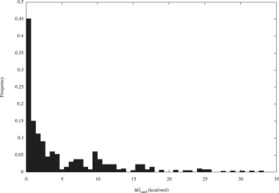
Histogram of the ligand conformational free energy change on binding, ΔG_conf (kcal/mol), for 233 ligands.

The conformational free energy change on binding can be decomposed into enthalpic and entropic contributions:

$$\Delta G_{\text{conf}}\equiv \Delta H_{\text{conf}}-T\Delta S_{\text{conf}}\text{.}$$ (18)

Here ΔH_conf is the difference of the average of the potential for the bound-state well and the free state:

$$\Delta H_{\text{conf}}\equiv \Delta H_{\mathrm{L},\text{bound}}-H_{\mathrm{L},\text{free}},$$ (19)

where

$$H_{\mathrm{L},\text{bound}}={\langle U\rangle }_{\mathrm{L},\text{bound}},$$ (20)

and

$$H_{\mathrm{L},\text{free}}=\frac{{\sum }_{\text{i}}{\langle U_{\mathrm{L}}\rangle }_{\text{i}}{Z}_{\text{i}}}{{\sum }_{\text{i}}{Z}_{\text{i}}},$$ (21)

are averages of the potential over the bound-state well, and over all wells weighted by their configuration integrals, respectively.

The entropic contribution to ΔG_conf is significant, because there is little correlation between ΔG_conf and ΔH_conf (data not shown). Fig. S4 shows that there is a weak, but non-negligible, correlation between −TΔS_conf and the number of rotatable bonds in the ligand. Molecules with fewer rotatable bonds tend to have a smaller conformational entropy change on binding, whereas larger, more flexible molecules have greater configurational entropy changes. The line of best fit gives a slope of 0.47 kcal/mol per rotatable bond at 300 K. This value is within the range of constants used in empirical scoring functions, which is 0.4 to 1.0 kcal/mol per rotatable bond (8). However, the weak correlation suggests that this correction is rather crude. The results are also in agreement with a recent argument (11) that configurational entropy loss on binding is not due primarily to a reduction of the number of accessible rotamers, but to a narrowing of the conformational bound-state well.

Solvation free energy

We also investigated the contribution of differing solvation free energies to relative binding affinities. The solvation free energy may be calculated from the Zwanzig formula:

$$\Delta G_{\text{solv}}=RT\ln {\langle e^{-\left({\text{U}}_{\text{vacuum}}-{\text{U}}_{\text{solution}}\right)/\text{RT}}\rangle }_{\text{solution}}\text{.}$$ (22)

Here U denotes the potential either including or excluding the contribution due to the implicit solvent model, and the average is computed over all wells by weighting each by its configuration integral, as for H_free above. Solvation free energies were calculated for all ligands and compared with values for ΔG_bind. Although differences in ΔG_solv were comparable in magnitude to differences in ΔG_bind for each protein subset, for most subsets, there was almost no correlation between the two quantities (data not shown).

Conclusions

We examined a method for calculating configuration integrals based on perturbation theory using a quasi-harmonic reference system. A reference conformation is chosen and a relatively short simulation is run to generate a covariance matrix. This is used to construct a harmonic system, whose configuration integral can be calculated analytically. The integral for the actual system can then be evaluated using perturbation theory, with the QH model used as a reference. The method is applicable to calculations in Cartesian or bond-angle-torsion coordinates. For the latter, we calculated a correction due to the Jacobian factor arising from the coordinate transformation. We tested the accuracy of the method by numerical calculations on small model systems. For several of the test systems, the QH approximation by itself does not give accurate results, but including the FEP correction results in good agreement with the exact value for systems for which it can be calculated analytically. We also compared excess free energy differences calculated by QH/FEP with those from standard FEP between states; the two methods give values in close agreement. The method may be extended to multiple reference systems by choosing several low-energy reference conformations, defining a well for each to consist of all geometries closer to that reference conformation than any other, evaluating configuration integrals for each well separately, and adding integrals to obtain a total for the entire system.

We used this method to examine the free energy change due to ligand conformational restriction on binding. Binding affinities for protein-ligand complexes taken from the refined set of the PDBbind database were calculated, using the generalized AMBER force field with the GBSA implicit solvent model. Including the contribution due to ligand conformational restriction improves the agreement between calculated and measured affinities. For most ligands, there is a significant difference between the bound-state conformation and the most favorable conformation in the free state. The ligand conformational free energy change on binding, as given by the ratio of configuration integrals computed for the bound and free states, is a significant contributor to binding affinity, and is due to entropic as well as enthalpic contributions.

Supporting Material

Four figures and five tables are available at http://www.biophysj.org/biophysj/supplemental/S0006-3495(09)01746-9.

References

- 1.Vaque M., Ardrevol A., Pujadas G. Protein-ligand docking: a review of recent advances and future perspectives. Curr. Pharm. Anal. 2008;4:1–19. [Google Scholar]
- 2.Warren G.L., Andrews C.W., Head M.S. A critical assessment of docking programs and scoring functions. J. Med. Chem. 2006;49:5912–5931. doi: 10.1021/jm050362n. [DOI] [PubMed] [Google Scholar]
- 3.Kim R., Skolnick J. Assessment of programs for ligand binding affinity prediction. J. Comput. Chem. 2008;29:1316–1331. doi: 10.1002/jcc.20893. [DOI] [PMC free article] [PubMed] [Google Scholar]
- 4.Perola E., Charifson P.S. Conformational analysis of drug-like molecules bound to proteins: an extensive study of ligand reorganization upon binding. J. Med. Chem. 2004;47:2499–2510. doi: 10.1021/jm030563w. [DOI] [PubMed] [Google Scholar]
- 5.Tirado-Rives J., Jorgensen W.L. Contribution of conformer focusing to the uncertainty in predicting free energies for protein-ligand binding. J. Med. Chem. 2006;49:5880–5884. doi: 10.1021/jm060763i. [DOI] [PubMed] [Google Scholar]
- 6.Pickett S.D., Sternberg M.J. Empirical scale of side-chain conformational entropy in protein folding. J. Mol. Biol. 1993;231:825–839. doi: 10.1006/jmbi.1993.1329. [DOI] [PubMed] [Google Scholar]
- 7.Raha K., Merz K.M. Large-scale validation of a quantum mechanics based scoring function: predicting the binding affinity and the binding mode of a diverse set of protein-ligand complexes. J. Med. Chem. 2005;48:4558–4575. doi: 10.1021/jm048973n. [DOI] [PubMed] [Google Scholar]
- 8.Gilson M.K., Zhou H.-X. Calculation of protein-ligand binding affinities. Annu. Rev. Biophys. Biomol. Struct. 2007;36:21–42. doi: 10.1146/annurev.biophys.36.040306.132550. [DOI] [PubMed] [Google Scholar]
- 9.Chen W., Chang C.-E., Gilson M.K. Calculation of cyclodextrin binding affinities: energy, entropy, and implications for drug design. Biophys. J. 2004;87:3035–3049. doi: 10.1529/biophysj.104.049494. [DOI] [PMC free article] [PubMed] [Google Scholar]
- 10.Chang C.-E., Gilson M.K. Free energy, entropy, and induced fit in host-guest recognition: calculations with the second-generation mining minima algorithm. J. Am. Chem. Soc. 2004;126:13156–13164. doi: 10.1021/ja047115d. [DOI] [PubMed] [Google Scholar]
- 11.Chang C.-E., Chen W., Gilson M.K. Ligand configurational entropy and protein binding. Proc. Natl. Acad. Sci. USA. 2007;104:1534–1539. doi: 10.1073/pnas.0610494104. [DOI] [PMC free article] [PubMed] [Google Scholar]
- 12.Jorgensen W.L. Free energy calculations: a breakthrough for modeling organic chemistry in solution. Acc. Chem. Res. 1989;22:184–189. [Google Scholar]
- 13.Kollman P. Free energy calculations: applications to chemical and biochemical phenomena. Chem. Rev. 1993;93:2395–2417. [Google Scholar]
- 14.Gilson M.K., Given J.A., McCammon J.A. The statistical-thermodynamic basis for computation of binding affinities: a critical review. Biophys. J. 1997;72:1047–1069. doi: 10.1016/S0006-3495(97)78756-3. [DOI] [PMC free article] [PubMed] [Google Scholar]
- 15.Boresch S., Tettinger F., Karplus M. Absolute binding free energies: a quantitative approach for their calculation. J. Phys. Chem. B. 2003;107:9535–9551. [Google Scholar]
- 16.Tembe B.L., McCammon J.A. Ligand receptor interactions. Comput. Chem. 1984;8:281–283. [Google Scholar]
- 17.Deng Y., Roux B. Calculation of standard binding free energies: aromatic molecules in the T4 lysozyme L99A mutant. J. Chem. Theory Comput. 2006;2:1255–1273. doi: 10.1021/ct060037v. [DOI] [PubMed] [Google Scholar]
- 18.Wang J., Deng Y., Roux B. Absolute binding free energy calculations using molecular dynamics simulations with restraining potentials. Biophys. J. 2006;91:2798–2814. doi: 10.1529/biophysj.106.084301. [DOI] [PMC free article] [PubMed] [Google Scholar]
- 19.Mobley D.L., Chodera J.D., Dill K.A. On the use of orientational restraints and symmetry corrections in alchemical free energy calculations. J. Chem. Phys. 2006;125:084902. doi: 10.1063/1.2221683. [DOI] [PMC free article] [PubMed] [Google Scholar]
- 20.Woo H.-J., Roux B. Calculation of absolute protein-ligand binding free energy from computer simulations. Proc. Natl. Acad. Sci. USA. 2005;102:6825–6830. doi: 10.1073/pnas.0409005102. [DOI] [PMC free article] [PubMed] [Google Scholar]
- 21.Gan W., Roux B. Binding specificity of SH2 domains: insight from free energy simulations. Proteins. 2008;74:996–1007. doi: 10.1002/prot.22209. [DOI] [PMC free article] [PubMed] [Google Scholar]
- 22.Shirts M.R., Pitera J.W., Pande V.S. Extremely precise free energy calculations of amino acid side chain analogs: comparison of common molecular mechanics force fields for proteins. J. Chem. Phys. 2003;119:5740. [Google Scholar]
- 23.Fujitani H., Tanida Y., Pande V.S. Direct calculation of the binding free energies of FKBP ligands. J. Chem. Phys. 2005;123:084108. doi: 10.1063/1.1999637. [DOI] [PubMed] [Google Scholar]
- 24.Deng Y., Roux B. Computations of standard binding free energies with molecular dynamics simulations. J. Phys. Chem. B. 2009;113:2234–2246. doi: 10.1021/jp807701h. [DOI] [PMC free article] [PubMed] [Google Scholar]
- 25.Mobley D.L., Dill K.A. Binding of small-molecule ligands to proteins: “what you see” is not always “what you get”. Structure. 2009;17:489–498. doi: 10.1016/j.str.2009.02.010. [DOI] [PMC free article] [PubMed] [Google Scholar]
- 26.Aqvist J., Medina C., Samuelsson J.E. A new method for predicting binding affinity in computer-aided drug design. Protein Eng. 1994;7:385–391. doi: 10.1093/protein/7.3.385. [DOI] [PubMed] [Google Scholar]
- 27.Zhou R.H., Friesner R.A., Levy R.M. New linear interaction method for binding affinity calculations using a continuum solvent model. J. Phys. Chem. B. 2001;105:10388–10397. [Google Scholar]
- 28.Kollman P.A., Massova I., Cheatham T.E. Calculating structures and free energies of complex molecules: combining molecular mechanics and continuum models. Acc. Chem. Res. 2000;33:889–897. doi: 10.1021/ar000033j. [DOI] [PubMed] [Google Scholar]
- 29.Brown S.P., Muchmore S.W. High-throughput calculation of protein-ligand binding affinities: modification and adaptation of the MM-PBSA protocol to enterprise grid computing. J. Chem. Inf. Model. 2006;46:999–1005. doi: 10.1021/ci050488t. [DOI] [PubMed] [Google Scholar]
- 30.Mobley D.L., Dill K.A., Chodera J.D. Treating entropy and conformational changes in implicit solvent simulations of small molecules. J. Phys. Chem. B. 2008;112:938–946. doi: 10.1021/jp0764384. [DOI] [PMC free article] [PubMed] [Google Scholar]
- 31.Karplus M., Kushick J.N. Method for estimating the configurational entropy of macromolecules. Macromolecules. 1981;14:325–332. [Google Scholar]
- 32.Brooks B.R., Janežič D., Karplus M. Harmonic analysis of large systems. 1. Methodology. J. Comput. Chem. 1995;16:1522–1542. [Google Scholar]
- 33.Janežič D., Brooks B.R. Harmonic analysis of large systems. 2. Comparison of different protein models. J. Comput. Chem. 1995;16:1543–1553. [Google Scholar]
- 34.Janežič D., Venable R.M., Brooks B.R. Harmonic analysis of large systems. 3. Comparison with molecular dynamics. J. Comput. Chem. 1995;16:1554–1566. [Google Scholar]
- 35.Cecchini M., Krivov S.V., Karplus M. Calculation of free-energy differences by confinement simulations. Application to peptide conformers. J. Phys. Chem. B. 2009;113:9728–9740. doi: 10.1021/jp9020646. [DOI] [PMC free article] [PubMed] [Google Scholar]
- 36.Chang C.-E., Chen W., Gilson M.K. Evaluating the accuracy of the quasi-harmonic approximation. J. Chem. Theory Comput. 2005;1:1017–1028. doi: 10.1021/ct0500904. [DOI] [PubMed] [Google Scholar]
- 37.Huang L., Makarov D.E. On the calculation of absolute free energies from molecular-dynamics or Monte Carlo data. J. Chem. Phys. 2006;124:064108. doi: 10.1063/1.2166397. [DOI] [PubMed] [Google Scholar]
- 38.Frenkel D., Ladd A.J.C. New Monte Carlo method to compute the free energy of arbitrary solids—application to the FCC and HCP phases of hard spheres. J. Chem. Phys. 1984;81:3188–3193. [Google Scholar]
- 39.Stoessel J.P., Nowak P. Absolute free energies in biomolecular systems. Macromolecules. 1990;23:1961–1965. [Google Scholar]
- 40.Levesque D., Verlet L. Perturbation theory and equation of state for fluids. Phys. Rev. 1969;182:307. [Google Scholar]
- 41.Tyka M.D., Sessions R.B., Clarke A.R. Absolute free-energy calculations of liquids using a harmonic reference state. J. Phys. Chem. B. 2007;111:9571–9580. doi: 10.1021/jp072357w. [DOI] [PubMed] [Google Scholar]
- 42.Roux B., Nina M., Smith J.C. Thermodynamic stability of water molecules in the bacteriorhodopsin proton channel: a molecular dynamics free energy perturbation study. Biophys. J. 1996;71:670–681. doi: 10.1016/S0006-3495(96)79267-6. [DOI] [PMC free article] [PubMed] [Google Scholar]
- 43.Ytreberg F.M., Zuckerman D.M. Simple estimation of absolute free energies for biomolecules. J. Chem. Phys. 2006;124:104105. doi: 10.1063/1.2174008. [DOI] [PubMed] [Google Scholar]
- 44.Tyka M.D., Clarke A.R., Sessions R.B. An efficient, path-independent method for free-energy calculations. J. Phys. Chem. B. 2006;110:17212–17220. doi: 10.1021/jp060734j. [DOI] [PubMed] [Google Scholar]
- 45.Mobley D.L., Graves A.P., Dill K.A. Predicting absolute ligand binding free energies to a simple model site. J. Mol. Biol. 2007;371:1118–1134. doi: 10.1016/j.jmb.2007.06.002. [DOI] [PMC free article] [PubMed] [Google Scholar]
- 46.Chang C.-E., Potter M., Gilson M. Calculation of molecular configuration integrals. J. Phys. Chem. B. 2003;107:1048–1055. [Google Scholar]
- 47.Kolossvary I. Evaluation of the molecular configuration integral in all degrees of freedom for the direct calculation of conformational free energies: prediction of the anomeric free energy of monosaccharides. J. Phys. Chem. A. 1997;101:9900–9905. [Google Scholar]
- 48.Wang R., Fang X., Wang S. The PDBbind database: collection of binding affinities for protein-ligand complexes with known three-dimensional structures. J. Med. Chem. 2004;47:2977–2980. doi: 10.1021/jm030580l. [DOI] [PubMed] [Google Scholar]
- 49.Wang R., Fang X., Wang S. The PDBbind database: methodologies and updates. J. Med. Chem. 2005;48:4111–4119. doi: 10.1021/jm048957q. [DOI] [PubMed] [Google Scholar]
- 50.Roux B., Simonson T. Implicit solvent models. Biophys. Chem. 1999;78:1–20. doi: 10.1016/s0301-4622(98)00226-9. [DOI] [PubMed] [Google Scholar]
- 51.Zwanzig R. High-temperature equation of state by a perturbation method. I. Nonpolar gases. J. Chem. Phys. 1954;22:1420–1426. [Google Scholar]
- 52.Bennett C.H. Efficient estimation of free-energy differences from Monte Carlo data. J. Comput. Phys. 1976;22:245–268. [Google Scholar]
- 53.Shirts M.R., Bair E., Pande V.S. Equilibrium free energies from nonequilibrium measurements using maximum-likelihood methods. Phys. Rev. Lett. 2003;91:140601. doi: 10.1103/PhysRevLett.91.140601. [DOI] [PubMed] [Google Scholar]
- 54.Potter M.J., Gilson M.K. Coordinate systems and the calculation of molecular properties. J. Phys. Chem. A. 2002;106:563–566. [Google Scholar]
- 55.Pitzer K.S. Energy levels and thermodynamic functions for molecules with internal rotation: II. Unsymmetrical tops attached to a rigid frame. J. Chem. Phys. 1946;14:239. [Google Scholar]
- 56.Brooks B.R., Bruccoleri R.E., Karplus M. CHARMM—a program for macromolecular energy, minimization, and dynamics calculations. J. Comput. Chem. 1983;4:187–217. [Google Scholar]
- 57.Jorgensen W.L., Maxwell D.S., Tirado-Rives J. Development and testing of the OPLS all-atom force field on conformational energetics and properties of organic liquids. J. Am. Chem. Soc. 1996;118:11225. [Google Scholar]
- 58.Wang J., Wolf R.M., Case D.A. Development and testing of a general amber force field. J. Comput. Chem. 2004;25:1157–1174. doi: 10.1002/jcc.20035. [DOI] [PubMed] [Google Scholar]
- 59.Jakalian A., Bush B.L., Bayly C.I. Fast, efficient generation of high-quality atomic charges. AM1-BCC model: I. Method. J. Comput. Chem. 2000;21:132–146. doi: 10.1002/jcc.10128. [DOI] [PubMed] [Google Scholar]
- 60.Qiu D., Shenkin P.S., Still W.C. The GB/SA continuum model for solvation. A fast analytical method for the calculation of approximate Born radii. J. Phys. Chem. A. 1997;101:3005–3014. [Google Scholar]
- 61.Reference deleted in proof.
- 62.Friesner R.A., Banks J.L., Shenkin P.S. Glide: a new approach for rapid, accurate docking and scoring. 1. Method and assessment of docking accuracy. J. Med. Chem. 2004;47:1739–1749. doi: 10.1021/jm0306430. [DOI] [PubMed] [Google Scholar]
- 63.Halgren T.A., Murphy R.B., Banks J.L. Glide: a new approach for rapid, accurate docking and scoring. 2. Enrichment factors in database screening. J. Med. Chem. 2004;47:1750–1759. doi: 10.1021/jm030644s. [DOI] [PubMed] [Google Scholar]
- 64.Ferrara P., Gohlke H., Brooks C.L. Assessing scoring functions for protein-ligand interactions. J. Med. Chem. 2004;47:3032–3047. doi: 10.1021/jm030489h. [DOI] [PubMed] [Google Scholar]
- 65.Velec H.F.G., Gohlke H., Klebe G. DrugScore(CSD)-knowledge-based scoring function derived from small molecule crystal data with superior recognition rate of near-native ligand poses and better affinity prediction. J. Med. Chem. 2005;48:6296–6303. doi: 10.1021/jm050436v. [DOI] [PubMed] [Google Scholar]
- 66.Hensen C., Hermann J.C., Höltje H.D. A combined QM/MM approach to protein—ligand interactions: polarization effects of the HIV-1 protease on selected high affinity inhibitors. J. Med. Chem. 2004;47:6673–6680. doi: 10.1021/jm0497343. [DOI] [PubMed] [Google Scholar]
- 67.Appelt K. Crystal structures of HIV-1 protease-inhibitor complexes. Perspect. Drug Discov. Des. 1993;1:23–48. [Google Scholar]
- 68.Baldwin E.T., Bhat T.N., Erickson J.W. Structure of HIV-1 protease with KNI-272, a tight-binding transition-state analog containing allophenylnorstatine. Structure. 1995;3:581–590. doi: 10.1016/s0969-2126(01)00192-7. [DOI] [PubMed] [Google Scholar]
- 69.Michel J., Verdonk M.L., Essex J.W. Protein-ligand binding affinity predictions by implicit solvent simulations: a tool for lead optimization? J. Med. Chem. 2006;49:7427–7439. doi: 10.1021/jm061021s. [DOI] [PubMed] [Google Scholar]
- 70.Michel J., Essex J.W. Hit identification and binding mode predictions by rigorous free energy simulations. J. Med. Chem. 2008;51:6654–6664. doi: 10.1021/jm800524s. (r) [DOI] [PubMed] [Google Scholar]
Associated Data
This section collects any data citations, data availability statements, or supplementary materials included in this article.