Reconsidering the asymptotic null distribution of likelihood ratio tests for genetic linkage in multivariate variance components models under complete pleiotropy

Abstract

Accurate knowledge of the null distribution of hypothesis tests is important for valid application of the tests. In previous papers and software, the asymptotic null distribution of likelihood ratio tests for detecting genetic linkage in multivariate variance components models has been stated to be a mixture of chi-square distributions with binomial mixing probabilities. For variance components models under the complete pleiotropy assumption, we show by simulation and by theoretical arguments based on the geometry of the parameter space that all aspects of the previously stated asymptotic null distribution are incorrect—both the binomial mixing probabilities and the chi-square components. Correcting the null distribution gives more conservative critical values than previously stated, yielding P values that can easily be 10 times larger. The true mixing probabilities give the highest probability to the case where all variance parameters are estimated positive, and the mixing components show severe departures from chi-square distributions. Thus, the asymptotic null distribution has complex features that raise challenges for the assessment of significance of multivariate linkage findings. We propose a method to generate an asymptotic null distribution that is much faster than other empirical methods such as permutation, enabling us to obtain P values with higher precision more efficiently.

1. INTRODUCTION AND MAIN RESULTS

Variance components methods are widely used for mapping quantitative trait loci (Almasy and Blangero, 1998; Amos, 1994; Goldgar, 1990; Schork, 1993; SOLAR, 2008). Multivariate extensions of variance components methods, which simultaneously test genetic effects on multiple traits by exploiting extra information related to correlations among the traits, have attracted much attention and have been found to be more powerful than univariate methods by several studies (Almasy and others, 1997; Amos and others, 2001; Boomsma and Dolan, 1998; Schmitz and others, 1998; Williams, Begleiter, and others, 1999; Williams, Van Eerdewegh, and others, 1999).

The asymptotic null distribution of a univariate variance components test, which is a likelihood ratio test for comparing the full model to the null model where the genetic effect variance parameter is constrained to zero, is well known to be a 50:50 mixture of a point mass at zero and ${\chi }_1^2$ (the chi-squared distribution with 1 degree of freedom). This nonstandard limiting distribution arises because the parameter of interest lies on the boundary of the parameter space under the null hypothesis (Self and Liang, 1987).

An analogous mixture distribution was applied to multivariate variance components tests by a number of papers (Almasy and others, 1997; Amos and others, 2001; Amos and de Andrade, 2001; Kraft and others, 2004; Williams, Begleiter, and others, 1999; Williams, Van Eerdewegh, and others, 1999) in which the asymptotic null distribution of the tests was stated to be a mixture of a point mass at zero and several chi-squared distributions, with binomial mixing probabilities. This multivariate method has become widely available; for example, it is implemented in SOLAR (Almasy and Blangero, 1998; SOLAR, 2008), one of the most commonly used software packages for mapping quantitative loci.

However, the evaluation and verification of the asymptotic null distribution of this test have not yet been done systematically. As part of a study comparing the power of univariate to bivariate variance components methods, Amos and others (2001) conducted a simulation of the null distribution. Their bivariate simulation result was not consistent with the previously stated asymptotic null distribution that they assumed, but the source and nature of the inconsistency have remained unexplained (Amos and de Andrade, 2001).

Here we study the null distribution of multivariate variance components tests under a complete pleiotropy assumption. We demonstrate that all aspects of the previously stated asymptotic null distribution are incorrect—both the binomial mixing probabilities and the chi-squared components. We propose a method to assess pointwise significance by generating the asymptotic null distribution making use of the Fisher information estimated from given data. In an example application to an illustrative data set, we compare our method to other well-known empirical methods such as gene-dropping, permutation, and bootstrap methods.

2. BACKGROUND

2.1. Variance components linkage methods

Variance components linkage methods partition the variance of the traits into several random-effect components, one of which captures the influence of a hypothesized “major gene” that affects the traits. In univariate models, the response variable includes a single measured trait for each individual, modeled as a sum of 3 independent normally distributed random effects: an additive major gene effect, which is to be tested on each genetic marker, a polygenic effect, and an environmental effect with corresponding variance parameters $a^2$, $g^2$, and $e^2$, respectively. For simplicity, here let us assume one sib-pair in each family. The trait vector for the ith family follows a multivariate normal distribution: $y_i=(y_{i1,}{y}_{i2})\sim N(\mu ,{\Sigma }_i)$ with

Here the identity by descent (IBD) sharing proportion ${\pi }_{i,12}$ quantifies the allele sharing between individuals 1 and 2 at the locus being tested. The kinship coefficient ${\varphi }_{i,12}$ between individuals 1 and 2 is obtained from the pedigree without using any genetic marker information; for example, for a sib-pair, ϕ_{i, 12} = . Linkage is tested by comparing the null hypothesis $H_0:a^2=0$ to the alternative $H_1:a^2>0$. The likelihood ratio test (LRT) statistic is twice the difference between the log-likelihood of the full model and the model restricted according to the null hypothesis. The parameter $a^2$, which must be nonnegative, lies on the boundary of the parameter space under the null hypothesis $a^2=0$, so that a nonstandard boundary condition applies (Self and Liang, 1987), and the asymptotic null distribution of LRT is χ₀² + χ₁², that is, the mixture distribution of 50% point mass at zero (equivalent to ${\chi }_0^2$) and 50 % ${\chi }_1^2$.

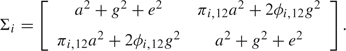
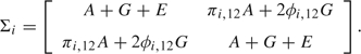
Multivariate variance components models are a natural extension of the above single-trait model, where the response variables include k measured traits for each individual. Continuing to illustrate with the case of one sib-pair per family, $y_i=(y_{i11,}{y}_{i12},\dots ,y_{i1k};y_{i21,}{y}_{i22},\dots ,y_{i2k})\sim N(\mu ,{\Sigma }_i)$, where $y_{ijt}$ is the value of trait t measured on individual j in family i and

(2.1)

Here $G=(g_{ij})$ and $E=(e_{ij})$ are general $k\times k$ covariance matrices for the polygenic effect and environmental effect, respectively. The covariance matrix for the additive major gene effect, $A(a_{ij})$, is assumed to be an outer product of the form $A=(a_1{a}_2\cdots a_k{)}^T(a_1{a}_2\cdots a_k)$. Here the variances, which are the diagonal entries $a_1^2,\dots ,a_k^2$, are of course nonnegative, but the entries $a_1$ can take both positive and negative values, so that the covariances $a_{ij}=a_i{a}_j$ can be positive or negative. The null hypothesis to be tested, $H_0:a_1^2=\cdots =a_k^2=0$, is that all the major gene effect variances are 0. The parameters in the matrices G and E are nuisance parameters.

This model, also known as the “single-factor model” (Evans and others, 2004; Vogler and others, 1997) or the “complete pleiotropic model” (Almasy and others, 1997; Amos and others, 2001; Amos and de Andrade, 2001; Kraft and others, 2004; Williams, Begleiter, and others, 1999; Williams, Van Eerdewegh, and others, 1999), arises when the dominance components of variance for the effects of a single major gene on each trait are assumed to be 0. The idea of the assumed form for A is that the effect on a given trait of a given major gene genotype is a proportionality constant that depends on the trait times an effect size that depends on the genotype. That is, the major gene genotype is modeled as a latent factor that affects the traits in a linear pleiotropic manner. The single-factor model has been extensively used (Amos and others, 2001; Amos and de Andrade, 2001; Evans, 2002; Evans and Duffy, 2004; Evans and others, 2004; Marlow and others, 2003; Monaco, 2007; Vogler and others, 1997). Later, we will use the term “general model” for models without the complete pleiotropic constraint.

2.2. Asymptotic null distributions and binomial mixing probabilities

The null hypothesis of the LRT in the models discussed above violates the regularity conditions that imply the typical asymptotic chi-square distribution, the most obvious violation being that constraining a variance to be 0 forces the variance to lie in the boundary of the parameter space rather than its interior. In the previous work (Amos and others, 2001; SOLAR, 2008), the asymptotic null distribution of the multivariate LRT statistic for testing k traits has been stated to be a mixture distribution of point mass at zero and chi-square distributions with degrees of freedom from 1 to k, with mixing probabilities coming from the Binomial distribution B(k, ), that is,

(2.2)

Table 1 shows mixing probabilities and critical values according to formula (2.2) for significance levels $\alpha =0.01$ and 0.05 for k-trait asymptotic null distributions for $k=2,3,4$, and 5.

Table 1.

Mixing probabilities and critical values of the previously stated asymptotic null distributions for k-trait multivariate tests according to the binomial mixture formula (2.2)

	χ02	χ12	χ22	χ32	χ42	χ52	Critical value (α = 0.01)	Critical value (α = 0.05)
k = 2	0.2500	0.5000	0.2500				7.289	4.231
k = 3	0.1250	0.3750	0.3750	0.1250			8.746	5.435
k = 4	0.0625	0.2500	0.3750	0.2500	0.0625		10.019	6.498
k = 5	0.0313	0.1563	0.3125	0.3125	0.1563	0.0313	11.183	7.480

3. SIMULATIONS

3.1. Methods

We simulated the null distributions of k-trait multivariate LRT statistics for $k=2,3,4$, and 5. For each test, we generated 1000 data sets each including 2000 independent sib-pairs with traits simulated under the truth of the null hypothesis $H_0:a_1^2=\cdots =a_k^2=0$ using the multivariate normal distributions specified at (2.1). Each trait had total variance 1 with $g_{11}=\cdots =g_{kk}=0.4$ (i.e. the polygenic effect explained 40% of the total variance of each trait) and $e_{11}=\cdots =e_{kk}=0.6$ (i.e. the rest of the variance was due to environmental effects). Polygenic and environmental correlation coefficients among traits were assigned the value 0.1, so that $g_{ij}=0.04$ and $e_{ij}=0.06$ for $i\ne j$. The IBD sharing levels ${\pi }_{i,12}$ were simulated from {0, 1/2, 1} with probabilities {1/4, 1/2, 1/4}, respectively, which amounts to assuming complete linkage information and random sampling.

Optimization was done using the Mx software (Neale and others, 1999). We recorded the LRT statistic and estimates for each replicate data set. In order to separate the mixture distribution of LRT into its components, we grouped the replicate results by the number of major gene variance parameters that were estimated positive, which we will denote by v. There were $k+1$ groups, starting from 0 (where none of the k parameters was estimated positive) up to k (where all the k parameters were estimated positive), so that v took its values in $\{0,1,2,\dots ,k\}$. The empirical mixing probabilities were calculated simply as the fraction of each group within the total number of replicates.

3.2. Results

Table 2, which shows the results of the null distribution simulations, reveals that the mixing probabilities do not agree with the probabilities anticipated in Table 1, that is, the binomial distribution previously used in the literature and software. For example for $k=2$, the probabilities for v taking the values 0, 1, and 2 are 0.142, 0, and 0.858, respectively, whereas the corresponding binomial probabilities are 0.25, 0.5, and 0.25. The substantial discrepancies already seen in the case $k=2$ become larger for higher k. Instead of a binomial distribution having probabilities for $v=0,1,2,\dots ,k$, the true mixing distribution puts positive probability only on $v=0$ and $v=k$. Furthermore, rather than having equal probabilities for the cases $v=0$ and $v=k$, the true distribution puts larger probability on $v=k$, and this effect becomes more extreme as k increases. Empirical null distributions of LRT statistics for k-trait multivariate tests for the cases where $v=k$. The blue curve is the ${\chi }_k^2$ density.

Table 2.

Mixing probabilities, K-S tests, and critical values for k-trait multivariate test null distributions obtained by simulations. The first 6 columns are probabilities for various values for v, calculated as the fraction of replicates that yielded that value for v. The Kolmogorov tests were conducted for the v = k cases

	Number of major gene effect variance parameters estimated positive (v)						K-S test (P value)	Critical value
	0	1	2	3	4	5		α = 0.01	α = 0.05
k = 2	0.142	—	0.858				3.3 × 10−12	8.640	5.485
k = 3	0.020	—	—	0.980			4.4 × 10−9	12.221	7.696
k = 4	0.001	—	—	—	0.999		8.2 × 10−4	14.820	10.172
k = 5	—	—	—	—	—	1.000	2.4 × 10−14	15.693	12.458

Figure 1 shows empirical distributions of the LRT statistics in the cases where $v=k$. We focused on these cases since, as shown in Table 2, only the $v=k$ component had large enough counts to be drawn as histogram. Figure 1 reveals some departures from the anticipated ${\chi }^2$ distributions. In $k=2$ and 3, there are more points near zero than anticipated, in $k=5$, the distribution is shifted to the right compared to the ${\chi }_5^2$ curve, and $k=4$ is somewhat in between these 2 different patterns. To quantify the departure from the anticipated ${\chi }_k^2$ distributions, we conducted Kolmogorov–Smirnov (K-S) tests, and the results are shown in Table 2. From the small P values we conclude that the empirical distributions do not follow the anticipated ${\chi }_k^2$ distributions.

Fig. 1.

Empirical null distributions of LRT statistics for k-trait multivariate tests for the cases where v = k. The blue curve is the χ_k² density.

The last 2 columns in Table 2 are critical values for the significance levels $\alpha =0.01$ and 0.05. Compared to the critical values anticipated in Table 1, these critical values are larger, that is, more conservative. This implies that the previously stated null distribution can lead to false-positive findings. For example, suppose we observe an LRT statistic value 14 in a multivariate test with $k=5$ traits, which the previously stated null distribution assigns a P value of 0.002849. According to the simulated null distribution, however, the true P value is 0.025, which is about 10 times less significant.

4. GEOMETRIC EXPLANATIONS AND APPLICATIONS

Our simulation results contain a number of interesting features: (i) zero mixing proportion for the case where only a subset of boundary parameters are estimated positive and highest proportion on the case where all variance parameters are estimated positive and (ii) departure from chi-square distributions within the mixing components. Here we explain these results using theoretical arguments based on the geometry of the parameter space.

The LRT of the null hypothesis $\theta \in {\Omega }_0$ versus the alternative hypothesis $\theta \in {\Omega }_1$ uses the LRT statistic $2\text{log}({\text{sup}}_{\theta \in {\Omega }_1}L\left(\theta \right))-2\text{log}({\text{sup}}_{\theta \in {\Omega }_0}L\left(\theta \right))$, where L is the likelihood function. According to Theorem 3 in Self and Liang (1987), when $\theta ={\theta }_0$, under certain regularity conditions, the asymptotic distribution of LRT is the same as the distribution of the LRT for testing $\theta \in C_{{\Omega }_0}$ versus $\theta \in C_{{\Omega }_1}$ based on a single observation Y, where $Y\sim N(\theta ,I^{-1}({\theta }_0\left)\right)$ and $C_{{\Omega }_0}$ and $C_{{\Omega }_1}$ are cones approximating ${\Omega }_0$ and ${\Omega }_1$ at ${\theta }_0$. This latter LRT takes the form ${\text{inf}}_{\theta \in C_{{\Omega }_0}}(Y-\theta {)}^{T}I\left({\theta }_0\right)\left(Y-\theta \right)-{\text{inf}}_{\theta \in C_{{\Omega }_1}}(Y-\theta {)}^{T}I\left({\theta }_0\right)\left(Y-\theta \right),$ so that, defining $Z=Y-{\theta }_0$, the LRT is equivalent to

(4.1)

where $C_{{\Omega }_0}-{\theta }_0=\{\theta -{\theta }_0:\theta \in C_{{\Omega }_0}\}$ and $Z\sim N(0,I^{-1}({\theta }_0\left)\right)$ under the null hypothesis. For the special case when $I({\theta }_0)$ is the identity matrix I,

(4.2)

So in the case $I({\theta }_0)=I$, LRT is the difference between the squared (Euclidean) distance from Z to $C_{{\Omega }_0}-{\theta }_0$ and squared distance from Z to $C_{{\Omega }_1}-{\theta }_0$.

Below, we will mainly write expressions explicitly for the case of $k=2$ traits with the information matrix $I({\theta }_0)$ being the identity matrix, which reveals the essential ideas with minimal notational complexity.

4.1. Mixing probabilities

A way of thinking about the problem that is tempting but leads to incorrect conclusions, including the asymptotic distribution incorrectly stated in previous papers, is as follows. Denote the parameters of interest by $\theta =({\theta }_1,{\theta }_2)=(a_{11},a_{22})=(a_1^2,a_2^2)$. The null hypothesis ${\Omega }_0$ is $\theta =(0,0)$, and the alternative ${\Omega }_1$ is the first quadrant $\theta \in \left\{\right({\theta }_1,{\theta }_2):{\theta }_1>0,{\theta }_2>0\}$, and the approximating cones $C_{{\Omega }_0}$ and $C_{{\Omega }_1}$ are the same as ${\Omega }_0$ and ${\Omega }_1$. Let $Z\sim N(0,I)$ and where is the vector θ that achieves the infimum in ${\text{inf}}_{\theta \in {\Omega }_1}\Vert Z-\theta {\Vert }^2$, that is, the projection of Z onto the first quadrant ${\Omega }_1$. The random point $Z=(Z_1,Z_2)$ falls in each of the 4 quadrants (regions in Figure 2) with equal probability $1/4$. When Z falls in the first quadrant (region , probability 1/4), $\text{LRT}=\Vert Z{\Vert }^2$ (because is simply Z itself, so that ‖Z − ‖² = 0), which is distributed as ${\chi }_2^2$, and both ₁ and ₂ are positive. When Z lies in the second quadrant, (₁, ₂) = (0, Z₂), so that $\text{LRT}=\Vert Z{\Vert }^2-Z_1^2=Z_2^2\sim {\chi }_1^2$, and only ${\theta }_2$ is estimated positive. Symmetric logic applies to the fourth quadrant, so that $\text{LRT}=Z_1^2\sim {\chi }_1^2$, and only ${\theta }_1$ is estimated positive. When Z lies in the third quadrant, the projection (₁, ) = (0, 0), so that $\text{LRT}=\Vert Z{\Vert }^2-\Vert Z{\Vert }^2=0$ and both parameters are estimated zero. In summary, LRT is distributed as the mixture 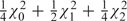, with the different mixture components determined by the number of parameters estimated positive.

Fig. 2.

The parameter space θ ∈ {(θ₁, θ₂): θ₁ > 0, θ₂ > 0}.

The above reasoning, however, ignores the covariance parameter $a_{12}$. For simplicity, let us focus our attention on the parameters of interest $a_{11},a_{22}$, and $a_{12}$ and ignore the nuisance parameters in the model that describe the polygenic and environmental effects. The single-factor model is constrained according to $a_{12}=a_1{a}_2$. That is, letting $\theta =({\theta }_1,{\theta }_2,{\theta }_3)=(a_{11},a_{22},a_{12})=(a_1^2,a_2^2,a_1{a}_2)$, the constraint in the single-factor model is expressed by . So for this problem, the null hypothesis is ${\Omega }_0=\{\theta \in {ℝ}^3:({\theta }_1,{\theta }_2,{\theta }_3)=(0,0,0\left)\right\}$ and the alternative hypothesis is . Here we are thinking of the parameter space as a curved surface in 3-dimensional space, not just a single quadrant in the 2-dimensional space $\left\{\right(a_{11},a_{22}\left)\right\}$. Figures 3(a) and (b) show this surface from different angles. To apply Theorem 3 of Self and Liang (1987) to this problem, we note that the hypotheses ${\Omega }_0=\{\theta =(0,0,0)\}$ and ${\Omega }_1$ are already cones, so that the approximating cones are $C_{{\Omega }_0}={\Omega }_0$ and $C_{{\Omega }_1}={\Omega }_1$. Suppose for illustration that the information matrix under the null hypothesis, $I(0,0,0)$, is the identity matrix $I=I_3$. A general case will be discussed in Section 4.3.

Fig. 3.

Plots (a) and (b) are the parameter space of points θ = (θ₁, θ₂, θ₃) such that . Plot (c) shows the boundary of the polar cone of the parameter space in blue. Plot (d) shows the points Z that give small LRT values (? 0.02) in green. Plot (e) shows the points z giving v = 0 when z ∼ N(0, I). Plot (f) shows the points Z with v = 0 when the covariance of Z is not the identity matrix, but a general covariance matrix obtained from the Fisher information matrix of a genetic model.

The above problem arises from the original genetic problem by using its asymptotic equivalence to a problem with a single observation from a Gaussian distribution, ignoring nuisance parameters, and considering the special case where the information matrix is the identity. Assume the null hypothesis holds. As in (4.2), the asymptotic distribution of the LRT is the same as the distribution of , where $Z\sim N(0,I)$ and = (₁, ₂, ₃) is the vector θ that achieves the infimum in ${\text{inf}}_{\theta \in {\Omega }_1}\Vert Z-\theta {\Vert }^2$, that is, the projection of Z onto the alternative hypothesis surface ${\Omega }_1$

The distribution of LRT is a mixture of components that are distinguished by the number of variance parameters ₁ and ₂ that are estimated positive (which, by the constraint that defines ${\Omega }_1$, also determines whether or not ₃ is estimated nonzero). As before, let v be the number of variance parameters ₁ and ₂ that are estimated positive, that is, the number of positive components among ₁ and ₂; the possible values for v are 0, 1, and 2.

The determination of v can be explained using the polar cone of the parameter space ${\Omega }_1$. The polar cone of ${\Omega }_1$ is defined to be the set $P_{{\Omega }_1}=\{Z\in {ℝ}^3:Z·\theta \le 0\forall \theta \in {\Omega }_1\}$. Figure 3(c) depicts the boundary of the polar cone of the parameter space.

When Z is in the polar cone, we claim $v=0$. To see this, assume $Z\in P_{{\Omega }_1}$ and note that if $\theta \in {\Omega }_1$, then $Z·\theta \le 0$ by definition of the polar cone, which implies $\Vert Z-0{\Vert }^2\le \Vert Z-\theta {\Vert }^2$. Thus, the origin is the point in ${\Omega }_1$ that is closest to Z, which gives $v=0$.

When Z lies outside the polar cone, we claim $v=2$ with probability 1. First, by definition, for any point Z outside the polar cone $P_{{\Omega }_1}$, there exists a vector in ${\Omega }_1$ that has positive inner product with Z. This implies that the projection of Z onto that vector is closer to Z than the origin is, proving $v\ne 0$. Second, we want to show $v\ne 1$ with probability 1. Note that $v=1$ can occur when Z lies on the $Z_3=0$ plane in the first, second, and fourth quadrants, which has probability 0. We claim that whenever $Z_3$ is nonzero (which occurs with probability 1), v cannot be 1. This is shown in each quadrant in the following paragraphs.

Suppose $(Z_1,Z_2)$ falls in the first quadrant, that is, $Z_1>0$ and $Z_2>0$. Without loss of generality, suppose $Z_3>0$ (an analogous argument will handle the case $Z_3<0)$ and $Z_1>Z_2$. Then the point in ${\Omega }_1$ having $v=1$ that is closest to Z is $(Z_1,0,0)$. However, it is obvious that for sufficiently small $\epsilon >0$, the point , which has $v=2$, is closer to Z than $(Z_1,0,0)$ is, proving that v cannot be 1. Thus, we have shown that when $(Z_1,Z_2)$ falls in the first quadrant, we have $v=2$ with probability 1.

Suppose $(Z_1,Z_2)$ falls in the second quadrant, that is, $Z_1<0$ and $Z_2>0$. Again suppose $Z_3>0$, and observe that the point in ${\Omega }_1$ having $v\le 1$ that is closest to Z is $(0,Z_2,0)$. Define , and define $D(\epsilon )$ to be the squared distance . The derivative approaches $-\infty$ as $\epsilon \downarrow 0$. Therefore, for sufficiently small positive ϵ, we must have $D(\epsilon )<D\left(0\right)$, so that the point $\theta (\epsilon )$ is closer to Z than $\theta \left(0\right)=(0,Z_2,0)$ is, which implies that $v\le 1$ cannot hold. The case where $(Z_1,Z_2)$ lies in the fourth quadrant is analogous to the case of the second quadrant. Thus, for both the cases of the second and fourth quadrants, we have $v=2$ with probability 1.

In summary, when Z lies inside the polar cone, $v=0$, and when Z lies outside the polar cone, $v=2$ with probability 1. To illustrate this, we generated 10 000 vectors Z from the 3-dimensional Gaussian distribution with mean zero and identity covariance matrix. For each Z, we calculated v by estimating with the optimization being performed under the constraints using the program Mx, which applies here because the projection is also the maximum likelihood estimate in this problem. The red points in Figure 3(e) are the points Z having $v=0$, which form the polar cone of the parameter space.

4.2. Departures from chi-squared distributions

In Section 3.2, one of the departures from the anticipated ${\chi }^2$ distributions we observed was an excessive number of LRT values near 0. These small LRT values result from points Z that are located close to the boundary of the polar cone, where the difference between the squared distance from Z to the origin and the squared distance from Z to the parameter space is small. To visualize this, using the same method of generating Z as described in Section 4.1, we simulated 10 000 vectors Z from $N(0,I_3)$, and for each Z we performed the LRT for testing $H_0:\theta =0$ versus $H_1:\theta \ne 0$ with the optimization being performed under the constraints ${\theta }_1\ge 0,{\theta }_2\ge 0$, and . Then we identified the points Z showing small LRT values ($\le 0.02$) and plotted them as green in Figure 3(d). We see that they are located very close to the outer surface of the polar cone.

Another type of departure we observed from the simulation results, particularly in models with larger numbers of traits, was a pattern that the distribution was shifted to the right compared to the anticipated chi-square distribution. This can be explained by the fact that the parameter space consists of 2 surfaces joined at an angle of less than 180${}^{\text{°}}$. The angle between the 2 surfaces (one blue and the other red; see Figures 3(a) and (b)) in our parameter space is 70.54${}^{\text{°}}$ in the direction ${\theta }_1={\theta }_2$. When Z lies between these 2 surfaces, the projection of Z onto the parameter space involves a choice of whether the point is closer to one surface or the other, and the availability of this choice affects the distribution of LRT. An analogous example for illustration in 2 dimensions can help explain this problem simply. Figure 4 shows 2 different cases. In the first, the parameter space is a 1-dimensional straight line, and in the second, the parameter space is 2 lines joined at the origin with an angle less than $180^{\text{°}}$, say, $90^{\text{°}}$. For both hypothesis-testing problems, the null hypothesis is the origin. For the first case, the LRT is exactly $Z_2^2(=(Z_1^2+Z_2^2)-Z_1^2)$ which is distributed as ${\chi }_1^2$. On the other hand, in the second plot, consider the points A and B lying between the 2 lines forming the parameter space. The point A has LRT $=Z_2^2$, while the point B has LRT $=Z_1^2$; the choice of whether LRT is $Z_1^2$ or $Z_2^2$ depends on whether the point is closer to the first line or the second. Thus, in the first quadrant, LRT is max($Z_1^2,Z_2^2$), which in general is larger than, say, $Z_1^2$, which is distributed as ${\chi }_1^2$. Thus, in the first quadrant, LRT does not have a ${\chi }_1^2$ distribution, but rather a distribution that is stochastically larger than ${\chi }_1^2$. Note that if we change the parameter space by decreasing the angle between the lines, the LRT in the region between the lines becomes closer to $Z_1^2+Z_2^2$, which is distributed as ${\chi }_2^2$. Returning to the 3-dimensional problem, as the angle between the surfaces becomes closer to $0^{\text{°}}$, the distribution of LRT in the region between the surfaces would be closer to ${\chi }_3^2$ because the difference between the squared distance from Z to the origin, which is $Z_1^2+Z_2^2+Z_3^2$, and the squared distance from Z to the alternative space, which is close to zero, would be close to $Z_1^2+Z_2^2+Z_3^2$, which is distributed as ${\chi }_3^2$.

Fig. 4.

Influence on LRT of the angle joining the parts of the parameter. The bold lines form the parameter space and the origin is the null hypothesis.

4.3. General case of $I({\theta }_0)\ne I$ and genetic models

General case of $I({\theta }_0)\ne I$.

So far, for simplicity, we have focused on the special case where the Fisher information $I({\theta }_0)$ was the identity matrix I. For the general case when $I({\theta }_0)\ne I$, the results of the Self and Liang theorem stated in (4.1) show that the asymptotic distribution of the LRT can be analyzed as above (involving a difference between the squared distance from Z to the origin and the squared distance from Z to the parameter space), with the Euclidean distance replaced by the more general Mahalanobis distance $\Vert Z-\theta {\Vert }_{ℳ}^2=(Z-\theta {)}^{T}I\left({\theta }_0\right)\left(Z-\theta \right)$. This distance takes into account the covariance of Z, where $Z\sim N(0,I^{-1}({\theta }_0\left)\right)$. For the multivariate normal model, $I({\theta }_0)$ can be obtained from the formula (Searle and others, 1992)

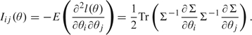(4.3)

Generating the asymptotic null distribution in a genetic model.

The results in (4.1) and (4.3) above allow us to simulate from the asymptotic null distribution in genetic models that have general Fisher information matrices. For example, we did this for the $k=2$ trait genetic model specified in Section 3, that is, the model with parameter values $g_{11}=g_{22}=0.4$, $e_{11}=e_{22}=0.6$, $e_{12}=0.04$ and $e_{12}=0.06$. After obtaining Σ by plugging in the specified values in G and E, using (4.3) we calculated the $9\times 9$ Fisher information matrix for the full set of parameters $(a_{11},a_{22},a_{12};g_{11},g_{22},g_{12};e_{11},g_{22},g_{12})$. After extracting the $3\times 3$ submatrix V of the inverted Fisher information matrix corresponding to the parameters of interest $\theta =(a_{11},a_{22},a_{12})$, we generated 10 000 vectors Z from $N(0,V)$. For each Z, we performed the LRT for testing $H_0:\theta =0$ versus $H_1:\theta \ne 0$ under the constraints ${\theta }_1\ge 0,{\theta }_2\ge 0$, and using Mx. In this application of Mx, we assigned fixed values for the known covariances in V, and Mx optimized the likelihood only over mean parameters. We also determined v using the same technique of comparing a full model to a partially constrained model as described in Section 3.

According to the results, the mixing proportions for $v=0$, $v=1$, and $v=2$ were 0.1477, 0, and 0.8523, and critical values for $\alpha =0.01$ and $\alpha =0.05$ were 8.713 and 5.405, which were quite similar to the results in Table 2. To confirm that the results in this section were consistent with the genetic simulation results for the $k=2$ trait null distribution in Section 3, a K-S test gave a P value of 0.2063.

Plot (f) in Figure 3 shows the points Z with $v=0$ colored as red, filling the polar cone. The contrast between the polar cones in plots (e) and (f) illustrates the effect of having a Fisher information matrix $I({\theta }_0)\ne I$.

Different sets of nuisance parameter values.

To investigate whether and how the asymptotic null distribution is influenced by different choices of the nuisance parameters, we selected 10 sets of nuisance parameters in G and E for each k-trait model, using inverse Wishart distributions to choose matrices that were well spread out over the range of possible covariance matrices. We used the same method described in Section 4.3 to generate the asymptotic null distribution for each set of nuisance parameters. In order to assess whether the asymptotic null distributions generated using different sets of nuisance parameters were different, we conducted pairwise K-S tests. Most of the results did not show significant differences, but the asymptotic distributions for a few of the models were found to have highly significant departures from the rest, showing that the asymptotic distribution does depend on nuisance parameters. For example, Figure 5 shows a case having K-S P value $2.20\times 10^{-16}$.

Fig. 5.

Asymptotic null distributions of tests under 2 models with k = 4 traits.

However, although differences among asymptotic distributions of LRT statistics are real, their practical effect on P values for LRT tests seems to be quite minor. For example, even the pair of asymptotic distributions in Figure 5, which gave the smallest K-S P value we observed, are quite similar. Asymptotic null distributions of tests under 2 models with $k=4$ traits.

5. PROPOSED METHOD FOR GENERATING ASYMPTOTIC NULL DISTRIBUTIONS AND CALCULATING P VALUES

As we have shown, asymptotic null distributions of multivariate linkage tests have several complex features: the mixing probabilities are not binomial distributions and the mixture components show severe departures from chi-square distributions. The asymptotic null distributions also varied depending on nuisance parameter values to some extent. These complexities in the asymptotic null distribution raise challenges for the assessment of significance of multivariate linkage findings. Empirical methods for obtaining P values, including gene-dropping, permutation, and bootstrap methods, involve generating large numbers of replicated data sets, which can require long computation times. Here we propose a method to calculate P values by generating from an asymptotic null distribution. The new method is much faster than other empirical methods and it gives a correct asymptotic distribution. The idea was implicitly used in Section 4.3, although there we assumed knowledge of the nuisance parameter values. Here we specify a method that is applicable to the more realistic situation where we are given data and do not know nuisance parameter values.

The description of the method uses the following notation. In a k-trait model, the total parameter set consists of the parameters in $A=(a_{ij})$, $G=(g_{ij})$, and $E=(e_{ij})$, where each matrix has parameters. The full parameter set contains all $3m$ parameters in A, G, and E. The parameters in A consist of the parameters of interest $\theta =({\theta }_1,{\theta }_2,\dots ,{\theta }_m)$, with constraints of the form ${\theta }_i\ge 0$ for $i\le k$ and for $i>k$, where we write ${\theta }_i=a_{p\left(i\right),q\left(i\right)}$ for $i>k$. For example, for the models with $k=3$ traits, the parameters of interest are $\theta =({\theta }_1,{\theta }_2,{\theta }_3,{\theta }_4,{\theta }_5,{\theta }_6)=(a_{11},a_{22},a_{33},a_{12},a_{13},a_{23})=(a_1^2,a_2^2,a_3^2;a_1{a}_2,a_1{a}_3,a_2{a}_3)$, and the constraints are , and .

5.1. Method

Suppose we have a given data set and have calculated an LRT statistic for a multivariate linkage test for that data set, and we wish to calculate a P value.

STEP 1: Estimate the Fisher information from the given data.

STEP 1(a): Under the null hypothesis, estimate all parameters in the model— and . Use these to form the estimate .

STEP 1(b): Using and the formula (4.3), calculate the $\left(3m\right)\times \left(3m\right)$ Fisher information matrix for the full parameter set and invert it.

STEP 1(c): Extract the $m\times m$ submatrix of the inverted Fisher information matrix corresponding to, the parameters of interest, and denote it as V.

STEP 2: Generate N random vectors Z from the multivariate Normal distribution $N(0,V)$. An appropriate choice of N depends on the desired precision level.

STEP 3: For each Z, perform the LRT for the null hypothesis $H_0:\theta =0$ in the model $Z\sim N(\theta ,V)$, under the constraints ${\theta }_i\ge 0$ for $1\le i\le k$ and for $i>k$. Here the covariance matrix V is fixed at the value calculated in STEP 1(c), and the test is performed by optimizing the likelihood only over the mean parameters in the vector θ.

STEP 4: The P value is calculated as the fraction of LRT values that are larger than or equal to the LRT value calculated from the given data.

An example Mx script that performs the LRT in STEP 3 above is available in the web supplement at http://www.stat.yale.edu/∼sh437/mxExample.

5.2. Applied example in an illustrative data set

In this section, we apply our proposed method and other well-known empirical methods for assessing P values to an illustrative data set and compare the times for completing the tasks. To create the illustrative data set, we simulated 2000 independent sib-pairs with 2 traits generated from the bivariate model with the same parameter values used in Section 3. For each sibling, we simulated a segment of chromosome with length 80 cM, having 16 markers located 5 cM apart. Each marker had 8 equally frequent alleles, and IBD sharing proportions ${\pi }_{i,12}$ were estimated by Merlin (Abecasis and others, 2001) with grid size 2.5 cM. We prespecified a single test point at 22.5 cM on the chromosome where the LRT would be conducted.

We applied 3 well-known methods for obtaining empirical critical values and P values: gene dropping (Terwilliger and others, 1993), permutation (Wan and others, 1997), and the bootstrap (Marlow and others, 2003). Keeping the phenotype data fixed, the gene-dropping method simulates genotypes on founders’ chromosomes using estimated marker allele frequencies and then segregates the chromosomes to offspring using marker recombination fraction information. For the permutation method, we fixed the trait values and permuted IBD estimates among families. The (parametric) bootstrap, which is not as commonly applied in linkage analysis as the previous 2 methods, estimates parameters from a given data set, treats the estimates as if they were true parameters, and generates replicate data sets, keeping the genotypes the same as in the original data. We applied the above 3 methods to our illustrative data set, generating 10 000 replicates for each method using R and running LRTs at the prespecified test point for each replicated data set using Mx. For STEP 2 in our proposed method, we used $N=10000$.

In this experiment, our method took 56 min to complete the task, while the gene-dropping, bootstrap, and permutation methods took 5893, 3182, and 1611 min, respectively (see Table 3). In order to measure the accuracy of the null distribution estimations, we estimated the type 1 error rates for $\alpha =0.01$ and 0.05 based on the critical values shown in Table 2. The results in Table 3 show reasonably accurate performances of all methods in controlling type 1 errors. The K-S tests for comparing these 4 distributions to the reference distribution obtained in Section 3.2 were conducted, and P values were 0.2063, 0.654, 0.2742, and 0.4982 for the proposed method, gene-dropping, bootstrap, and permutation, respectively, none of them showing severe departures.

Table 3.

Comparing the performances of proposed method and 3 empirical methods

Method	Computation time	Type 1 error rates	Type 1 error rates
	(min)	(α = 0.01)	(α = 0.05)
Proposed method	56	0.0107	0.0483
Gene dropping	5893	0.0099	0.0487
Parametric bootstrap	3182	0.0100	0.0451
Permutation	1611	0.0121	0.0547

The empirical methods took longer than our method since they require generating many replicate data sets with each data set including as many observations as in the given data set (2000 in our experiment), whereas our method requires generating only one Gaussian observation in each data set. Also, each Mx optimization took longer for the empirical methods than for our proposed method, again because our proposed method applies Mx to data sets of just one Gaussian observation.

6. DISCUSSION

Evaluating the null distribution of a test statistic is of course a prerequisite for valid P values. The previously stated asymptotic null distribution, which gave strongly anticonservative P values, has been used in several studies. In fact, some researchers (Amos and de Andrade, 2001; Evans and others, 2004; Marlow and others, 2003; Monaco, 2007) have mentioned the possibility that the previously stated asymptotic null distribution might be incorrect. However, clear statements confirming and quantifying these discrepancies and explaining their nature and origin have not appeared previously, and some researchers (Evans and others, 2004; Monaco, 2007) have expressed the desirability of clarifying the asymptotic null distribution of this test. A part of the purpose of this paper is to provide such clarification. Our simulations establish that there is indeed a real problem underlying discrepancies that had been mentioned as a puzzle in these previous papers. A device that enabled our simulations to quantify the discrepancies was to separate the mixture distribution into components defined by the number of variance parameters estimated positive. Our geometric arguments help explain how and why the discrepancies occur and give insight into the true nature of the asymptotic distribution.

It is of interest to understand, for various possible derivations that would falsely lead to the previously stated asymptotic distribution, exactly where the reasoning fails. For the simple case of $k=2$ traits, a belief that the asymptotic null distribution is simply $0.25{\chi }_0^2+0.5{\chi }_1^2+0.25{\chi }_2^2$ would follow from the incorrect reasoning given in Section 4.1. This incorrect reasoning views the parameter space as a quadrant in the 2-dimensional space of possible values for the variance parameters and also makes the further mistake of assuming the information matrix is the identity. Even correcting this reasoning to allow a general information matrix leads only to asymptotic distributions of the form ( − p)χ₀² + χ₁² + pχ₂²; see Case 7 in Self and Liang (1987) for the derivation of this formula. However, this mixture of chi-square distributions is still evidently incorrect, as we have seen that the correct asymptotic distribution has zero mixing probability for the ${\chi }_1^2$ component. All the above reasoning is invalidated by the observation that the parameter space is actually not isomorphic to the first quadrant in 2 dimensions; in fact, for each point $(a_{11},a_{22})$ in the quadrant, there are 2 different points in the parameter space, with one point having a₁₂ = and the other having a₁₂ = −. Since there are 2 distinct distributions for each point in the quadrant, a reasonable attempt to correct this topological problem is to view the parameter space as 2 quadrants. For example, as in Figure 6, we could consider the parameters to be $a_1$ and $a_2$ where $a_1$ can take any real value (including negative numbers) and $a_2$ is constrained to be nonnegative. These 2 parameters determine the covariance $a_{12}$ by the relationship $a_{12}=a_1{a}_2$. More precisely, to make the problem identifiable, we should remove the ray of points $\left\{\right(a_1,a_2):a_1<0,a_2=0\}$ from the parameter space since the 2 points $(a_1,0)$ and $(-a_1,0)$ correspond to the same distribution. Although this modified half-plane gives a correct one-to-one correspondence with the set of distributions in our problem, attempting to apply the reasoning of Self and Liang (1987) to this situation (see their Case 6) would lead to a conjectured asymptotic null distribution of χ₁² + χ₂², which is also incorrect. In fact, the assumptions required for the results of Self and Liang are questionable in our problem in this 2-dimensional formulation since the modified half-plane is not closed and the information matrix at the null hypothesis $(a_1,a_2)=(0,0)$ is the zero matrix. The modified half-plane parameter space.

Fig. 6.

The modified half-plane parameter space.

In this paper, we focused on the model with the complete pleiotropic constraint. This model has been used in many studies instead of the general model that includes additional correlation parameters (Evans, 2002; Evans and Duffy, 2004; Evans and others, 2004; Loo and others, 2004; Marlow and others, 2003; Monaco, 2007; Vogler and others, 1997). One disadvantage of the general model is that optimization is more difficult (Loo and others, 2004). Also, due to the increased number of parameters, the general model has more degrees of freedom than the complete pleiotropic model. A recent study (Han and others, 2009) showed in a related but different context that using the general model is often less powerful than using the complete pleiotropic model due to the increased degrees of freedom.

Although the focus of the current study is on the complete pleiotropic model, our approaches and results can be extended to investigate the general model. The asymptotic null distribution of the LRT in the general model has also been stated to be a mixture of chi-square distributions with binomial mixing probabilities (e.g. Amos and de Andrade, 2001; Amos and others, 2001; SOLAR, 2008). Although the general model does not put explicit constraints on covariance parameters as in the complete pleiotropic model, covariance parameters still have implicit constraints, for example, ensuring that the correlation coefficients lie between $-1$ and 1. For this reason, applying the binomial mixture of chi-square distributions, which does not take the implicit constraints into account, is incorrect. We are currently studying this issue and preparing a separate paper extending the approaches provided by our present study to the general model.

FUNDING

Yale Center for High Performance Computation in Biology and Biomedicine (National Institutes of Health [NIH] grant RR19895-02); NIH (R01 DC007665).

References

- Abecasis GR, Cherny SS, Cookson WO, Cardon LR. Merlin—rapid analysis of dense genetic maps using sparse gene flow trees. Nature Genetics. 2001;30:97–101. doi: 10.1038/ng786. [DOI] [PubMed] [Google Scholar]
- Almasy L, Blangero J. Multipoint quantitative-trait linkage analysis in general pedigrees. American Journal of Human Genetics. 1998;62:1198–1211. doi: 10.1086/301844. [DOI] [PMC free article] [PubMed] [Google Scholar]
- Almasy L, Dyer T, Blangero J. Bivariate quantitative trait linkage analysis: pleiotropy versus co-incident linkages. Genetic Epidemiology. 1997;14:958. doi: 10.1002/(SICI)1098-2272(1997)14:6<953::AID-GEPI65>3.0.CO;2-K. [DOI] [PubMed] [Google Scholar]
- Amos C, de Andrade M, Zhu D. Comparison of multivariate tests for genetic linkage. Human Heredity. 2001;51:133–144. doi: 10.1159/000053334. [DOI] [PubMed] [Google Scholar]
- Amos CI. Robust variance-components approach for assessing genetic linkage in pedigrees. American Journal of Human Genetics. 1994;54:535. [PMC free article] [PubMed] [Google Scholar]
- Amos CI, de Andrade M. Genetic linkage methods for quantitative traits. Statistical Methods in Medical Research. 2001;10:3. doi: 10.1177/096228020101000102. [DOI] [PubMed] [Google Scholar]
- Boomsma DI, Dolan CV. A comparison of power to detect a QTL in sib-pair data using multivariate phenotypes, mean phenotypes, and factor scores. Behavior Genetics. 1998;28:329–340. doi: 10.1023/a:1021665501312. [DOI] [PubMed] [Google Scholar]
- Evans DM. The power of multivariate quantitative-trait loci linkage analysis is influenced by the correlation between variables. The American Journal of Human Genetics. 2002;70:1599–1602. doi: 10.1086/340850. [DOI] [PMC free article] [PubMed] [Google Scholar]
- Evans DM, Duffy DL. A simulation study concerning the effect of varying the residual phenotypic correlation on the power of bivariate quantitative trait loci linkage analysis. Behavior Genetics. 2004;34:135–141. doi: 10.1023/B:BEGE.0000013727.15845.f8. [DOI] [PubMed] [Google Scholar]
- Evans DM, Zhu G, Duffy DL, Montgomery GW, Frazer IH, Martin NG. Multivariate QTL linkage analysis suggests a QTL for platelet count on chromosome 19q. European Journal of Human Genetics. 2004;12:835–842. doi: 10.1038/sj.ejhg.5201248. [DOI] [PubMed] [Google Scholar]
- Goldgar DE. Multipoint analysis of human quantitative genetic variation. American Journal of Human Genetics. 1990;47:957–967. [PMC free article] [PubMed] [Google Scholar]
- Han SS, Grigorenko EL, Chang JT. Uncovering shared common genetic risk factors for various aspects of complex disorders captured in multiple traits. eprint arXiv. 2009;0904.2229 [Google Scholar]
- Kraft P, Bauman L, Yuan JY, Horvath S. Multivariate variance-components analysis of longitudinal blood pressure measurements from the Framingham Heart Study. BMC Genetics. 2004;4:S55. doi: 10.1186/1471-2156-4-S1-S55. [DOI] [PMC free article] [PubMed] [Google Scholar]
- Loo SK, Fisher SE, Francks C, Ogdie MN, MacPhie IL, Yang M, McCracken JT, McGough JJ, Nelson SF, Monaco AP. Genome-wide scan of reading ability in affected sibling pairs with attention-deficit/hyperactivity disorder: unique and shared genetic effects. Molecular Psychiatry. 2004;9:485–493. doi: 10.1038/sj.mp.4001450. [DOI] [PubMed] [Google Scholar]
- Marlow AJ, Fisher SE, Francks C, MacPhie IL, Cherny SS, Richardson AJ, Talcott JB, Stein JF, Monaco AP, Cardon LR. Use of multivariate linkage analysis for dissection of a complex cognitive trait. The American Journal of Human Genetics. 2003;72:561–570. doi: 10.1086/368201. [DOI] [PMC free article] [PubMed] [Google Scholar]
- Monaco AP. Multivariate linkage analysis of specific language impairment (SLI) Annals of Human Genetics. 2007;71:660–673. doi: 10.1111/j.1469-1809.2007.00361.x. [DOI] [PubMed] [Google Scholar]
- Neale MC, Boker SM, Xie G, Maes HH. Medical College of Virginia. Richmond, VA: Department of Psychiatry; 1999. Mx: Statistical Modeling. [Google Scholar]
- Schmitz S, Cherny SS, Fulker DW. Increase in power through multivariate analyses. Behavior Genetics. 1998;28:357–363. doi: 10.1023/a:1021669602220. [DOI] [PubMed] [Google Scholar]
- Schork NJ. Extended multipoint identity-by-descent analysis of human quantitative traits: efficiency, power, and modeling considerations. American Journal of Human Genetics. 1993;53:1306. [PMC free article] [PubMed] [Google Scholar]
- Searle SR, Casella G, McCulloch CE. Variance Components. New York: John Wiley; 1992. [Google Scholar]
- Self SG, Liang KY. Asymptotic properties of maximum likelihood estimators and likelihood ratio tests under nonstandard conditions. Journal of the American Statistical Association. 1987;82:605–610. [Google Scholar]
- SOLAR . Version 4.1.5. San Antonio, TX: Southwest Foundation For Biomedical Research; 2008. Sequential Oligogenic Linkage Analysis Routines. SOLAR. [Google Scholar]
- Terwilliger JD, Speer M, Ott J. Chromosome-based method for rapid computer simulation in human genetic linkage analysis. Genetic Epidemiology. 1993;10:217–224. doi: 10.1002/gepi.1370100402. [DOI] [PubMed] [Google Scholar]
- Vogler GP, Tang W, Nelson TL, Hofer SM, Grant JD, Tarantino LM, Fernandez JR. A multivariate model for the analysis of sibship covariance structure using marker information and multiple quantitative traits. Genetic Epidemiology. 1997;14:921–926. doi: 10.1002/(SICI)1098-2272(1997)14:6<921::AID-GEPI60>3.0.CO;2-N. [DOI] [PubMed] [Google Scholar]
- Wan Y, Cohen J, Guerra R. A permutation test for the robust sib-pair linkage method. Annals of Human Genetics. 1997;61:77–85. doi: 10.1046/j.1469-1809.1997.6110077.x. [DOI] [PubMed] [Google Scholar]
- Williams JT, Begleiter H, Porjesz B, Edenberg HJ, Foroud T, Reich T, Goate A, Van Eerdewegh P, Almasy L, Blangero J. Joint multipoint linkage analysis of multivariate qualitative and quantitative traits. II. Alcoholism and event-related potentials. The American Journal of Human Genetics. 1999;65:1148–1160. doi: 10.1086/302571. [DOI] [PMC free article] [PubMed] [Google Scholar]
- Williams JT, Van Eerdewegh P, Almasy L, Blangero J. Joint multipoint linkage analysis of multivariate qualitative and quantitative traits. I. Likelihood formulation and simulation results. The American Journal of Human Genetics. 1999;65:1134–1147. doi: 10.1086/302570. [DOI] [PMC free article] [PubMed] [Google Scholar]