Frozen robust multiarray analysis (fRMA)

Abstract

Robust multiarray analysis (RMA) is the most widely used preprocessing algorithm for Affymetrix and Nimblegen gene expression microarrays. RMA performs background correction, normalization, and summarization in a modular way. The last 2 steps require multiple arrays to be analyzed simultaneously. The ability to borrow information across samples provides RMA various advantages. For example, the summarization step fits a parametric model that accounts for probe effects, assumed to be fixed across arrays, and improves outlier detection. Residuals, obtained from the fitted model, permit the creation of useful quality metrics. However, the dependence on multiple arrays has 2 drawbacks: (1) RMA cannot be used in clinical settings where samples must be processed individually or in small batches and (2) data sets preprocessed separately are not comparable. We propose a preprocessing algorithm, frozen RMA (fRMA), which allows one to analyze microarrays individually or in small batches and then combine the data for analysis. This is accomplished by utilizing information from the large publicly available microarray databases. In particular, estimates of probe-specific effects and variances are precomputed and frozen. Then, with new data sets, these are used in concert with information from the new arrays to normalize and summarize the data. We find that fRMA is comparable to RMA when the data are analyzed as a single batch and outperforms RMA when analyzing multiple batches. The methods described here are implemented in the R package fRMA and are currently available for download from the software section of http://rafalab.jhsph.edu.

1. INTRODUCTION

Affymetrix and Nimblegen gene expression microarrays are composed of oligonucleotide probes 25 bp in length. These are designed to match transcripts of interest and are referred to as perfect match (PM) probes. Genes are typically represented by groups of these probes referred to as probe sets. The typical probe set is comprised of 11 probes. Each array contains tens of thousands of probe sets. Mismatch (MM) probes are also included; however, because RMA does not use MMs and Affymetrix appears to be phasing them out, we do not discuss MMs here.

Statistical analysis of these arrays begins with the data generated from scanning and consists of reducing the data from the probe level to the gene level in a step referred to as preprocessing. There are numerous preprocessing algorithms. Bolstad (2004) provides an extensive list of the various algorithms and compares them based on the Affymetrix HGU133a spike-in data set. He finds that, in general, methods that fit models across arrays outperform methods that process each array separately. Therefore, it is not surprising that the most popular preprocessing algorithms perform multiarray analysis: these include RMA (Irizarry and others, 2003), GeneChip robust multiarray analysis (gcRMA) (Wu and others, 2004), Model-based expression indices (MBEI) (Li and Wong, 2001), and Probe logarithmic intensity error (PLIER) estimation (Affymetrix, 2005). In this paper, we focus on RMA, the most widely used procedure; however, the ideas presented here can be applied to most multiarray methods.

Like most preprocessing algorithms, RMA performs 3 steps: “background correction,” “normalization,” and “summarization.” The last 2 steps require multiple arrays, and we briefly review them below. The background correction step is performed on each array individually, and we do not discuss it here. We refer the reader to Bolstad (2004) for a detailed explanation of the background correction procedure.

Once probe intensities have been background corrected, a normalization step is required to remove variation due to target preparation and hybridization. This is necessary to make data from different arrays comparable. Using a spike-in experiment, Bolstad and others (2003) demonstrated that quantile normalization has the best overall performance among various competing methods. This algorithm forces the probe intensity distribution to be the same on all the arrays. To create this “reference distribution,” each quantile is averaged across arrays.

After background correction and normalization, we are left with the task of summarizing probe intensities into gene expression to be used in downstream analysis. A simple approach is to report the mean or median of the PM intensities in each probe set; however, this approach fails to take advantage of the well-documented “probe effect.” Li and Wong (2001) first observed that the within-array variability between probes within a probe set is typically greater than the variability of an individual probe across arrays. To address this, Irizarry and others (2003) proposed the following probe-level model:

(1.1)

with Y_ijn representing the log₂ background corrected and normalized intensity of probe j ∈ 1,…,J_n in probe set n ∈ 1,…,N on array i ∈ 1,…,I. Here θ_in represents the expression of probe set n on array i and ϕ_jn represents the probe effect for the jth probe of probe set n. Measurement error is represented by ε_ijn. Note that θ is the parameter of interest as it is interpreted as gene expression.

For identifiability, the probe effects are constrained within a probe set to sum to zero; this can be interpreted as assuming that on average the probes accurately measure the true gene expression. Note that, given this necessary constraint, a least squares estimate of θ would not change if the probe effects were ignored, i.e ϕ_in = 0 for all i and n. However, outliers are common in microarray data, and robust estimates of the θs do change if we include the probe-effect parameters. This is illustrated by Figure 1. In this figure, a value that appears typical when studying the data of just one array is clearly detected as an outlier when appropriately measuring the probe effect. The figure also demonstrates that failure to appropriately down weight this probe can result in a false difference when comparing 2 arrays.

Fig. 1.

Log₂ probe-level expression for the WDR1 gene across 42 arrays from the Affymetrix HGU133a spike-in experiment. The large pane shows expression values for 5 probes designed to measure the same gene across the 42 arrays. The left most pane shows the expression data for only array 17, and the top pane shows the expression values from median and median polish. Ignoring the probe effect amounts to looking at only the left pane where probe 5 does not appear to be an outlier. The large pane shows that probe 5 is easily detected as an outlier on array 17 when fitting a multiarray model. The top pane shows the advantage of multiarray methods which account for the probe effect—the median expression value for array 17 is overexpressed, but the expression value from median polish is not.

To estimate the θs robustly, the current implementation of RMA in the Bioconductor R package affy (Gautier and others, 2004) uses median polish, an ad hoc procedure developed by Tukey (1977). However, Model 1.1 can be fit using more statistically rigorous procedures such as M-estimation techniques (Huber and others, 1981). An implementation of this approach is described in Bolstad (2004) and is implemented in the Bioconductor R package affyPLM. In this implementation, the standard deviation of the measurement errors is assumed to depend on probe set but not probe nor array, i.e. we assume Var(ε_ijn) = σ_n² does not depend on i or j.

Originally, median polish was used over more statistically rigorous procedures due to its computational simplicity. Median polish has remained the default in the Bioconductor implementation of RMA because competing procedures have not outperformed it in empirically-based comparisons (data not shown). However, the M-estimators provide an advantage for the development of quality metrics since estimates of σ_n² and standard error calculations for the estimates of θ are readily available. Therefore, both median polish and M-estimator approaches are currently widely used.

Although multiarray methods typically outperform single-array ones, they come at a price. For example, a logistics problem arises from the need to analyze all samples at once which implies that data sets that grow incrementally need to be processed every time an array is added. More importantly, as we demonstrate later, artifacts are introduced when groups of arrays are processed separately. Therefore, available computer memory limits the size of an experiment and the feasibility of large meta-analyses. Furthermore, for microarrays to be used in clinical diagnostics, they must provide information based on a single array.

Two multiarray tasks that current single-array methods cannot perform are (1) computing the reference distribution used in quantile normalization and (2) estimating the ϕs and Var(ε_ijn) in Model (1.1). Katz and others (2006) proposed performing these tasks by running RMA on a reference database of biologically diverse samples. The resulting probe-effect estimates, , and the reference distribution used in the quantile normalization step were stored or “frozen” for future use. For a single new array, they proposed the following algorithm: (1) background correct as done by RMA, (2) force the probe intensity to have the same distribution as the frozen reference distribution (quantile normalization), and (3) for each probe set report the median of . They showed that this algorithm outperforms earlier attempts at single-array preprocessing such as MAS5.0 but falls short of RMA.

Katz and others (2006) assumed that the ϕ_js are constant across studies; however, we find that some probes behave differently from study to study. Note that to measure the gene expression in a sample, a sequence of steps are carried out: (1) target preparation, (2) hybridization, and (3) scanning. We define a microarray “batch” as a group that underwent these steps in the same laboratory during the same time period. This should not be confused with an “experiment,” a group of arrays intended to be used collectively to address a question. Experiments are typically composed of one or more batches. Because laboratory technician experience and various environmental factors can alter the results of these steps (Fare and others, 2003), (Irizarry and others, 2005), one must be careful when comparing microarray data generated under different conditions. These between-batch differences are commonly referred to as “batch effects,” Figure 2 demonstrates that some probes behave differently from batch to batch even after quantile normalization. If enough probes behave this way, then it is no surprise that a procedure that estimates probe effects for the batch in question, such as RMA, outperforms the method proposed by Katz and others (2006). In this paper, we propose a methodology that takes this probe/batch interaction into account to produce an improved single-array method. Furthermore, we noticed that even within batches, variability differs across probes (see Figure 3). Current approaches assume Var(ε_ijn) is constant across probes. An approach that weights probes according to their precision is more appropriate.

Fig. 2.

Plots demonstrating batch-specific probe effects. (A) Histogram of F-statistics comparing between batch versus within batch variability for each probe in the database. An F-statistic of 1.31 corresponds to a P-value of 0.01 when testing the null hypothesis: no batch-specific probe effect. Over half the probes have an F-statistic greater than 1.31 showing strong evidence against the probe effects being constant between batches. (B) Residuals for a probe obtained by fitting a probe-level linear model to 300 arrays—50 from each of 6 different breast tumor studies. This is an example of a probe that shows much greater variability between batches than within.

Fig. 3.

Plots demonstrating that different probes show different variability. (A) Histogram of average within-batch residual standard deviation. The long right tail demonstrates that some probes are far more variable than others within a batch. Treating these as being equally reliable as less variable probes produces suboptimal results. (B) Residuals from fitting a probe-level linear model to a batch of 40 arrays from GSE1456. The probe denoted with large diamonds shows considerably more variability than the other probes within the same probe set.

Fig. 4.

Heatmaps of 15 tissue types hybridized on 2 arrays each and preprocessed in 2 batches—(A) was preprocessed using RMA and (B) was preprocessed using single-array fRMA.

In this paper, we expand upon the work of Katz and others (2006) to develop fRMA—a methodology that combines the statistical advantages of multiarray analysis with the logistical advantages of single-array algorithms. In Section 2, we describe the new procedure and the model that motivates it. In Section 3, we demonstrate the advantages of fRMA. Finally, in Section 4, we summarize the findings.

2. METHODS

We assume the following probe-level model:

(2.2)

The parameters and notation here are the same as those in Model (1.1) with a few exceptions. First, we added the notation k ∈ 1,⋯,K to represent batch and a random-effect term, γ, that explains the variability in probe effects across batches. Note that for batch k, we can think of ϕ_jn + γ_jkn as the batch-specific probe effect for probe j in probe set n. In our model, the variance of the random effect is probe specific, Var(γ_jkn) = τ_jn². The second difference is that we permit the within-batch probe variability to depend on probe as well, i.e. Var(ε_ijkn) = σ_jn².

The first step in our procedure was to create a reference distribution, to be used in quantile normalization, and to estimate the ϕs, τs, and σs from a fixed set of samples. To accomplish this, we created a database of 850 samples from the public repositories GEO (Edgar and others, 2002) and ArrayExpress (Parkinson and others, 2008). We refer to these as the training data set. We selected the arrays to balance studies and tissues. Specifically, we generated all the unique experiment/tissue type combinations from roughly 6000 well-annotated samples. We then randomly selected 5 samples from each experiment/tissue type combination with at least 5 samples. This resulted in 170 experiment/tissue type combinations. The GEO accession numbers for all 850 samples can be found in Supplementary Table 1 available at Biostatistics online.

The standard way to fit Model (2.2), a random-effects model, to data known to have outliers is not straightforward. Therefore, we adopted a modular approach, which we describe in detail here. First, we fit Model (1.1) using a robust procedure to obtain and for each sample i and probe j. We then used the residuals, 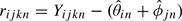to estimate the variance terms τ² and σ². Specifically, we define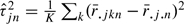d and 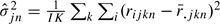, where and

With these estimates in place we were then ready to define a preprocessing procedure for single arrays and small batches. We motivate and describe these next.

2.1. fRMA algorithm

First, we background corrected each new array in the same manner as the training data set. Remember RMA background correction is a single-array method. Second, we quantile normalized each of the new arrays to the reference distribution created from the training data set. The final step was to summarize the probes in each probe set. Note that the arrays analyzed are not part of any of the batches represented in the training data set. For presentation purposes, we denote the new batch by l.

The first task in the summarization step was to remove the global batch effect from each intensity and create a probe-effect-corrected intensity:

The second task was to estimate the θs from these data using a robust procedure. A different approach was used for single-array summarization and batch summarization.

Single array.

Here, we dropped the i and l notation because we are analyzing only one array and one batch.

We estimated θ_n with a robust mean that weights each of the data points by the inverse of its variance:

The log gene expression was then estimated by the weighted mean:

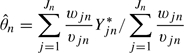with and w_jn, the weights obtained from an M-estimator procedure. This statistic has an intuitive interpretation—probes with large batch to batch (τ) or array to array (σ) variation should be down weighted, as well as, intensities that are outliers (small w).

Batch of arrays.

Here, we dropped the l notation because this method is intended to be applied to arrays from the same batch.

Note that the probe-effect-corrected data Y_jn^*≡{Y_ijn^*}_{i = 1,…,I} are correlated because they share the random effect γ_jn. We therefore implemented a robust procedure that accounts for this correlation. We rewrote Model (2.2) in matrix notation:

Here Y_n^*≡(Y_1,n^*,…,Y_Jn,n^*)^′ is a vector of all the probe-effect-corrected intensities for probe set n, θ≡(θ_1,n,…,θ_I,n)^′ are the parameters of interest, X≡1_{(Jn × 1)} ⊗ I_{(I × I)} is a matrix of indicator variables and δ is a vector of correlated errors with covariance matrix Σ≡(τ_1,n,…,τ_Jn,n)^′ × 1_{(1 × Jn)} ⊗ 1_{(I × I)} + (σ_1,n,…,σ_Jn,n)^′ × 1_{(1 × Jn)} ⊗ I_{(I × I)}. Here ⊗ is used to represent the Kronecker product. Note that the entries of Σ were estimated from the training set and treated as known. Therefore, we can easily rotate the intensities into independent identically distributed data: Z ≡ Σ ^{− 1/2}Y. We then estimated the transformed parameters Σ ^{− 1/2}θ using a standard M-estimator. Note that the final estimate can be expressed as a weighted least squares estimate:

with W a diagonal matrix of the weights obtained from the robust procedure.

This estimate also has an intuitive interpretation as probes with large correlation get down weighted and correlation is taken into account in the definition of distances used to define an outlier. Note that if just one of the entries of Y_jn^* is large in absolute value, it is likely an outlier, but, if all entries are large, it is probably due to a large batch-specific probe effect and is not considered an outlier.

3. RESULTS

To demonstrate the utility of the fRMA algorithm, we compared it to RMA. First, we assessed the preprocessing algorithms in terms of accuracy, precision, and overall performance as done by “affycomp” and “spkTools” (Irizarry and others, 2006), (McCall and Irizarry, 2008). Then, we assessed robustness to batch effects using 2 publicly available data sets.

We used the Affymetrix HGU133a spike-in data set to calculate measures of accuracy, precision, and overall performance. To assess accuracy, we calculated the “signal detection slope,” the slope from regressing observed expression on nominal concentration in the log₂ scale. It can be interpreted as the expected difference in observed expression when the true difference is a fold change of 2; as such, the optimal result is one. To assess precision, we computed the standard deviation of null log-ratios and the 99.5th percentile of the null distribution. Here “null” refers to the transcripts that were not spiked in and therefore should not be differentially expressed. The first precision measure is an estimate of the expected spread of observed log-ratios for nondifferentially expressed genes. The second precision measure assesses outliers; we expect 0.5% of nondifferentially expressed genes to exceed this value. Lastly, we calculated 2 measures of overall performance—the signal-to-noise ratio (SNR) and the probability of a gene with a true log₂ fold change of 2 being in a list of the 100 genes with the greatest fold change (POT). These measures were computed in 3 strata based on average expression across arrays. For a more detailed explanation of these measures, see McCall and Irizarry (2008).

First, the measures described above were calculated treating the data as a single batch; the results can be seen in Table 1. Then, the same data were preprocessed in the 3 original batches in which the data were generated; the results for these analyses can be seen in Table 2. In both tables, we also report the results from preprocessing the data with fRMA one array at a time. When the data were preprocessed as a single batch, RMA outperformed fRMA in the medium stratum based on SNR and POT. But in the low and high strata, RMA and fRMA performed comparably. When we processed the data in batches, fRMA outperformed RMA in all 3 strata primarily due to better precision.

Table 1.

For these results, we treated the spike-in data as a single batch. For each of the intensity strata, we report summary assessments for accuracy, precision, and overall performance. The first column shows the signal detection slope that can be interpreted as the expected observed difference when the true difference is a fold change of 2. In parenthesis is the standard deviation (SD) of the log-ratios associated with nonzero nominal log-ratios. The second column shows the SD of null log-ratios. The SD can be interpreted as the expected range of observed log-ratios for genes that are not differentially expressed. The third column shows the 99.5th percentile of the null distribution. It can be interpreted as the expected minimum value that the top 100 nondifferentially expressed genes will reach. The fourth column shows the ratio of the values in columns 1 and 2. It is a rough measure of SNR. The fifth column shows the probability that, when comparing 2 samples, a gene with a true log fold change of 2 will appear in a list of the 100 genes with the highest log-ratios. The preprocessing algorithm with the greatest SNR is displayed in bold

Low
Preprocessing	Accuracy	Precision		Performance
	slope (SD)	SD	99.5%	SNR	POT
RMA	0.25 (0.32)	0.10	0.36	2.50	0.36
fRMA—single array	0.25 (0.25)	0.11	0.45	2.27	0.22
fRMA—batch	0.26 (0.24)	0.10	0.36	2.60	0.33

Medium
Preprocessing	Accuracy	Precision		Performance
	slope (SD)	SD	99.5%	SNR	POT
RMA	0.83 (0.37)	0.09	0.40	9.22	0.88
fRMA—single array	0.82 (0.37)	0.10	0.49	8.20	0.82
fRMA—batch	0.80 (0.35)	0.09	0.44	8.89	0.85

High
Preprocessing	Accuracy	Precision		Performance
	slope (SD)	SD	99.5%	SNR	POT
RMA	0.57 (0.18)	0.06	0.22	9.50	0.97
fRMA—single array	0.58 (0.18)	0.06	0.23	9.67	0.98
fRMA—batch	0.62 (0.20)	0.07	0.25	8.86	0.97

Table 2.

Just as in Table 1 but processed in 3 batches then combined for analysis

Low
Preprocessing	Accuracy	Precision		Performance
	slope (SD)	SD	99.5%	SNR	POT
RMA	0.25 (0.32)	0.14	0.47	1.79	0.25
fRMA—single array	0.25 (0.25)	0.11	0.45	2.27	0.22
fRMA—batch	0.26 (0.26)	0.10	0.33	2.60	0.39

Medium
Preprocessing	Accuracy	Precision		Performance
	slope (SD)	SD	99.5%	SNR	POT
RMA	0.83 (0.39)	0.12	0.46	6.92	0.83
fRMA—single array	0.82 (0.37)	0.10	0.49	8.20	0.82
fRMA—batch	0.81 (0.36)	0.09	0.40	9.00	0.87

High
Preprocessing	Accuracy	Precision		Performance
	slope (SD)	SD	99.5%	SNR	POT
RMA	0.58 (0.20)	0.08	0.26	7.25	0.95
fRMA—single array	0.58 (0.18)	0.06	0.23	9.67	0.98
fRMA—batch	0.58 (0.20)	0.06	0.21	9.67	0.97

To assess the effect of combining data preprocessed separately, we created 2 artificial batches each containing the same 15 tissues from the E-AFMX-5 data set (Su and others, 2004) by randomly assigning one sample from each tissue type to each batch. We then analyzed each batch separately with RMA and fRMA. After obtaining a matrix of expression values for each batch, we performed hierarchical clustering on the combined expression matrix. Figure 4 shows that when the samples were preprocessed with RMA, they clustered based on the artificial batches, but when they were preprocessed with fRMA, they clustered based on tissue type.

Next, we compared batch effects using a publicly available breast cancer data set of 159 Affymetrix HGU133a arrays accessible at the NCBI GEO database (Edgar and others, 2002), accession GSE1456 (Pawitan and others, 2005). The dates on which the arrays were generated varied from June 18, 2002 to March 8, 2003. We grouped the data into 6 batches based on these dates (see Supplementary Table 2 available at Biostatistics online) and processed each batch separately using fRMA. We also processed the entire data set as one batch using RMA. Table 3 shows that there are statistically significant differences in average expression from batch to batch when the data are processed with RMA. These differences are not present when the data are analyzed using fRMA.

Table 3.

This table displays coefficients obtained from regressing gene expression on array batch. RMA shows a significant batch effect, while fRMA does not

RMA
Coefficients	Estimate	Standard Error	P-value
Intercept	6.758	0.003	< 0.001
Batch2	– 0.014	0.003	< 0.001
Batch3	0.002	0.004	0.658
Batch4	– 0.004	0.004	0.338
Batch5	– 0.010	0.003	0.004
Batch6	– 0.021	0.004	< 0.001

fRMA
Coefficients	Estimate	Standard Error	P-value
Intercept	7.183	0.002	< 0.001
Batch2	≈ 0.000	0.003	0.949
Batch3	≈ 0.000	0.003	0.937
Batch4	≈ 0.000	0.003	0.885
Batch5	≈ 0.000	0.003	0.968
Batch6	– 0.001	0.003	0.656

4. DISCUSSION

We have described a flexible preprocessing algorithm for Affymetrix expression arrays that performs well whether the arrays are preprocessed individually or in batches. The algorithm follows the same 3 steps as current algorithms: background correction, normalization, and summarization. Specifically, we have improved upon the summarization step by accounting for between-probe and between-batch variability.

Table 1 demonstrated that when analyzing batches of data together, RMA performed slightly better. Table 2 showed that when analyzing data in batches, fRMA consistently outperformed RMA. Specifically, fRMA showed greater precision than RMA.

Perhaps, the greatest disadvantage of multiarray preprocessing methods is the inability to make reliable comparisons between arrays preprocessed separately. Figure 4 showed the potentially erroneous results that one might obtain when combining data preprocessed separately. Furthermore, Table 3 showed that even if it were computationally feasible to preprocess all the data simultaneously with RMA, it would be unwise to do so due to batch effects. Unlike RMA, fRMA accounts for these batch effects and thereby allows one to combine data from different batches for downstream analysis.

As more data become publicly available, methods that allow simultaneous analysis of thousands of arrays become necessary to make use of this wealth of data. fRMA allows the user to preprocess arrays individually or in small batches and then combine the data to make inferences across a wide range of arrays. This ability will certainly prove useful as microarrays become more common in clinical settings.

The preprocessing methods examined here can be summarized based on what information they use to estimate probe effects. RMA uses only the information present in the data being currently analyzed; whereas fRMA utilizes both the information present in the data being analyzed and the information from the database. By using both sources of information, fRMA is able to perform well across a variety of situations.

The fRMA methodology can be easily extended to provide quality metrics for a single array. Brettschneider and others (2008) demonstrate that the normalized unscaled standard error (NUSE) can detect aberrant arrays when other quality metrics fail. The NUSE provides a measure of precision for each gene on an array relative to the other arrays. Precisions is estimated from the RMA model residuals. Therefore, the NUSE is multiarray on 2 counts. Using the fRMA methodology, one can develop a single-array version of NUSE. Precision can be estimated from the residuals described in Section 2 and the relative precision can be computed relative to all the arrays in the training data set.

Finally, note that fRMA requires a large database of arrays of the same platform. Currently, our software only handles 2 human arrays: HGU133a and HGU133Plus2. However, we have downloaded all available raw data (CEL) files for 5 other popular platforms and expect to have software for these in the near future.

FUNDING

National Institutes of Health (R01GM083084, R01RR021967 to R.A.I.); National Institute of General Medical Sciences (5T32GM074906 to M.M.).

References

- Affymetrix Inc. Guide to probe logarithmic intensity error (PLIER) estimation. Technical Note. 2005 [Google Scholar]
- Bolstad B. Berkeley, CA: University of California; 2004. Low-level analysis of high-density oligonucleotide array data: background, normalization and summarization, [PhD. Thesis] [Google Scholar]
- Bolstad B, Irizarry R, Astrand M, Speed T. A comparison of normalization methods for high density oligonucleotide array data based on variance and bias. Bioinformatics. 2003;19:185–193. doi: 10.1093/bioinformatics/19.2.185. [DOI] [PubMed] [Google Scholar]
- Brettschneider J, Collin F, Bolstad B, Speed T. Quality assessment for short oligonucleotide microarray data. Technometrics. 2008;50:241–264. [Google Scholar]
- Edgar R, Domrachev M, Lash A. Gene Expression Omnibus: NCBI gene expression and hybridization array data repository. Nucleic Acids Research. 2002;30:207. doi: 10.1093/nar/30.1.207. [DOI] [PMC free article] [PubMed] [Google Scholar]
- Fare T, Coffey E, Dai H, He Y, Kessler D, Kilian K, Koch J, LeProust E, Marton M, Meyer M and others. Effects of atmospheric ozone on microarray data quality. Analytical Chemistry. 2003;75:4672. doi: 10.1021/ac034241b. [DOI] [PubMed] [Google Scholar]
- Gautier L, Cope L, Bolstad B, Irizarry R. affy–analysis of Affymetrix GeneChip data at the probe level. Bioinformatics. 2004;20:307–315. doi: 10.1093/bioinformatics/btg405. [DOI] [PubMed] [Google Scholar]
- Huber P, Wiley J, InterScience W. Robust Statistics. New York: Wiley; 1981. [Google Scholar]
- Irizarry R, Hobbs B, Collin F, Beazer-Barclay Y, Antonellis K, Scherf U, Speed T. Exploration, normalization, and summaries of high density oligonucleotide array probe level data. Biostatistics. 2003;4:249. doi: 10.1093/biostatistics/4.2.249. [DOI] [PubMed] [Google Scholar]
- Irizarry R, Warren D, Spencer F, Kim I, Biswal S, Frank B, Gabrielson E, Garcia J, Geoghegan J, Germino G, et al. Multiple-laboratory comparison of microarray platforms. Nature Methods. 2005;2:345–350. doi: 10.1038/nmeth756. [DOI] [PubMed] [Google Scholar]
- Irizarry R, Wu Z, Jaffee H. Comparison of Affymetrix GeneChip expression measures. Bioinformatics. 2006;22:789–794. doi: 10.1093/bioinformatics/btk046. [DOI] [PubMed] [Google Scholar]
- Katz S, Irizarry R, Lin X, Tripputi M, Porter M. A summarization approach for Affymetrix GeneChip data using a reference training set from a large, biologically diverse database. BMC Bioinformatics. 2006;7:464. doi: 10.1186/1471-2105-7-464. [DOI] [PMC free article] [PubMed] [Google Scholar]
- Li C, Wong W. Model-based analysis of oligonucleotide arrays: expression index computation and outlier detection. Proceedings of the National Academy of Sciences. 2001;98:31. doi: 10.1073/pnas.011404098. [DOI] [PMC free article] [PubMed] [Google Scholar]
- McCall M, Irizarry R. Consolidated strategy for the analysis of microarray spike-in data. Nucleic Acids Research. 2008;36:e108. doi: 10.1093/nar/gkn430. [DOI] [PMC free article] [PubMed] [Google Scholar]
- Parkinson H, Kapushesky M, Kolesnikov N, Rustici G, Shojatalab M, Abeygunawardena N, Berube H, Dylag M, Emam I, Farne A and others. ArrayExpress update–from an archive of functional genomics experiments to the atlas of gene expression. Nucleic Acids Research. 2008;37:D868–D872. doi: 10.1093/nar/gkn889. [DOI] [PMC free article] [PubMed] [Google Scholar]
- Pawitan Y, Bjöhle J, Amler L, Borg A, Egyhazi S, Hall P, Han X, Holmberg L, Huang F, Klaar S and others. Gene expression profiling spares early breast cancer patients from adjuvant therapy: derived and validated in two population-based cohorts. Breast Cancer Research. 2005;7:R953–R964. doi: 10.1186/bcr1325. [DOI] [PMC free article] [PubMed] [Google Scholar]
- Su A, Wiltshire T, Batalov S, Lapp H, Ching K, Block D, Zhang J, Soden R, Hayakawa M, Kreiman G and others. A gene atlas of the mouse and human protein-encoding transcriptomes. Proceedings of the National Academy of Sciences. 2004;101:6062–6067. doi: 10.1073/pnas.0400782101. [DOI] [PMC free article] [PubMed] [Google Scholar]
- Tukey J. Exploratory Data Analysis. Reading, MA: Addison-Wesley; 1977. [Google Scholar]
- Wu Z, Irizarry R, Gentleman R, Martinez-Murillo F, Spencer F. A model-based background adjustment for oligonucleotide expression arrays. Journal of the American Statistical Association. 2004;99:909–917. [Google Scholar]
Associated Data
This section collects any data citations, data availability statements, or supplementary materials included in this article.