Measuring morphological features using light-scattering spectroscopy and Fourier-domain low-coherence interferometry

Abstract

We present measurements of morphological features in a thick turbid sample using light-scattering spectroscopy (LSS) and Fourier-domain low-coherence interferometry (fLCI) by processing with the dual-window (DW) method. A parallel frequency domain optical coherence tomography (OCT) system with a white-light source is used to image a two-layer phantom containing polystyrene beads of diameters 4.00 and 6.98 μm on the top and bottom layers, respectively. The DW method decomposes each OCT A-scan into a time–frequency distribution with simultaneously high spectral and spatial resolution. The spectral information from localized regions in the sample is used to determine scatterer structure. The results show that the two scatterer populations can be differentiated using LSS and fLCI.

Light-scattering spectroscopy (LSS) [1] has served as the foundation for a number of technologies, including Fourier-domain low-coherence interferometry (fLCI) [2], which has been developed to measure the enlargement of epithelial cell nuclei associated with precancerous development [3]. In fLCI, depth resolution is obtained by coherence gating with spectral information acquired using a short-time Fourier transform (STFT). This process is similar to what is done in spectroscopic optical coherence tomography (SOCT) [4]. However, in fLCI, after processing with a STFT, the spectrum from a given depth is analyzed to determine the size of scattering objects [2].

SOCT, an extension of optical coherence tomography (OCT), provides the same cross-sectional tomographic imaging capabilities [5] with the added benefit of spectroscopic-based contrast[4]. As described above, SOCT uses STFTs or wavelet transforms to obtain spectroscopic information, which provides additional information about a sample. Unfortunately, the windowing process of STFTs introduces an inherent trade-off between spatial and spectral resolution, which limits further quantitative processing of the depth-resolved spectra. Recently, we introduced the dual window (DW) method for processing SOCT signals, which achieves both high spectral and high spatial resolution, allowing for a thorough quantitative treatment of the depth-resolved spectral information [6].

In this Letter, we present morphological measurements of different populations of scatterers in a turbid medium by processing with the DW method and analyzing with LSS and fLCI techniques. The DW method decomposes each depth-resolved A-scan from the OCT signal into a time–frequency distribution (TFD), which inherently aligns the quantitative spectral analysis with the OCT image to determine the local scatterer structure. The approach is demonstrated through imaging and analysis of a two-layer phantom, with each layer containing a suspension of different size polystyrene beads.

A white light parallel frequency domain OCT system, as described by Graf et al. [7], is used. In short, a Michelson interferometer geometry is modified with four additional lenses to form a 4f imaging system, thereby limiting the number of spatial modes illuminating the sample and reference arm. The light returned by the two arms are combined and imaged onto the entrance slit of an imaging spectrograph. The interference signal is obtained in parallel across 150 spatial channels along the entrance slit of the spectrograph, spanning 3.75 mm, each channel with a lateral resolution of 26 μm. The spectrograph disperses each channel into its wavelength components with a spectral resolution of 0.1 nm. For this configuration, the 136.9 nm bandwidth centered at λ₀ =565.4 nm yields a theoretical axial resolution of 1.03 μm, which agrees reasonably well with the experimentally measured resolution of 1.22 μm.

To process the OCT image, six steps are taken. (1) The sample and reference arm intensities are acquired separately and subtracted from the signal. (2) The resulting interferometric signal is divided by the intensity of the reference field to normalize for the source spectrum and detector efficiencies as a function of λ. This step is of particular importance for quantitative comparison of depth-resolved spectra, since the remaining spectral dependence is assumed to arise solely from absorption of forward scattered light and scattering cross sections of backscattered light. (3) The data are resampled into a linear wave-number vector, k=2π/λ. (4) Chromatic dispersion is digitally corrected as described by Zhu et al. [8]. (5) A fast Fourier transform is executed to obtain an A-scan, and (6) the process is repeated for each of the 150 spatial channels to obtain the image.

Similar to the generation of the OCT image, the DW uses the interferometric information and requires steps (1)–(4) as described above. As a last step, a product of two STFTs is taken: one with a narrow window for high spectral resolution and another with a wide window for high spatial resolution. Equation (1) (adapted from [6]) describes the distribution obtained with the DW from a single spatial channel:

$$\begin{array}{l}=\int 2\langle E_S\rangle cos({\kappa }_1·\mathrm{\Delta }\text{OPL})e^{-{({\kappa }_1-k)}^2/2a^2}{e}^{-i{\kappa }_{1}z}\text{d}{\kappa }_1\\ \times \int (2\langle E_s\rangle cos({\kappa }_2·\mathrm{\Delta }\text{OPL})e^{-{({\kappa }_2-k)}^2/2b^2}{e}^{-i{\kappa }_{2}z})\ast \text{d}{\kappa }_2\end{array}$$ (1)

where E_S denotes the sample field, 〈···〉 denotes an ensemble average, ΔOPL is the optical path length difference between the sample and reference arms, z is the axial distance, and a and b are the standard deviations of the windows. Robles et al. have shown that the DW, a product of two linear operations, can be described by Cohen’s class bilinear functions [6]. With b ≫ a, the DW samples the Wigner TFD with two orthogonal windows that are independently set by the parameters a and b, resulting in a suppression of many common artifacts.

The DW contains two components that relay information, which are analyzed independently. The first component, contained in the low frequencies of DW(k,z₀), corresponds to the spectral dependence of the optical signal at z₀ and arises from absorption and scattering in the sample. This component is analyzed with LSS. The second component is the morphological features about z₀, arising from the temporal coherence of the scattered light and contained in the local oscillations (high frequencies) of the signal [6]. This component is analyzed with fLCI.

This study seeks to analyze scattering structures in a thick turbid sample using LSS and fLCI methods. Thus, a two-layer phantom containing polystyrene beads (n_b =1.59) of different sizes suspended in a mixture of agar (2% by weight) and water, with n_a =1.35, is used. The bead diameter in the top layer is d=4.00±0.033 μm, and in the bottom layer d =6.98±0.055 μm, with both bead distributions possessing a standard deviation of 1% in size. The scatterer concentration is chosen to yield a mean-free scattering path length of l_s =1 mm to ensure a sufficient signal-to-noise ratio (SNR) at deeper depths. Figure 1(a) shows an OCT image of the phantom acquired by a single 0.3 s exposure, with no scanning needed.

Fig. 1.

(a) Parallel frequency-domain OCT image of a two-layer phantom. The top layer (optical path length difference/2 (ΔOPL/2) ranging from 35 to 125 μm) contains 4.00 μm beads, while the bottom layer (400–550 μm) contains 6.98 μm beads. The dashed red line corresponds to a single lateral channel from which the TFD illustrated in Fig 2 is generated. (b) Overlay of the fLCI measurements with the OCT image. Scatterers without color coding correspond to points that produced nonunique size measurements.

The DW method is used to calculate a TFD for each lateral channel, yielding a spectrum for each pixel in the image with high spectral and spatial resolution (parameters set to a=0.0454 μm⁻¹ and b =0.6670 μm⁻¹). Figure 2(a) shows a processed TFD of a representative channel [red dashed line in Fig. 1(a)], with the corresponding A-scan [Fig. 2(b)]. Two representative points are selected, and the spectrum from each is analyzed as an example. Figures 3(a) and 3(b) give the spectral profiles (solid curves) from points 1 and 2, respectively.

Fig. 2.

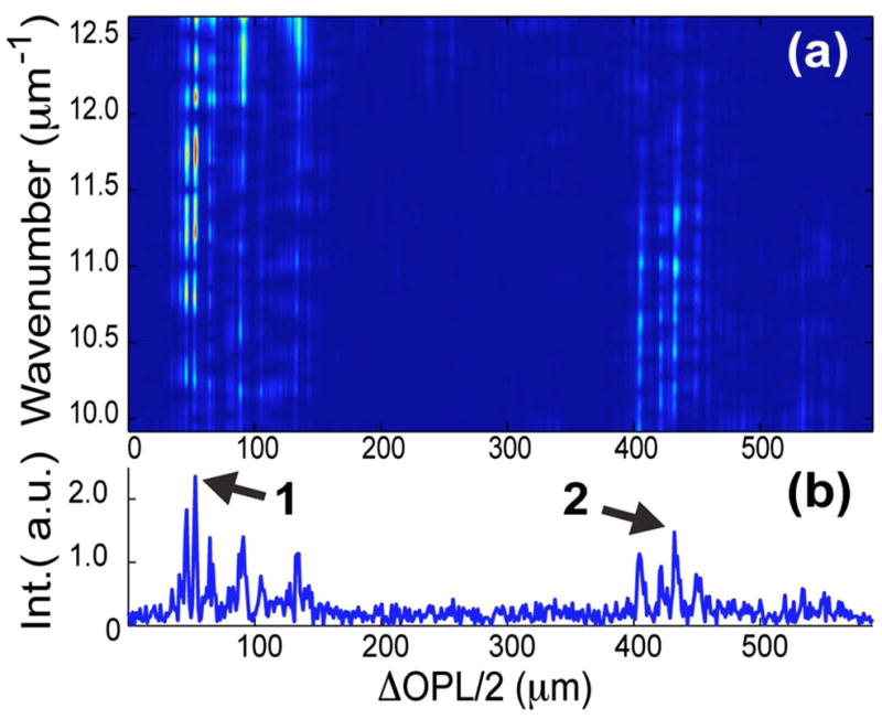
(Color online) (a) TFD using the DW method generated from a single representative lateral channel from the OCT image [dashed red line in Fig 1(a)]. (b) Corresponding A scan. Points 1 and 2 identify representative points of interest to be analyzed with LSS and fLCI.

Fig. 3.

(Color online) (a)–(b) DW spectral profiles (blue curves) and low-pass filtered spectra (dotted green curves) from points 1 and 2 in Fig. 2(b), respectively. Dashed red curves are the theoretical scattering cross sections for 3.97 and 6.91 μm spherical scatterers for points 1 and 2, respectively, obtained by least-squares fitting the low-pass filtered spectrum. (c)–(d) Correlation function from points 1 and 2, with correlation distances (d_c) of 4.25 and 6.87 μm, respectively.

The low frequencies of the depth-resolved spectra contain information about absorption and scattering cross sections. Since no chromophores are present, the spectral dependence gives the scattering cross section of the beads; thus, the Van de Hulst approximation [9] can be used to determine the bead size. To achieve this, the DW spectral profile is low-pass filtered with a hard cutoff frequency of 3.5 μm (three cycles); then, a least-squares fit is used to obtain the scatterer diameter. In Figs. 3(a) and 3(b), the dotted green curves show the low-pass filtered data used for fitting, which yield d₁ =3.97 μm and d₂ =6.91 μm for points 1 and 2, respectively, in good agreement with the true bead sizes. The dashed red curves give the theoretical scattering cross section corresponding to the best fits: note that these are in excellent agreement with the processed signals.

The high-frequency components of DW(k,z₀) give the fLCI measurement. First, the spectral dependence is removed by subtracting the line of best fit from the LSS analysis above. Then, the residuals are Fourier transformed to yield a correlation function. The maxima of this function give the differences in optical path length between dominant scattering features in the analyzed region. For the bead phantom, the local oscillations predominately result from scattering by the front and back surfaces of a single bead, and thus the correlation function maximum indicates the round-trip optical path length through the scatterer. Simulated OCT images by Yi et al. [10] show that light scattered by a single microsphere gives rise to multiple peaks at longer correlations, which are also seen in our data. Figures 3(c) and 3(d) plot the correlation function for points 1 and 2 respectively, giving correlation peaks at d_c = ΔOPL/(2n_b) =4.25 μm and 6.87 μm, in good agreement with both the LSS measurements and true bead sizes.

The procedure was repeated for all points in the OCT image, where an automated algorithm selected peaks that were above a threshold (intensity >10) and 10% higher than any other maxima in the correlation function. Further, only points where the LSS and fLCI measurements were in agreement within the system’s resolution (±1.22 μm) were included in the analysis, with the remaining points omitted. Prior to the last criteria, the LSS and fLCI measurements showed 82% agreement in the top layer and a lower 35% agreement in the bottom layer owing to the lower SNR at deeper sample depths. Figure 1(b) shows an overlay of the fLCI measurements that pass all the algorithm criteria with the OCT image. The LSS map (not shown) yields similar results, since the LSS and fLCI measurements were required to be in agreement for inclusion. In the top layer, the average scatterer size was 3.82±0.67 μm and 3.68 ±0.41 μm for the fLCI and LSS measurements, respectively (112 points). In the bottom layer, the average scatterer size was 6.55±0.47 μm and 6.75± 0.42 μm for fLCI and LSS, respectively (113 points). These results show that by utilizing two independent methods to analyze scattering structure (fLCI and LSS), our technique yields accurate and precise measurements throughout the whole OCT image. Sources of error for the fLCI measurement can arise owing to partial volume effects where multiple beads lie within a single pixel region (26 μm×1.15 μm), giving multiple maxima in the correlation function.

In summary, by processing with the DW method, the LSS and fLCI measurements yield results consistent with the morphological features of the multilayer scattering sample. Recently, Yi et al. presented results that use a similar optical system and STFT processing to discriminate fluorescent and non-fluorescent microspheres in a weakly scattering medium [10]. Their analysis was restricted to a thin (<100 μm) layer and did not assess structure, as they intentionally discarded the high-frequency spectral modulations due to the scatterer’s structure (i.e., diameter). In comparison, the results presented here confirm the potential to measure enlargement of epithelial cell nuclei, which are nonabsorbing, to detect precancerous development [11] within intact tissues.

References

- 1.Perelman LT, Backman V, Wallace M, Zonios G, Manoharan R, Nusrat A, Shields S, Seiler M, Lima C, Hamano T, Itzkan I, Van Dam J, Crawford JM, Feld MS. Phys Rev Lett. 1998;80:627. [Google Scholar]
- 2.Graf RN, Wax A. Opt Express. 2005;13:4693. doi: 10.1364/opex.13.004693. [DOI] [PMC free article] [PubMed] [Google Scholar]
- 3.Kumar V, Abbas AK, Fausto N. Robbin and Cotran Pathologic Basis of Disease. Elsevier/Saunders; 2005. [Google Scholar]
- 4.Morganer U, Drexler W, Kärtner FX, Li XD, Pitris C, Ippen EP, Fujimoto JG. Opt Lett. 2000;25:111. doi: 10.1364/ol.25.000111. [DOI] [PubMed] [Google Scholar]
- 5.Huang D, Swanson EA, Lin CP, Schuman JS, Stinson WG, Chang W, Hee MR, Flotte T, Gregory K, Puliafito CA, Fujimoto JG. Science. 1991;254:1178. doi: 10.1126/science.1957169. [DOI] [PMC free article] [PubMed] [Google Scholar]
- 6.Robles F, Graf RN, Wax A. Opt Express. 2009;17:6799. doi: 10.1364/oe.17.006799. [DOI] [PMC free article] [PubMed] [Google Scholar]
- 7.Graf RN, Brown WJ, Wax A. Opt Lett. 2008;33:1285. doi: 10.1364/ol.33.001285. [DOI] [PMC free article] [PubMed] [Google Scholar]
- 8.Zhu Y, Terry N, Wax A. Opt Lett. 2009;34:3196. doi: 10.1364/OL.34.003196. [DOI] [PMC free article] [PubMed] [Google Scholar]
- 9.Van de Hulst HC. Light Scattering by Small Particles. Dover; 1957. pp. 173–199. [Google Scholar]
- 10.Yi J, Gong J, Li X. Opt Express. 2009;17:13157. doi: 10.1364/oe.17.013157. [DOI] [PubMed] [Google Scholar]
- 11.Graf RN, Robles FE, Wax A. J Biomed Opt. 2009;14:064030. doi: 10.1117/1.3269680. [DOI] [PMC free article] [PubMed] [Google Scholar]