Functional and effective connectivity of visuomotor control systems demonstrated using generalized partial least squares and structural equation modeling

Abstract

Tasks employing parametric variation in movement rate are associated with predictable modulations in neural activity and provide a convenient context for developing new techniques for system identification. Using a multistage approach, we explored the functional and effective connectivity of a visuomotor control system by combining generalized partial least squares (gPLS) with subsequent structural equation modeling (SEM) to reveal the relationships between neural activity and finger movement rate in an experiment involving visually paced left or right thumb flexion. The gPLS in the first analysis stage automatically identified spatially distributed sets of BOLD‐contrast signal changes using linear combinations of sigmoidal basis functions parameterized by kinematic variables. The gPLS provided superior sensitivity in detecting task‐related functional activity patterns via a step‐wise comparison with both classical linear modeling and behavior correlation analysis. These activity patterns were used in the second analysis stage, which employed SEM to characterize the areal regional interactions. The hybrid gPLS/SEM procedure allowed modeling of complex regional interactions in a network including primary motor cortex, premotor areas, cerebellum, thalamus, and basal ganglia, with differential activity modulations with respect to rate observed in the corticocerebellar and corticostriate subsystems. This effective connectivity analysis of visuomotor control circuits showed that both the left and right corticocerebellar and corticostriate circuits exhibited movement rate‐related modulation. The identification of the functional connectivity among regions participating particular classes of behavior using gPLS, followed by the estimation of the effective connectivity using SEM is an efficient means to characterize the neural interactions underlying variations in sensorimotor behavior. Hum Brain Mapp, 2009. © 2009 Wiley‐Liss, Inc.

INTRODUCTION

The neural systems responsible for integrating perception and action exhibit a high degree of interaction and mutual influence, when operating under changing task requirements. In describing the spatial and temporal interactions and complex modulatory influences underlying these phenomena, a distinction is commonly drawn between two types of regional interaction, functional and effective connectivity. Although functional connectivity refers to the temporal correlation between regional brain activity and an effect of interest, including relevant stimulus or task characteristics [Friston et al., 1993], effective connectivity refers to the directional influences among brain regions [Friston et al., 1997]. To achieve an integrated network analysis of both functional and effective connectivity in neural systems controlling complex behavior, it is critical to first accurately identify the spatially distributed regions that are functionally active with respect to the relevant task properties. Only after successful identification of the “nodes” comprising a functional neural network it is possible to undertake accurate modeling of their effective connectivity. As details of the spatial distribution of task‐related activity are likely to carry important information about the organization of the neural subsystems underlying complex behavior, the application of multivariate methods could have significant advantages in identifying the locations of the regionally specialized areas used in modeling the quantitative relationship between regional neural activity measured with functional magnetic resonance imaging (fMRI) and quantitative measures of task performance.

Tasks that can be parametrically varied with respect to stimulus properties or performance rate provide a convenient means to study modulation of regional interactions. For example, control of voluntary movement requires a high degree of process integration across a spatially distributed network of functionally specialized cortical and subcortical brain structures [Kandel et al., 2000; Nolte, 1998]. Previous positron emission tomography (PET) [Colebatch et al., 1991; Fox et al., 1985], and fMRI [Le Bihan and Karni, 1995; Rao et al., 1993] studies have demonstrated that the processes responsible for sensorimotor coordination span many brain structures, including primary sensorimotor cortex, lateral and medial premotor areas, and subcortical areas including the thalamus, putamen and cerebellum [Grafton et al., 1992; VanMeter et al., 1995]. Other neuroimaging studies of the motor system have employed repetitive finger movement tasks to study the spatial distribution of task‐related activity [Le Bihan and Karni, 1995; Rao et al., 1995], the differential responses related to movement complexity [Grafton et al., 1992; Rao et al., 1993; Wexler et al., 1997], and the correspondence between movement rate and neural activity [Rao et al., 1996; Sadato et al., 1996b; Schlaug et al., 1996; VanMeter et al., 1995]. Of particular interest in the present context is that early PET studies showed that regional cerebral blood flow (rCBF) in primary sensorimotor cortex was linearly dependent on manual movement rate [Sadato et al., 1996b; VanMeter et al., 1995], and subsequent fMRI studies have demonstrated the existence of both linear and nonlinear relationships between blood oxygen level dependent (BOLD) contrast in primary motor cortex and movement rate [Rao et al., 1996; Sadato et al., 1997; Schlaug et al., 1996]. In contrast, other cortical motor areas, including lateral and medial premotor cortex, have repeatedly been shown to have nonlinear rate‐dependent responses using either PET [Sadato et al., 1996b; VanMeter et al., 1995] or BOLD‐contrast fMRI [Agnew et al., 2004; Riecker et al., 2003; Schlaug et al., 1996]. Thus, when studied with a variety of functional neuroimaging techniques, parametric modulation of movement rate has been associated with reliable linear and nonlinear modulations in neural activity, making this class of tasks an excellent choice to explore novel methods for the identification and characterization of regional interactions.

In our previous work using a traditional univariate modeling approach, we examined the quantitative relationship between regional brain activity and movement rate, finding that the structures comprising the lateralized corticocerebellar and corticostriatal networks were differentially modulated during performance of variable rate repetitive finger movements of the left or right hand [Agnew et al., 2004]. In this article, we continue this analysis by demonstrating the utility of combining generalized partial least squares (gPLS) analysis and structural equation modeling (SEM) to more fully characterize the interactions among the neural subsystems controlling visuomotor task performance using, as an example, activity recorded during visually paced, variable‐rate, finger movements.

In this context, functional connectivity analysis using gPLS has particular advantages. gPLS is a robust multivariate modeling algorithm derived from the partial least squares (PLS) approach [Lin et al., 2003; McIntosh et al., 1996a], taking advantage of its inherent computational efficiency and flexibility in accommodating simultaneous multiple‐contrast comparisons. Our gPLS analysis framework utilizes psychometric sigmoidal basis functions that can efficiently span the target behavioral measurement space. This novel modeling approach enables direct detection of relationships between neuroimaging data time series and behavioral measurements made across varying spatiotemporal scales and is therefore especially suitable for neuroimaging experiments with parametric designs. In addition, gPLS analysis of functional connectivity has particular advantages over voxel‐wise mass univariate approaches, which ignore the functional connectivity among brain regions in the characterization of neural response patterns [Friston et al., 1995].

After identifying the spatially distributed collection of areas exhibiting task‐related activity using gPLS, we next use SEM to characterize the modulation of directional influences among the activated regions during conditions of varying movement rate. This combination of multivariate functional connectivity analysis with subsequent effective connectivity analysis represents an integrated approach to the characterization of large‐scale neural network interactions. The resulting model includes both “nodes” (active areas) and directional “paths” (connections modulating the active areas), which together constitute the “neural context” of the functioning sensorimotor system.

METHODS

Overview

The overall analysis procedure comprised a two‐step network modeling approach that begins with functional connectivity analysis using gPLS, to identify the spatial distribution of functionally specialized regions, followed by effective connectivity analysis using SEM to quantify directional influences among the active regions. We first demonstrate the advantages of the multivariate gPLS approach using a set of sigmoidal basis functions to model the movement behavior with kinematic data from a variable‐rate repetitive finger flexion experiment. We then compare the results obtained with this sigmoidal basis set with simpler models using a step‐wise univariate analysis incorporating regressors that include constant functions, linear functions, sigmoidal functions, and a reference vector derived from the observed pattern of task‐related signal change in contralateral primary motor cortex. The results of the univariate modeling comparison show that the highest detection sensitivity is obtained when using the sigmoidal basis set. We next use the functional connectivity estimates resulting from the gPLS procedure to construct a structural equation model designed to reveal changes in interregional directional interactions in the corticocerebellar and corticostriatal visuomotor control subsystems during variable rate movements made with the left or right hands.

Experimental Design and Image Acquisition

Twelve right handed participants (five male, seven female; average age, 27.6 years; range, 18–39) participated in this study. All gave written informed consent and were compensated for their participation under terms approved by the local Institutional Review Board. Individuals with neurological or medical conditions known to affect brain function or first‐degree relatives with neurological, psychiatric, or developmental disorders were excluded from the study. Current use of psychoactive or vasoactive medications was grounds for exclusion, as was the presence of implanted electronic devices or ferromagnetic material. After the initial screening, hand preference was measured using the Edinburgh Handedness Scale (EHS) [Oldfield, 1971]. Scores on this instrument can range from −100 for a completely left handed participant to +100 for a completely right handed participant. All participants in this study were strongly right handed with an average EHS score of 93 and a standard deviation of 14.

Our nested block design involved two factors, hand (left or right), and movement rate (0.3Hz, 1.0 Hz, or 3.0 Hz). The task required executing paced thumb flexions in response to a repeating visual stimulus. Before entering the MRI system, participants were trained on the task until stable performance was achieved using the same response device later used inside the MRI system. Stimuli consisted of a fixation cross and, during the task condition, a bright 2° annulus that flashed around the fixation mark for 100 ms. Participants were instructed to execute a button press in time with the flashing annulus, while their response time and accuracy were recorded. To achieve a broad performance range that included relatively rapid repetitive movements, we employed a pacing task, rather than a stimulus‐response task. The right or left thumb was used to respond in alternate runs.

Data were collected in 6 runs during a single imaging session. During the course of the experiment, participants lay supine in the MRI system and viewed pacing stimuli that were projected onto a rear‐projection screen, executing movements with either the dominant (right) or nondominant (left) thumb at three different rates: 0.3 Hz, 1.0 Hz, and 3.0 Hz, which were randomized across runs. For the movement conditions, participants were instructed to respond in time with the stimulus, using the thumb specified by the experimenter at the beginning of that run. During the fixation condition, participants were instructed to lie still, relax, and focus on the fixation cross. Each acquisition run consisted of 10 cycles of alternating movement and fixation, with 12 images per cycle. Kinematic data were recorded to assess task compliance, and multislice echo‐planar image (EPI) acquisition was employed (TE = 43 ms, TR = 4.2 s, 64 × 64 matrix, 230 mm FOV, 46 axial slices, 3.6 mm cubic voxels, 128 time points per run, with eight dummy scans preceding data collection) using a 1.5 Tesla MRI system (Vision, SIEMENS Medical Solutions, Erlangen, Germany). Analysis of these data using traditional mass univariate regression techniques has been previously reported [Agnew et al., 2004].

Data Preprocessing

The EPI time series were processed using MEDx 3.28 (Sensor Systems, Sterling, VA). To correct for interscan head motion effects, each EPI volume was registered to the mean of its time series using a linear 6 parameter rigid‐body transformation model employing a least‐squares fitting technique. Image volumes were then resampled using chirp‐z interpolation. Global intensity variations were corrected with image intensity rescaling, performed by computing the ratio that relates mean image intensity in a particular volume to an arbitrary value of 1,000. Low‐frequency temporal signal fluctuations were removed by application of a high‐pass filter with the frequency cutoff set at twice the task cycle time period (two blocks × 4.2 s per TR × 12 TRs per block = 100.8 s). Next, a 3D Gaussian filter (FWHM = 6 mm in all dimensions) was applied to each volume in the time series. To facilitate estimation of group effects, the mean EPI image from each run was registered to the MNI EPI template provided with SPM99 using AIR 3.08 with 12 degrees of freedom. The resulting transformation matrix was saved and applied to the task vs. control contrast images derived from each run.

We created two separate matrices for the image data collected during movements executed with either hand, pooled across movement rates and participants. For each participant, we derived a contrast image, for each movement rate and hand, by determining the difference between the mean task (movement) and control (fixation) conditions. To account for delays in neurovascular coupling, each hemodynamic time series was shifted by one TR (4.2 s) relative to the task onset. The resulting whole‐brain contrast images were then reorganized into one row vector in the data matrix. The overall model consisted of three conditions (0.3 Hz, 1.0 Hz, and 3.0 Hz movement rates) with 12 participants, totaling 36 rows in each of the two data matrices representing task‐related modulation related to left and right hand movement.

Functional Connectivity Estimated by Generalized Partial Least Squares Analysis

Here, we present the gPLS formulation used to detect loci of activity used to construct the model employed in the subsequent effective connectivity analysis. Beginning with a brief review of PLS methods, we describe how the gPLS framework employs basis functions to characterize spatiotemporal patterns of activity in neuroimaging data. Our approach to basis function selection is described with a particular emphasis on the use of sigmoidal basis functions to efficiently model parametrically varying behavior. Basis function optimization was done using cross validation. Given a particular set of basis functions, we then made statistical inferences using nonparametric permutation and bootstrap procedures. A schematic diagram of the gPLS analysis procedure is shown in Figure 1.

Figure 1.

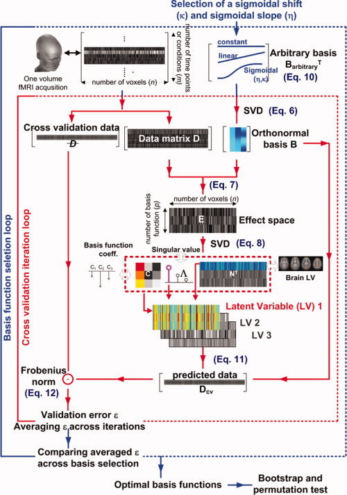
Schematic diagram of the gPLS analysis, including choice of basis functions, cross validation procedure, and PLS decomposition of the effect space created from the crosscovariance between the neuroimaging data and a model. The dark blue text in parentheses indicates the corresponding formula used in the Methods and Appendix sections. The gPLS analysis procedure includes choice of basis functions, identification of spatiotemporal model parameters, and cross validation components. [Color figure can be viewed in the online issue, which is available at www.interscience.wiley.com.]

PLS background

To introduce the gPLS procedure, we present a description of PLS methods as they have been applied in functional neuroimaging studies [McIntosh et al., 1996a]. A more detailed review is also available [McIntosh and Lobaugh, 2004]. PLS is commonly used to identify a linear model describing a set of predicted variables in terms of other observable variables, employing latent variables to model the covariance structure in the two variable spaces. In other words, PLS can find the best orthogonal linear combination of a particular basis set for predicting task‐related modulations in activity. In the PLS framework, functional neuroimaging experiments can be modeled with both a spatiotemporal neuroimaging data matrix D of m time points and n image voxels and a contrast matrix Π of m time points and d conditions. The effect space E can be constructed by crosscorrelating D and Π:

(1)

E is a partial crosscorrelation matrix consisting of projections of the temporal information in the data matrix D into different conditions encoded in columns of the design matrix Π, the so‐called “projection into latent structures” operation that provides an alternate source for the PLS acronym. Note that the projection operation helps to reduce the dimensionality of E dramatically compared with D. Next, we employ singular value decomposition (SVD) to decompose the effect space:

(2)

where U and V ^T are singular vector matrices of dimensions d × p and p × n, respectively. Λ is a p × p diagonal singular value matrix describing the significance of each spatiotemporal model, which consists of one column of U and one row of V ^T. Using a least squares approximation, the SVD decomposes spatiotemporal models inside the effect space E, a partial correlation matrix from which the name PLS is derived.

Generalized partial least squares analysis

gPLS analysis partitions the neuroimaging data into the linear combination of parameterized spatiotemporal models. This approach is different from the standard PLS analysis, where neuroimaging data are directly decomposed into spatiotemporal models without incorporating any behavioral information into the model. Specifically, we assume that the spatiotemporal functional imaging data D consists of a set of uncorrelated spatiotemporal models:

(3)

where M and N ^T are unitary matrices of dimensions m × p and p × n, respectively. They respectively represent p uncorrelated models in time and space, with p ≤ m,n. Again, Λ is a p × p diagonal matrix describing the significance of each spatiotemporal model, which consists of one column of M and one row of N ^T. X represents the residuals. We further decompose the temporal models M into linear combinations of the basis function matrix B:

(4)

Columns of B are basis functions for the individual column of M. C is the matrix of unknown basis coefficients. Without loss of generality, we assume that the basis functions are orthonormal. Orthonormal basis functions can be derived from generic nonorthonormal bases using SVD.

(5A)

An arbitrary choice of basis functions (columns of B _arbitrary) can thus be transformed into orthonormal ones as:

(5B)

The temporal model M can be written explicitly using an arbitrary basis family

(6)

In this article, we used sigmoidal functions parameterized by the finger movement rates to construct B _arbitrary. Further details of the basis function selection are described in the “gPLS basis set selection” section below.

Identification of the basis coefficients C was done by following the standard PLS analysis procedure. An effect space E was first constructed by projecting the data matrix onto these bases.

(7)

SVD was used to decompose the effect space E to reveal the basis function coefficients C and their spatial loading N.

(8)

Each column of the coefficient matrix C, along with the whitened basis matrix B, constitutes the temporal characterization of a spatiotemporal model M. Each row of the matrix N ^T quantifies the spatial loading of the same model. Using the terminology of standard PLS analysis, each column of C is called a temporal latent variable (temporal LV), and each row of N ^T is called a spatial latent variable (spatial LV). We can also derive the “spatial scores” and “temporal scores” as:

(9)

It follows that each column of the temporal score represents a temporal characterization of one spatiotemporal model. Examining both temporal scores and spatial LVs using prior knowledge about the experiment design and the neuroanatomical distribution of effects provides the foundation for explanatory inferences about, and confidence in, the identified spatiotemporal models. In this multivariate modeling approach, temporal scores and spatial LVs predict the functional image signals under various conditions occurring at different times. If the basis functions are continuous, we can further exploit that property to reveal the relationship between neural activity and experimental conditions or time by interpolating and extrapolating the temporal LVs, a process discussed in the “gPLS model cross validation” section later. Singular values are normalization factors used to scale temporal and spatial LVs to the original data matrix.

gPLS basis set specification

For the spatiotemporal gPLS modeling procedure, we included constant, linearly rate dependent, and sigmoidal functions with different transition slopes () and shifts (), in order to build a basis set b modeling the fMRI time series, based on the movement rate . These three basis functions constitute the matrix B _arbitrary in [Eq. (5A)]. The sigmoidal functions are written explicitly as:

(10)

As b is unitless and r is in units of Hz, κ has units of Hz, and η has units of Hz⁻¹. The transition slopes of sigmoid functions used were 1, 2, 4, and 8; the shifts of the sigmoidal functions were 0.0, 0.3 1.0, 2.0, and 3.0. These transition slopes and shifts give rise to the corresponding basis functions shown in Figure 2A. We were inspired by the results of our previous univariate analysis of this data set [Agnew et al., 2004] to use nonlinear functions to achieve the maximum sensitivity in detecting task‐related activity. Previously, we had to laboriously determine a predefined nonlinear function for the regression analysis. Choosing sigmoidal basis functions provided a set of parameterized nonlinear functions that automatically captured both linear rate dependence and plateau saturation effects in predicting the effects of task parameter variations, an approach that avoided the need for manual specification of regression vectors.

Figure 2.

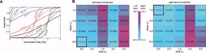
(A) Sigmoidal basis functions with the different shifts (κ) and slopes (η) employed in the gPLS analysis. Different colors in the figure indicate different shifts (κ). Different line styles in the figure indicate different slopes (η). Each analysis utilizes one sigmoidal basis function in addition to a constant and a linear basis function. (B) The cross validation error metrics ε calculated for different slopes (/η) and shifts (κ) during the gPLS analysis of left and right hand movement. The minimum error metric is marked with blue boundary box and blue text. The background color represents the linearly normalized value of the error metric ε. [Color figure can be viewed in the online issue, which is available at www.interscience.wiley.com.]

To quantify the marginal benefits of using sigmoidal basis functions, in addition to constant and linear ones, we began with a univariate general linear model (GLM) approach to regress the contrast images to obtain F‐statistic maps of task‐related activity [Friston et al., 1995]. In this process, we took a step‐wise approach that incorporated constant, linear, and sigmoidal functions into the GLM. We also derived a series of weights from empirical estimates of rate dependence measured in the contralateral primary motor areas (MI), and then used these weights as regressors to detect other active areas. We then compared the detection sensitivity among the different basis functions to determine which one yielded the maximum sensitivity in detecting the collection of regions exhibiting task‐related activity.

gPLS basis estimation using model cross validation

Given a dataset of specified size, multiple basis function choices can be made to fit the data with arbitrary precision. However, model fit usually increases at the cost of model complexity. The robustness of the model, defined here as the inverse of the discrepancy between model prediction and the left‐out observations, also decreases when the model becomes complicated. On the basis of the limited number of observations, we employ a “leave‐k‐out” cross validation scheme to test the robustness of the multivariate model. Basically, we randomly remove k observations, which are rows in the data matrix. With a chosen basis function, identified temporal LVs, singular values, and spatial LVs, the omitted observations can be used to generate cross validation data D _cv

(11)

, the difference between D _cv and the actual omitted rows of D, can be quantified using a sum‐of‐squares error metric, which is used as the goodness of fit in the model cross validation. Cross validation error is defined as the mean value of the root‐mean‐squares difference between D _cv and .

(12)

Here, denotes the Frobenius norm, the sum of squares of the matrix entries.

The cross validation error metric provides a quantitative assessment of the model robustness and allows selection among the model family members. Iterative random sampling of the data matrix along the observation dimension provides a stochastic measurement of both robustness and fit quality for linear models of various orders. Because of the computational efficiency of the gPLS algorithm, multiple realizations of the model can be explored in reasonable time. We then pool both model‐fitting and cross validation errors for each model.

In this article, we calculated 36 iterations to test the robustness of the spatiotemporal gPLS models. In each iteration, data from an individual participant at one movement rate (see Fig. 1) was reserved for cross validation. Then, the reduced data and the chosen basis functions were used to identify the spatiotemporal model [Eq. (8)], cross validation metrics ε, the square root of the Frobenius norm of the difference between the predicted data D _cv [Eq. (11)], and left‐out data , were then calculated over 36 iterations [Eq. (12)]. Average ε was used to estimate the crossvalidity of the model. In terms of robustness, those spatiotemporal models having minimal cross validation errors ε were considered optimal. We compared different models (sigmoidal basis functions with different slopes and shifts ) by calculating the average ε metric associated with each pair of and [Eq. (12)]. The model with minimal ε was considered to be optimal. The purpose of our cross validation procedure was to look for basis function parameters with both good model fit and robust performance across data subsets.

gPLS statistical inference

Given a selected basis function in gPLS analysis, the statistical significance of latent variables and the variability of significant brain LVs can be obtained using the nonparametric procedure proposed by McIntosh [McIntosh and Lobaugh, 2004; McIntosh et al., 1996a]. Specifically, two separate steps were used to estimate the variability of a specific latent variable and the distribution of the brain LV using a permutation test (sampling without replacement) and bootstrap (sampling with replacement), respectively. The permutation test was implemented to assess the variability of each LV by examining the fluctuation of singular values in the SVD, each iteration of which used a shuffled data matrix across different rows of D to estimate the variability of LVs in the null condition [McIntosh and Lobaugh, 2004]. Empirical P values of each LV were quantified as the ratio of the number of times where permuted data generated a higher singular value than the singular value from the original data over the total number of iterations. We ran 500 iterations of the permutation test. The variability of the spatial distribution of the effect loading was then estimated by the bootstrap procedure, which was repeated 500 times by random sampling data entry with replacement across different rows of D [McIntosh and Lobaugh, 2004]. The Z‐score of each image voxel was estimated from the ratio of the average pixel value and the standard deviation estimated across repeated bootstrap iterations.

Statistical tests of rate dependence

The distribution of the gPLS spatiotemporal model (a specified column of the basis function coefficients in matrix Φ) was estimated from the ensemble with a cross validation procedure.

(13)

To compare two models (specified columns in Φ₁ and Φ₂ respectively), we use the Hotelling's T ²‐statistic [Everitt and Dunn, 2001] .

(14)

Here, _i denotes the mean of the column i of the coefficient matrix. n ₁ and n ₂ are the numbers of cross validation iterations of the model. p represents the order of the basis, the number of entries in the coefficient vector _i, assuming both _i and _j are of identical order after padding necessary zero entries. Under the null hypothesis that the two coefficient vectors do not significantly differ, the distribution of T ² is given by:

(15)

To test whether the derived spatiotemporal model was independent, linearly dependent, or nonlinearly dependent on movement rate, we calculated various Hotelling's T ²‐statistics between columns of C and the associated P values [see Eqs. (14) and (15) and Appendix]. The optimal model identified with the cross validation procedure was compared with the constant basis (the zeroth‐order model), and the constant basis plus a linearly dependent basis (the first‐order model), to separately test whether the spatiotemporal models are independent or linearly dependent on movement rate for either hand.

Effective Connectivity Estimated With Structural Equation Modeling

The gPLS analysis revealed patterns of functional connectivity in our visuomotor experiment. Given the collection of identified active brain loci, we next estimated the directional influences among them using SEM.

Formulation of SEM

SEM is a mathematical tool using data covariance and correlations to reveal the strength of the directional modulation of neural ensembles. This method has been applied to the study of memory systems using PET data [McIntosh et al., 1994] and the attentional modulation of the visual system using fMRI data [Buchel and Friston, 1997]. SEM can reveal neural network dynamics during learning, attention, and working memory [Buchel et al., 1999; Friston and Buchel, 2000; McIntosh et al., 1996b]. Specifically, SEM needs two types of input data: one is the data covariance matrix among the brain areas of interest, and the other one is the directional connectivity graph among those regions. Subsequently, a numerical solver is used to derive estimates of the polarity and the strength of the directional influences as represented in the network directional connectivity graph. We used gPLS to identify the brain regions of interest and then calculated the data covariance matrix across subjects for each task condition. The section later describes the procedure we used to construct the directional connectivity graph. Next, we present the algorithm for estimating the paths in each task condition and then calculating the test statistics used to make inferences about the task‐related modulation of the corticocerebellar and corticostriatal loop activity.

SEM anatomical specification

The first step in the effective connectivity modeling procedure involved using the regions identified in the gPLS analysis to build a structural equation model. After thresholding the first dominant brain LV at the critical threshold that resulted in a similar volume of MI task‐related activity as in our previous study [Agnew et al., 2004], we identified the set of regions to include in the network analysis. As the permutation method we used to calculate the Z‐ scores in the gPLS procedure generally does not result in a normal distribution of values, special caution should be taken when selecting a Z‐score threshold for the purpose of obtaining physiologically reasonable functional brain LVs. In the present case, the justification for selecting a high‐calculated Z‐score is that we used the contrast images derived from task (movement) and the null (fixation) conditions in our gPLS analysis, instead of permuting between the task and the null conditions. Thus, we did not have observations that would allow direct estimation of the null condition variability. In addition, the effect space was limited to three degrees of freedom (from the three basis functions), resulting in low allowed variability.

Effective connectivity analysis using SEM requires an anatomical model with specified directional connections and unknown path values connecting the network nodes. We constructed an anatomical model with nodes derived from the gPLS analysis and internode connections derived from previous studies of primate neuroanatomy. The anatomical model we used has three main loops: a lateral corticocerebellar loop (ipsilateral cerebellum → contralateral thalamus → contralateral MI → ipsilateral cerebellum), a medial corticostriatal loop (contralateral SMA → putamen → globus pallidus → thalamus → SMA), and a lateral corticostriatal loop (contralateral MI → putamen → globus pallidus → thalamus → contralateral MI). A previous magnetoencephalography study of voluntary movement proposed a similar basic scheme of connectivity in the systems controlling voluntary movement [Gross et al., 2002].

In addition to an anatomical model, estimates of intrinsic activity variance at each node were calculated separately for observations from each movement rate and hand to obtain the endogenous source variance of each node in the network. In our calculation, we assumed that the intrinsic variance of each node was 50% of observed variance, as suggested in previous SEM studies [McIntosh and Gonzalez‐Lima, 1994; McIntosh et al., 1994].

SEM computation

The directional path coefficients were determined using SEM, based on the formulation developed by McArdle and McDonald [McArdle and McDonald, 1984],

(16)

where S denotes the endogenous source variance matrix between the nodes of the network, I is the identity matrix, and A is the path coefficient matrix with entry A_i,j at the ith row and the jth column quantifying the connection from node j to node i. The •^T superscript represents the transpose of the matrix. C represents the predicted covariance matrix among nodes in the network, which can be estimated from the time series as described earlier. To estimate the path coefficients, we adopted the maximal likelihood estimator, which minimizes the following cost function [Loehlin, 1998; McArdle and McDonald, 1984]:

(17)

where Tr[•] denotes the trace of the matrix, and det(•) denotes the determinant of a matrix; Φ represents the sample covariance matrix, and p is the number of paths in the anatomical model.

We used the nonlinear optimization tool from Matlab (Natick, MA) to search for the cost function minimum, repeating the estimation of path coefficients for 50 iterations, using a two‐sample bootstrap utilizing results from 12 participants. In this procedure, the datasets of two participants were replaced by data from two other participants, measured using the same hand and movement rates. Network analyses were then performed to test the rate dependency estimated by the gPLS procedure. Two different lateralized networks were explicitly tested: the corticocerebellar network consisting of ipsilateral cerebellum, contralateral thalamus, and contralateral MI; and the corticostriatal network consisting of contralateral MI, contralateral supplementary motor area (SMA), contralateral putamen/globus pallidus, and contralateral thalamus. To increase statistical power, all 50 iteratively calculated paths in each lateralized network were estimated to examine the correlations between the path coefficients and movement rate dependency (temporal scores shown in Fig. 4). For the analysis of lateralized hemispheric network activity, we excluded the callosal MI connections in order to decouple any possible interhemispheric interactions. A series of t tests were calculated to assess the statistical significance of the correlation between the path coefficients and the rate dependency of the network quantified by the temporal scores in the gPLS analysis.

Figure 4.

Relationship between movement rate and the temporal scores, which were calculated using [Eq. 9] after identifying the optimal model. Gray bars depict the standard deviation of recorded paced movement rates. In the group of right handed participants, signal modulation elicited by left hand movement demonstrates a more nonlinear rate dependence on movement frequency, while the right hand shows more linear rate dependence. Note that these curves represent the behavior across the entire LV. The dashed line represents an interval of one standard deviation estimated from 36 iterative cross validation analyses. [Color figure can be viewed in the online issue, which is available at www.interscience.wiley.com.]

RESULTS

Functional Connectivity Estimated With gPLS

Basis function parameter selection

We employed a range of transition slopes and shifts in the construction of the gPLS basis set, and the resulting basis functions are shown in Figure 2A. Specific combinations of transition slope and shift resulted in variations in overall model fit. Figure 2B shows the error metric (ε) calculated for different slopes () and shifts () and demonstrates that gPLS can be used to compare different parameter combinations selected from a basis function family with the same degrees of freedom. We identified the optimal parameters by choosing those associated with minimal cross validation error (ε). The slopes of the sigmoidal functions reflect saturation of the BOLD‐contrast signal as movement rate increases, whereas shifts of the sigmoidal functions indicate the threshold for movement rate modulation of activity. We found that sigmoidal functions with transition slope () 8 and shift () 0, in addition to constant and linear terms, were optimal for modeling the left‐hand data, whereas sigmoidal effects with transition slope () 1 and shift () 0, in addition to constant and linear terms, were optimal for modeling the right hand data.

Figure 3 shows the F‐statistic maps resulting from use of constant, linear, and sigmoidal functions to detect rate‐dependent activity. Notably, we found that the detection sensitivity increased from the constant, through the linear, to the sigmoidal function models. In relation to left hand movement, the SMA activation in medial premotor cortex was only detected by the linear and sigmoidal function models. Basal ganglia and contralateral MI activity were modeled with progressively increased sensitivity when we changed the basis functions from constant, through linear, to sigmoidal functions. Using the measured task‐related activity in contralateral MI as the regressor yielded weaker detection in the cerebellum and basal ganglia. In relation to left hand movement rate, the volume of detected voxels increased from 1,200 mm³ to 2,808 mm³ and finally to 2,976 mm³ (with the average t‐statistic growing from 3.611 to 4.11 and ultimately to 4.24) using constant, linear, and sigmoidal functions, respectively. Using the right hemisphere MI as the regressor gave a 2,224 mm³ active area and 4.75 average t‐statistic. Similarly, faster right hand movements were associated with a larger volumes of detected voxels, ranging from 664 mm³ to 1,736 mm³ and to 2,152 mm³, with the average t‐statistic growing from 3.28, to 3.79, and to 3.97. Using the left‐hemisphere MI as the regressor gave a 1,592 mm³ active area and a 3.81 average t‐statistic. Overall, the sigmoidal function provided the best detection sensitivity for the largest number of regions.

Figure 3.

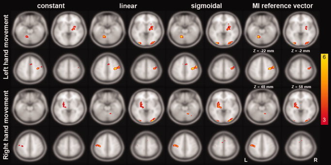
F‐statistic maps from a GLM analysis using constant, linear, and sigmoidal functions as regressors. In addition, to compare the detection sensitivity of this basis set to manual regressor identification methods, we also used a reference vector derived from an ROI surrounding the contralateral MI. The color scale represents the calculated F‐statistic. The critical threshold is P < 0.045, uncorrected. [Color figure can be viewed in the online issue, which is available at www.interscience.wiley.com.]

Latent variables

In the gPLS analysis, three LVs were calculated, corresponding to the three basis functions: constant, linear, and sigmoidal functions with specified slope and shift. We show the first LV, the most significant one, because of the relatively small effect space dimensionality. Spatiotemporal modeling using combinations of constant, linear, and sigmoidal functions with various shifts and transitions in leave‐one‐out cross validation identified different optimal models for right and left hand movements. The relative significance of the different LVs was quantified by the total variance in the effect space explained by each LV, which is equivalent to the ratio of the square of their singular values. The first LV of the optimal model for left and right hands captured 79% and 77% of the total variance and were statistically significant as evidenced by the results of the permutation test (P = 1.2% and 0.4% for left and right‐hand movements).

Rate dependence

Temporal scores describe the mapping between movement rate and normalized BOLD‐contrast signals, estimated using SVD to ensure that each temporal LV has unit variance. Figure 4 shows the temporal scores of the first LV in the identified optimal model. In that figure, the gray bars depict the actual movement rates in three major frequency ranges around 0.3, 1.0, and 3.0 Hz. The dashed lines in both the left and right hand models represent the standard deviation of the temporal model estimations resulting from 100 iterative computations. The first LV of the optimal model for the right hand indicates a more linear relationship between finger flexion rate and BOLD‐contrast signal around 0.3 to ∼2.0 Hz. The left hand optimal model shows a more nonlinear relationship between figure flexion rate and the BOLD‐contrast signal. The relationship tends to plateau above 0.7 Hz when the left hand is employed.

To characterize these responses as rate independent, linearly rate dependent or nonlinearly rate dependent, Hotelling's T ²‐statistics were used to examine effects of hand or movement rate in both the rate independent (constant) and the linearly rate dependent models. The Hotelling's T ²‐statistics comparing the left hand optimal model to the constant and linear models are 1.9 × 10⁸ and 8.0 × 10⁸, respectively, both of which have P values less than 10⁻⁴. Comparing the right hand optimal model to the constant and linear models gives T ²‐statistics of 4.0 × 10⁸ and 1.8 × 10⁸ (P < 0.01). These results show that the right‐hand first LV exhibits linear rate dependence, while the left hand first LV shows nonlinear rate dependence.

Spatial distribution of hand effects

The observed patterns of task‐related activity seen in the brain LVs changed reliably with respect to the hand used for the task. Figure 5 shows the spatial distribution of the brain LV Z‐scores thresholded between Z = 3 (uncorrected P = 0.1%) and Z = 6 (uncorrected P = 10⁻⁹).

Figure 5.

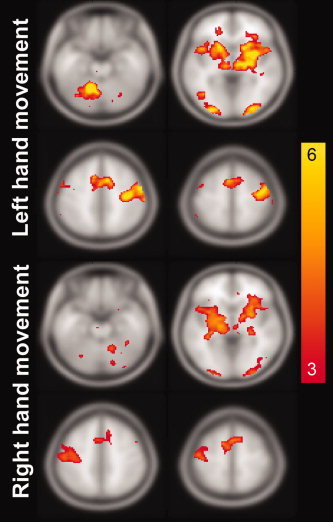
Active brain areas from the first brain LV resulting from the gPLS analysis for left (A) and right (B) hand movements using a Z‐score critical threshold of 45 (see text for details). The BOLD‐contrast responses in these areas show differential sensitivity to movement rate in the two hands, as shown in Figure 4. The units in these figures are the Z‐scores calculated from 100 iterative leave‐one‐out cross validations. The maps of Z‐scores transformed from correlation coefficients between movement rate and BOLD‐contrast signal are shown for left (C) and right (D) hand movements, using a critical threshold of Z > 2.0 (P < 0.023, uncorrected). The blue traces in (C) and (D) denote the borders of the active regions in the basal ganglia detected by the gPLS. [Color figure can be viewed in the online issue, which is available at www.interscience.wiley.com.]

The first brain LV related to right hand movement identified voxels in the ipsilateral cerebellum, bilateral visual cortex, contralateral thalamus, putamen, globus pallidus, primary, and SMAs, all regions exhibiting rate dependence, as seen by examining the first temporal scores (Fig. 5 bottom panel). For left hand movements, the first brain LV also identified the ipsilateral cerebellum, bilateral visual cortical areas, contralateral thalamus, putamen, globus pallidus, MI, and SMA, shown in the top panel of Figure 5. The MNI coordinates of local maxima comprising the first brain LVs for movements made with either hand are reported in Table I, along with the associated anatomical labels used in the subsequent SEM network analysis.

Table I.

Talairach coordinates, anatomical labels, and corresponding Brodmann area labels of the local maxima showing high sensitivity to movement rate in Figure 5A,B. (critical threshold Z‐score = 45 in the gPLS analysis)

SEM node	Anatomical label	Left hand movement					Right hand movement
		x	y	z	Volume (mm3)	BA	x	y	z	Volume (mm3)	BA
Cerebellum (LH)	Left cerebellum, anterior lobe	−15	−54	−19	112
	Left cerebellum, anterior lobe, culmen	−14	−53	−16	744
	Left cerebellum, posterior lobe, declive	−13	−58	−14	688
Cerebellum (RH)	Right cerebellum, anterior lobe						16	−52	−19	40
	Right cerebellum, anterior lobe, culmen						14	−52	−16	328
	Right cerebellum, posterior lobe, declive						13	−55	−13	72
Thalamus (LH)	Left brainstem, midbrain						−14	−18	−2	296
	Left Cerebrum, extranuclear						−18	−15	2	48
	Left cerebrum, thalamus						−14	−18	3	520
	Left cerebrum, sublobar, extranuclear						−18	−15	−2	40
Thalamus (RH)	Right brainstem, midbrain	15	−18	−1	144
	Right cerebrum, extra‐nuclear	18	−15	2	48
	Right cerebrum, thalamus	14	−17	3	504
	Right cerebrum, midbrain, extranuclear	18	−14	−1	8
	Right cerebrum, sublobar, thalamus	14	−17	6	168
Putamen/ Globus Pallidus (LH)	Left cerebrum, extranuclear						−19	−10	2	104
	Left cerebrum, lentiform nucleus						−25	−9	2	920
	Left cerebrum, sublobar, extranuclear						−28	−2	−4	568
	Left cerebrum, sublobar, lentiform nucleus						−24	−7	−2	816
Putamen/ Globus Pallidus (RH)	Right cerebrum, extranuclear	29	4	2	80
	Right cerebrum, lentiform nucleus	25	0	2	696
	Right cerebrum, sublobar, extra‐nuclear	27	9	−2	128
	Right cerebrum, sublobar, lentiform nucleus	25	3	0	512
MI (LH)	Left cerebrum, frontal lobe, postcentral gyrus						−44	−16	44	64
	Left cerebrum, frontal lobe, precentral gyrus						−44	−13	45	832	4
	Left cerebrum, frontal lobe, subgyral						−33	−19	41	48
	Left cerebrum, parietal lobe, postcentral gyrus						−48	−15	45	488	[1 3]
	Left cerebrum, parietal lobe, precentral gyrus						−50	−14	39	8	4
MI (RH)	Right cerebrum, frontal lobe, postcentral gyrus	53	−10	45	64
	Right cerebrum, frontal lobe, precentral gyrus	52	−7	43	448	[4 6]
	Right cerebrum, parietal lobe, postcentral gyrus	54	−11	45	24	3
SMA (LH)	Left cerebrum, frontal lobe, medial frontal gyrus	−4	6	49	184	[6 32]	−5	3	50	136	6
	Left cerebrum, frontal lobe, superior frontal gyrus	−3	8	51	184	6	−4	6	51	80	6
	Left cerebrum, limbic lobe, cingulate gyrus	−2	3	46	16	24
SMA (RH)	Right cerebrum, frontal lobe, medial frontal gyrus	5	9	46	456	[6 32]	6	12	47	80	[6 32]
	Right cerebrum, frontal lobe, superior frontal gyrus	5	12	50	312	6	5	14	51	408	[6 8]
	Right cerebrum, limbic lobe, cingulate gyrus	6	8	43	64	[24 32]

Regional BOLD‐contrast signal changes are shown in Figure 6, where we separated the regions detected by the gPLS technique into two lateralized subsystems containing ipsilateral cerebellum and contralateral MI, globus pallidus, putamen, thalamus, and SMA. Cerebral areas contralateral and cerebellar areas ipsilateral to the moving hand showed larger task‐related modulation. Also, in general, BOLD‐contrast signals increased with movement rate.

Figure 6.

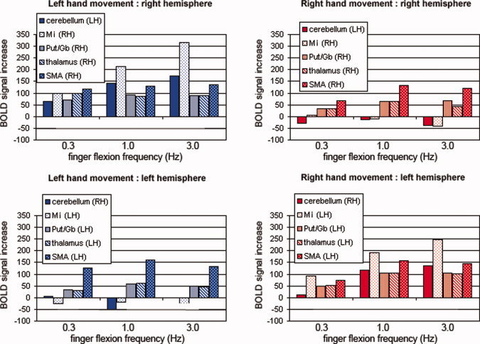
Region‐of‐interest (ROI) measurements of BOLD‐contrast movement minus fixation signals revealed by the gPLS technique for left and right hand movements at 0.3, 1.0, and 3.0 Hz. ROIs were identified by thresholding the first dominant brain LV in the gPLS analysis with Z‐scores higher than 45. For this analysis, the brain areas were separated into lateralized corticocerebellar and corticostriate systems containing ipsilateral cerebellum and contralateral MI, putamen, globus pallidus, SMA, and thalamus. [Color figure can be viewed in the online issue, which is available at www.interscience.wiley.com.]

Effective Connectivity Estimated With SEM

To model rate‐dependent modulation of effective connectivity in the systems controlling hand movement, the previous behavioral data‐driven gPLS modeling results were used to specify the coordinates of the functionally specialized “nodes.” Model regions included the bilateral cerebellar hemispheres, thalamus, putamen, globus pallidus, supplementary, and primary motor areas. Although there was significant task‐related modulation seen in the visual system, these areas were not included in the SEM model because of the attendant complexity that their inclusion would add to the overall analysis, as additional paths would be required to represent the connections those areas make with various parts of the motor system.

The values of effective connectivity estimated by SEM are reported in Table II for hand movements performed at varying rates. Figure 7 illustrates the effective connectivity pattern after thresholding the values at a Z‐score of 0.6745 (two‐tailed test uncorrected P value = 0.5), where red arrows indicate positive path coefficients, and blue arrows represent negative path coefficients. The width of each arrow corresponds to the path value. The reason for choosing such a generous critical threshold was to allow examination of activity in the highest number of paths specified in the anatomical component of the model. This constraint also reflects the limited number of participants in this study, and we expect that a more stringent threshold could be used with a larger sample. Similar low thresholds for path coefficient maps have been previously reported in a bimanual movement fMRI SEM study [Zhuang et al., 2005]. Paths with absolute Z‐scores less than 0.6745 are gray in color to indicate their lack of statistical significance.

Table II.

Path coefficient averages and standard deviations from 50 iterative structural equation modeling calculations

Path		Left hand; 0.3 Hz	Right hand; 0.3 Hz	Left hand; 1 Hz	Right hand; 1 Hz	Left hand; 3 Hz	Right hand; 3 Hz
From	To
Cerebellum (LH)	Thalamus (RH)	0.61 (0.75)*	0.13 (0.31)	0.68 (0.33)*	−0.06 (0.68)	0.22 (0.24)*	0.43 (0.60)*
Cerebellum (RH)	Thalamus (LH)	−0.21 (0.20)*	0.23 (0.25)*	−0.11 (0.28)	−0.03 (1.33)	0.12 (0.44)	0.15 (0.31)
Thalamus (RH)	SMA (RH)	0.94 (0.25)*	1.20 (0.59)*	1.00 (0.26)*	1.20 (0.70)*	1.25 (0.74)*	1.62 (0.96)*
Thalamus (LH)	SMA (LH)	1.97 (0.56)*	0.87 (0.59)*	1.99 (0.58)*	1.30 (0.61)*	2.00 (1.07)*	1.29 (0.49)*
MI (LH)	MI (RH)	−0.33 (0.65)	0.13 (0.42)	0.80 (0.55)*	−0.32 (0.66)*	1.09 (1.93)	−0.52 (0.58)*
MI (RH)	MI (LH)	0.15 (0.68)	0.54 (0.27)*	0.15 (0.36)	−0.39 (0.75)	0.08 (0.41)	0.27 (0.76)
SMA (LH)	MI (LH)	−0.34 (0.59)	0.53 (0.24)*	−0.06 (0.43)	0.56 (0.63)*	0.09 (0.75)	0.53 (0.69)*
SMA (RH)	MI (RH)	0.35 (0.40)*	0.01 (0.38)	0.90 (0.42)*	0.49 (0.69)*	0.32 (1.11)	0.95 (0.85)*
MI (RH)	Cerebellum (LH)	0.51 (0.12)*	−0.21 (0.41)	0.50 (0.12)*	0.27 (0.14)*	0.49 (0.03)*	0.31 (0.19)*
MI (LH)	Cerebellum (RH)	0.03 (0.36)	0.00 (0.24)	0.46 (0.24)*	0.53 (0.10)*	0.88 (0.51)*	0.48 (0.11)*
Thalamus (LH)	MI (LH)	0.32 (0.44)*	0.70 (0.33)*	−0.61 (0.51)*	0.90 (1.02)*	−1.13 (0.85)*	1.45 (1.10)*
Thalamus (RH)	MI (RH)	0.16 (0.44)	−0.60 (0.74)*	0.95 (0.74)*	−0.00 (0.52)	3.04 (2.34)*	−0.48 (1.05)
SMA (LH)	Putamen/Globus pallidus (LH)	0.16 (0.16)*	0.31 (0.21)*	0.32 (0.17)*	0.25 (0.20)*	0.26 (0.12)*	0.06 (0.17)
SMA (RH)	Putamen/Globus pallidus (RH)	0.33 (0.25)*	0.38 (0.25)*	0.41 (0.14)*	0.32 (0.13)*	0.21 (0.17)*	0.48 (0.09)*
Putamen/globus pallidus (LH)	Thalamus (LH)	1.16 (0.46)*	0.77 (0.22)*	0.93 (0.33)*	0.95 (1.47)	1.02 (0.43)*	0.72 (0.34)*
Putamen/globus pallidus (RH)	Thalamus (RH)	0.74 (0.77)*	0.61 (0.46)*	−0.14 (0.40)	0.99 (0.41)*	0.47 (0.42)*	0.41 (0.52)*
MI (LH)	Putamen/globus pallidus (LH)	0.17 (0.40)	0.12 (0.28)	0.27 (0.61)	0.28 (0.19)*	−0.17 (0.29)	0.31 (0.13)*
MI (RH)	Putamen/globus pallidus (RH)	0.27 (0.19)*	0.12 (0.45)	0.20 (0.08)*	−0.15 (0.28)	0.14 (0.09)*	−0.09 (0.16)

^*Statistically significant paths (absolute Z‐scores < 0.6745, two‐tail uncorrected P < 0.5).

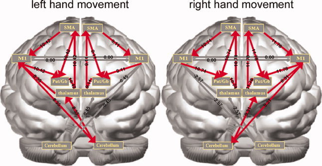
Figure 7.

The path coefficients for visually paced variable‐rate movements of the left (left column) and right (right column) hands. Top: 0.3 Hz; Middle: 1.0 Hz; Bottom: 3.0 Hz. The widths of the arrows correspond to the magnitude of the estimated path coefficients, which are also noted directly above the arrows. Red arrows represent positive path coefficients, and blue arrows represent negative path coefficients. Arrows with absolute Z‐scores > 0.6745 (two‐tail uncorrected p < 0.5) are plotted in gray. The brain is shown from the front with the left hemisphere on the right of the figure. [Color figure can be viewed in the online issue, which is available at www.interscience.wiley.com.]

Effective connectivity during the slowest movements

During low‐frequency (∼0.3 Hz) movements of the left hand, the major positive active connections were from left cerebellum to right thalamus, with an estimated path coefficient of 0.61, and from right MI to left cerebellum, with a path coefficient of 0.51. The path coefficients in the corticostriatal loop in both hemispheres were also positive. Stronger interactions might be expected with tasks involving intermanual coordination. Note that negative effective connectivity was observed from right cerebellum to left thalamus during left hand movement at 0.3 Hz. For right hand movements executed at the same 0.3 Hz frequency, active connections were detected from right cerebellum to left thalamus and then to left MI, with estimated path coefficients of 0.23 and 0.70, respectively. The medial corticostriatal loops in both hemispheres exhibited positive, statistically significant effects. One statistically significant negative influence from thalamus to MI of the right hemisphere was observed.

Effective connectivity during intermediate speed movements

During the 1.0 Hz left hand movements, the effective connectivity of the lateral corticocerebellar loop was positive. We also estimated positive right SMA‐>right MI effective connectivity and positive right SMA‐>right putamen/globus pallidus connectivity. The connectivity from right SMA to right MI was statistically significant (path coefficient = 0.90). For right hand 1.0 Hz movement, although the ipsilateral cerebellum‐>contralateral thalamus connectivity was statistically insignificant, the contralateral thalamus‐>MI connectivity was positive and stronger than in the 0.3 Hz condition. The connectivity from contralateral MI to ipsilateral cerebellum was significantly positive. The effective connectivity from contralateral thalamus to SMA, and from contralateral SMA to contralateral putamen/globus pallidus were both positive and the SMA‐>MI connectivity was significantly positive in both hemispheres.

Effective connectivity during the fastest movements

Effective connectivity associated with 3.0 Hz left hand movement was remarkable for the following positive paths: left cerebellum to right thalamus (0.22), right thalamus to right MI (3.04), and right MI to left cerebellum (0.49). The paths in the medial corticostriatal loop in both the left and right hemispheres were all positive. Note that significant negative effective connectivity was also estimated from left thalamus to left MI (−1.13). Right hand movement at 3.0 Hz was associated with positive effective connectivity paths: from right cerebellum to left thalamus (0.15; not statistically significant), from left thalamus to left MI (1.45), and from right MI to left cerebellum (0.48). Both hemispheres showed strong positive thalamus‐>SMA connectivity. The connectivity from SMA‐>MI was significantly positive in both hemispheres.

Corticocerebellar vs. corticostriate effects

To investigate the modulations in effective connectivity with respect to manual specialization in the two lateralized hemispheric networks involved in visuomotor control, we separately modeled left and right hand movements using regression analysis. For left hand movements performed at 0.3 Hz, 1.0 Hz, and 3.0 Hz, the regression vectors were [0.10, 0.18, 0.18]. For right hand movements at 0.3 Hz, 1.0 Hz, and 3.0 Hz, the regression vectors were [0.10, 0.16, 0.22]. These values were similar to the pattern seen in the temporal scores in the gPLS analysis (see Fig. 4). Figure 8 shows the t‐statistics resulting from regression coefficient testing the null hypothesis that the coefficient for the regression vector is zero. When the network paths were thresholded at t = 7.0 (P value < 0.0001 uncorrected), we found that, when switching between left and right hand movements, the lateralized corticocerebellar network switched between hemispheres and showed rate dependence, as revealed by the gPLS procedure. In contrast, the effective connectivity among the regions comprising the corticostriatal networks in each hemisphere showed rate dependence revealed by the gPLS procedure that did not appear to differ with respect to hand. These results demonstrate the ability of combined functional and effective connectivity analysis to capture the influence of behavioral context on the interregional influences among the cortical motor system components and their subcortical targets.

Figure 8.

The t‐statistics from the regression analysis using temporal scores shown in Figure 4 to regress path coefficients during left and right hand movement. Note that the lateralized corticocerebellar network switched with respect to hand. Both lateralized corticostriatal networks show statistically significant symmetric movement rate dependence. Statistically significant paths are shown in red (critical threshold at t = 7.0, p < 0.0001, uncorrected). [Color figure can be viewed in the online issue, which is available at www.interscience.wiley.com.]

DISCUSSION

gPLS Functional Connectivity and SEM Effective Connectivity Methods

We combined functional and effective connectivity estimation procedures in a novel two‐stage network analysis to reveal hemispheric specialization of the neural systems responsible for controlling variable‐rate, visually paced, finger movements. The integrated method captured the strong modulations in activity that can be seen when hand use is varied along with parametric variations in movement rate. Our modeling strategy combined gPLS methods [Lin et al., 2003; McIntosh et al., 1996a], which identified nodes in spatially distributed networks, with subsequent SEM, allowing estimation of the effective connectivity between the previously identified nodes. Similar to PLS, gPLS analyzes the covariance matrix between the neuroimaging data and the experimental design in a multivariate framework. In addition, gPLS covaries basis functions parameterized by behavioral measures with fMRI time series to create a space accounting for the correlations between brain regions exhibiting signal modulations with respect to effects or task variables of interest. Thus, gPLS successfully revealed functional connectivity related to performance of a simple visuomotor task, indicating the utility of this multivariate modeling technique in identifying functionally coherent activity patterns without prior anatomical information. In contrast to the previous studies that have demonstrated regionally specific relationships between movement rate and neural activity, our approach additionally identified the interactions among distributed brain regions and their behavioral correlates. However, gPLS analysis alone does not address directional influences among participating regionally specialized brain structures. For this reason, we subsequently used SEM for effective connectivity analysis, as it can allow estimation of directional effects among regions. Results from the combination of gPLS and SEM provide general spatiotemporal descriptions of the systems responsible for the orchestration of perception and action modeled at the system level.

The principal novelty of our two‐stage analysis procedure relies on the use of robust multivariate linear modeling to decompose the partial covariance matrix between behavioral measurements and neuroimaging time series. Conventionally, multivariate analysis of functional images has combined principle component analysis (PCA) and canonical variate analysis (CVA) [Friston et al., 1995]. Another multivariate technique, PLS [McIntosh et al., 1996a], uses PCA to dissect the projection of functional data into multiple contrasts of interest. Compared with multivariate techniques that directly analyze the structural variance within functional images, the advantages of PLS include the ability to make simultaneous multiple contrast comparisons, superior computational efficiency, and simplified procedures for post hoc interpretation of the decomposed data structures. These advantages all derive from the decomposition of collapsed effects into the orthogonal subspaces that are constrained mathematically using PCA. Alternative constraints have also been suggested to minimize mutual information among the decomposed components using independent component analysis [Bell and Sejnowski, 1995; McIntosh et al., 1998; McKeown et al., 1998]. We recently proposed the use of either PCA or ICA for data decomposition in gPLS procedures [Lin et al., 2003]. In time series analysis, gPLS is capable of detecting both transient and consistent activities by randomly categorizing repetitive observations into groups. Additionally, this randomized grouping approach can assess the robustness of the decomposed components. However, problems related to selecting the appropriate randomized grouping number have not been previously resolved. In this article, we employed cross validation to determine the optimal parameters of the brain model. The same principle may be usefully applied to select the optimal randomized grouping number in the analysis of time series data. Given finite data samples, it is possible to test the robustness of the optimal model by using “leave‐one‐out” cross validation.

In all gPLS modeling implementations, basis functions are required for identification. In theory, we have no preference for any specific basis function set, as long as those in the model are capable of capturing the essential features present in the data. This means that the chosen basis functions should fully span the effect space constructed by correlating neuroimaging and behavioral measurements. For this purpose, either discrete or continuous basis functions are feasible alternatives. In the present context, our aim was to relate continuous external behavior measurements (finger movement rate) to brain activity. A previous study employing a similar parametric experimental design but using mass univariate modeling techniques, showed that either a linearly rate‐dependent model or step function models can best fit different brain areas [VanMeter et al., 1995]. The sigmoidal basis functions with parametrically varying shifts and transitions we employed allowed exploration of a model ranging between linear rate dependence and a step function to better characterize the brain BOLD‐contrast responses observed in relation to variable‐rate movements. As shown by the gPLS results, differential behavior/BOLD‐contrast responses could be identified automatically with respect to dominant versus nondominant hand movements without resorting to laborious manual specification of the MRI signal dependence on the kinematic properties of the movements. The present results approximated those seen in our previous study which utilized a mass univariate modeling technique to characterize parametric rate modulation of brain activity [Agnew et al., 2004]. The current approach is especially suitable for parametrically designed fMRI experiments as it provides an efficient means to automatically interrogate the quantitative relationship between neural activity patterns and behavior. There may be a need to tailor basis function selection to particular study characteristics and a judicious choice of basis functions may be achieved by using prior physiological and mathematical information in order to avoid high‐dimensional parameter spaces, obtain computationally efficient parameter identification, and allow physiologically sensible inferences.

Overall, the gPLS method we describe differs from standard PLS analysis methods [McIntosh and Lobaugh, 2004; McIntosh et al., 1996a] in the two aspects. First, basis functions are introduced to transform the behavioral measurements into models, which are then crosscorrelated with the neuroimaging data to construct the effect space. Second, a cross validation procedure is used to achieve simultaneous identification of the optimal parameters for the basis functions and establish the robust performance of the model.

Motor System Property Identification

Using combined gPLS and SEM, we successfully characterized the functional anatomy of the visuomotor system under conditions of varying paced movement rate. The motor control networks identified confirmed those seen in previous neuroimaging studies that found a rate‐dependent system consisting of contralateral primary motor, contralateral thalamus and ipsilateral cerebellum [Blinkenberg et al., 1996; Jancke et al., 1998; Khushu et al., 2001; Rao et al., 1996; Sadato et al., 1996a, b, 1997; Schlaug et al., 1996; Turner et al., 1998; VanMeter et al., 1995]. In our study, visual cortical areas showed strong rate dependence, undoubtedly due to the variable‐rate visual cues used to pace the movements [Fox and Raichle, 1984].

At different rates, this spatially distributed visuomotor control system works in an orchestrated fashion to control both right and left hand movement, exhibiting integrated modulation of the effective connectivity among its constituent specialized processing areas. The gPLS procedure identified one LV from which two networks were defined with reference to the existing literature on motor system connectivity patterns. The observed linearly rate‐dependent characteristic of right hand movements between 0.3 Hz and 2.0 Hz agrees with previous SPECT [Sabatini et al., 1993], PET [Sadato et al., 1996a; VanMeter et al., 1995], and fMRI findings [Rao et al., 1996; Sadato et al., 1997; Schlaug et al., 1996]. The left hand movements were associated with nonlinearly rate‐dependent activity, with increasing responses from 0.3 Hz to about 1.0 Hz and a very slow increase with the movement rate between 1.0 Hz and 3.0 Hz. Expanding the system characterization possible with traditional mass univariate modeling, our gPLS approach identified the patterns of functional and effective connectivity associated with executing a simple visuomotor task, demonstrating that, whereas bilateral primary motor, SMAs, thalamus, putamen, and globus pallidus, as well as cerebellum hemispheres, are all involved in controlling movement of either hand, they are differentially engaged during left and right hand use. The demonstration of differential rate dependence between left and right hand movements supports a model of hemispheric asymmetry for the control of voluntary movement, in agreement with previous anatomical [Amunts et al., 1996] and functional [Agnew et al., 2004; Dassonville et al., 1997] findings. This asymmetric pattern of effective connectivity may be related to either the differential manual experience or the biologically determined manual preference which characterized our sample group of strongly right handed participants. Further studies with participants exhibiting a more balanced or left manual preference will be required to investigate these alternative origins for the observed hemispheric asymmetries in visuomotor system organization.

The use of SEM resulted in several interesting findings. First, the lateralized corticocerebellar motor loop exhibited stronger positive modulation as movement rate increased. This finding is consistent with previous univariate modeling analyses [Sadato et al., 1996a, b; VanMeter et al., 1995] that showed stronger MI and cerebellum activity at higher movement rates. A recent SEM study also reported similar hemispherically lateralized organization of the motor system [Taniwaki et al., 2006]. However, our results demonstrated an addition shift of lateralization of movement rate‐dependent corticocerebellar loop activity when the participants used either hand. In addition, we were able to select regions of interest for the SEM analysis via the relatively automatic multivariate gPLS approach, avoiding the standard type of mass univariate analysis that neglects spatial correlation in the process of identifying sets of functionally active visuomotor areas. Our SEM results showed that, at low movement rates, strong effective connectivity was seen in the connection from the ipsilateral cerebellum to the contralateral thalamus, whereas at higher movement rates, the effective connectivity from contralateral thalamus to contralateral MI was found to be dominant. Second, the medial corticostriatal loop was consistently active across the three movement rates using either hand, showing a lack of modulation of the corticostriatal system with respect to movement rate. Interestingly, the connectivity in this corticostriatal circuit is mostly positively modulated, except in the contralateral putamen/globus pallidus‐thalamus connection for 1 Hz movement rates. Third, the SMA to MI path demonstrated differential rate effective connectivity with movements of either hand. Using the left hand, the contralateral SMA to MI effective connectivity was strong only during low rates of movement, whereas when using the right hand, SMA to MI effective connectivity in both hemispheres was high. Lastly, the negative modulation seen in connections to the ipsilateral MI area is in agreement with recent reports of task‐related deactivation patterns [Allison et al., 2000; Nirkko et al., 2001; Reddy et al., 2000]. The observed suppression of the ipsilateral primary motor area might be from either ipsilateral thalamus or contralateral MI, as shown in the SEM results in our experiment. These significant negative modulations are consistent with the suggestion that these connections may be responsible for suppression of mirror movements [Nirkko et al., 2001; Reddy et al., 2000].

The SEM analysis also revealed that the cerebellar hemispheres participated in paced movement with distinct patterns. First, we found that the cerebellar activity is rate dependent. Second, through effective connectivity analysis, we found that changes in effective connectivity to and from the cerebellum associated with movement kinematics, specifically rate changes. This finding is also in agreement with the general suggestion that the cerebellum has a significant role in sensorimotor integration, possibly monitoring the sensory consequences of movement [Gao et al., 1996].

Network analysis of the functional organization of the human sensorimotor system has potential applicability to the characterization of the processes responsible for manual dominance. Because handedness is presumably derived from long‐term skill acquisition built on a genetically determined functional and anatomic infrastructure—a topic still under debate [Amunts et al., 1996; White et al., 1997]—we expect that learning and experience might alter both the functional and effective connectivity of the specialized processing regions comprising the motor system. A specific example is the recent work reporting modification of effective connectivity through visuomotor learning [Toni et al., 2002]. We speculate that via motor learning the rate dependency revealed by gPLS and the asymmetry of the hemispheric networks identified by SEM may change over time. In clinical applications, it is possible that the two‐stage modeling procedure that we introduce in this article could reveal differential motor system responses when contrasting typical participants to those with lesions affecting specific motor system components, as it has recently been shown that patients with Parkinson's disease exhibited characteristically enhanced attentional modulation of effective connectivity between the SMA and premotor cortical areas [Rowe et al., 2002]. Spatiotemporal modeling utilizing combined estimates of functional and effective connectivity may be useful for characterizing the functional organization of the sensorimotor system in various clinical contexts.

HOTELLING's T2 STATISTICS

Hotelling's T ² is a generalized t‐test used for multivariate hypothesis testing [Hotelling, 1931]. Specifically, we can test the null hypothesis that two vector x and y are identical:

The Hotelling's T ² statistics is:

(A1)

Then, T ² statistic can be related to the F‐distribution as

(A2)

REFERENCES

- Agnew JA,Zeffiro TA,Eden GF ( 2004): Left hemisphere specialization for the control of voluntary movement rate. Neuroimage 22: 289–303. [DOI] [PubMed] [Google Scholar]
- Allison JD,Meador KJ,Loring DW,Figueroa RE,Wright JC ( 2000): Functional MRI cerebral activation and deactivation during finger movement. Neurology 54: 135–142. [DOI] [PubMed] [Google Scholar]
- Amunts K,Schlaug G,Schleicher A,Steinmetz H,Dabringhaus A,Roland PE,Zilles K ( 1996): Asymmetry in the human motor cortex and handedness. Neuroimage 4: 216–222. [DOI] [PubMed] [Google Scholar]
- Bell AJ,Sejnowski TJ ( 1995): An information‐maximization approach to blind separation and blind deconvolution. Neural Comput 7: 1129–1159. [DOI] [PubMed] [Google Scholar]
- Blinkenberg M,Bonde C,Holm S,Svarer C,Andersen J,Paulson OB,Law I ( 1996): Rate dependence of regional cerebral activation during performance of a repetitive motor task: A PET study. J Cereb Blood Flow Metab 16: 794–803. [DOI] [PubMed] [Google Scholar]
- Buchel C,Friston KJ ( 1997): Modulation of connectivity in visual pathways by attention: Cortical interactions evaluated with structural equation modelling and fMRI. Cereb Cortex 7: 768–778. [DOI] [PubMed] [Google Scholar]
- Buchel C,Coull JT,Friston KJ ( 1999): The predictive value of changes in effective connectivity for human learning. Science 283: 1538–1541. [DOI] [PubMed] [Google Scholar]
- Colebatch JG,Deiber MP,Passingham RE,Friston KJ,Frackowiak RS ( 1991): Regional cerebral blood flow during voluntary arm and hand movements in human subjects. J Neurophysiol 65: 1392–1401. [DOI] [PubMed] [Google Scholar]
- Dassonville P,Zhu XH,Uurbil K,Kim SG,Ashe J ( 1997): Functional activation in motor cortex reflects the direction and the degree of handedness. Proc Natl Acad Sci USA 94: 14015–14018. [DOI] [PMC free article] [PubMed] [Google Scholar]
- Everitt B,Dunn G ( 2001):Applied Multivariate Data Analysis, Vol. x London: Arnold, 342 p. [Google Scholar]
- Fox PT,Raichle ME ( 1984): Stimulus rate dependence of regional cerebral blood flow in human striate cortex, demonstrated by positron emission tomography. J Neurophysiol 51: 1109–1120. [DOI] [PubMed] [Google Scholar]
- Fox PT,Fox JM,Raichle ME,Burde RM ( 1985): The role of cerebral cortex in the generation of voluntary saccades: A positron emission tomographic study. J Neurophysiol 54: 348–369. [DOI] [PubMed] [Google Scholar]
- Friston KJ,Buchel C ( 2000): Attentional modulation of effective connectivity from V2 to V5/MT in humans. Proc Natl Acad Sci USA 97: 7591–7596. [DOI] [PMC free article] [PubMed] [Google Scholar]
- Friston KJ,Frith CD,Liddle PF,Frackowiak RS ( 1993): Functional connectivity: The principal‐component analysis of large (PET) data sets. J Cereb Blood Flow Metab 13: 5–14. [DOI] [PubMed] [Google Scholar]
- Friston KJ,Holmes AP,Poline JB,Grasby PJ,Williams SC,Frackowiak RS,Turner R ( 1995): Analysis of fMRI time‐series revisited. Neuroimage 2: 45–53. [DOI] [PubMed] [Google Scholar]
- Friston KJ,Buechel C,Fink GR,Morris J,Rolls E,Dolan RJ ( 1997): Psychophysiological and modulatory interactions in neuroimaging. Neuroimage 6: 218–229. [DOI] [PubMed] [Google Scholar]
- Gao JH,Parsons LM,Bower JM,Xiong J,Li J,Fox PT ( 1996): Cerebellum implicated in sensory acquisition and discrimination rather than motor control. Science 272: 545–547. [DOI] [PubMed] [Google Scholar]
- Grafton ST,Mazziotta JC,Woods RP,Phelps ME ( 1992): Human functional anatomy of visually guided finger movements. Brain 115(Part 2): 565–587. [DOI] [PubMed] [Google Scholar]
- Gross J,Timmermann L,Kujala J,Dirks M,Schmitz F,Salmelin R,Schnitzler A ( 2002): The neural basis of intermittent motor control in humans. Proc Natl Acad Sci USA 99: 2299–2302. [DOI] [PMC free article] [PubMed] [Google Scholar]
- Hotelling H ( 1931): The generalization of Student's ratio. Ann Math Statist 2: 360–378. [Google Scholar]
- Jancke L,Specht K,Mirzazade S,Loose R,Himmelbach M,Lutz K,Shah NJ ( 1998): A parametric analysis of the ‘rate effect’ in the sensorimotor cortex: A functional magnetic resonance imaging analysis in human subjects. Neurosci Lett 252: 37–40. [DOI] [PubMed] [Google Scholar]
- Kandel ER,Schwartz JH,Jessell TM ( 2000):Principles of Neural Science, Vol. xli New York: McGraw‐Hill Health Professions Division; 1414 p. [Google Scholar]
- Khushu S,Kumaran SS,Tripathi RP,Gupta A,Jain PC,Jain V ( 2001): Functional magnetic resonance imaging of the primary motor cortex in humans: Response to increased functional demands. J Biosci 26: 205–215. [DOI] [PubMed] [Google Scholar]
- Le Bihan D,Karni A ( 1995): Applications of magnetic resonance imaging to the study of human brain function. Curr Opin Neurobiol 5: 231–237. [DOI] [PubMed] [Google Scholar]
- Lin FH,McIntosh AR,Agnew JA,Eden GF,Zeffiro TA,Belliveau JW ( 2003): Multivariate analysis of neuronal interactions in the generalized partial least squares framework: Simulations and empirical studies. NeuroImage 20: 625–642. [DOI] [PubMed] [Google Scholar]
- Loehlin JC ( 1998):Latent Variable Models: An Introduction to Factor,Path, and Structural Analysis, Vol. xi Mahwah, NJ: Lawrence Erlbaum; 309 p. [Google Scholar]
- McArdle JJ,McDonald RP ( 1984): Some algebraic properties of the Reticular Action Model for moment structures. Br J Math Stat Psychol 37(Part 2): 234–251. [DOI] [PubMed] [Google Scholar]
- McIntosh AR,Gonzalez‐Lima F ( 1994): Network interactions among limbic cortices, basal forebrain, and cerebellum differentiate a tone conditioned as a Pavlovian excitor or inhibitor: Fluorodeoxyglucose mapping and covariance structural modeling. J Neurophysiol 72: 1717–1733. [DOI] [PubMed] [Google Scholar]
- McIntosh AR,Lobaugh NJ ( 2004): Partial least squares analysis of neuroimaging data: Applications and advances. Neuroimage 23 ( Suppl 1): S250–S263. [DOI] [PubMed] [Google Scholar]
- McIntosh AR,Grady CL,Ungerleider LG,Haxby JV,Rapoport SI,Horwitz B ( 1994): Network analysis of cortical visual pathways mapped with PET. J Neurosci 14: 655–666. [DOI] [PMC free article] [PubMed] [Google Scholar]
- McIntosh AR,Bookstein FL,Haxby JV,Grady CL ( 1996a): Spatial pattern analysis of functional brain images using partial least squares. Neuroimage 3: 143–157. [DOI] [PubMed] [Google Scholar]
- McIntosh AR,Grady CL,Haxby JV,Ungerleider LG,Horwitz B ( 1996b): Changes in limbic and prefrontal functional interactions in a working memory task for faces. Cereb Cortex 6: 571–584. [DOI] [PubMed] [Google Scholar]
- McIntosh AR,Lobaugh NJ,Cabeza R,Bookstein FL,Houle S ( 1998): Convergence of neural systems processing stimulus associations and coordinating motor responses. Cereb Cortex 8: 648–659. [DOI] [PubMed] [Google Scholar]
- McKeown MJ,Makeig S,Brown GG,Jung TP,Kindermann SS,Bell AJ,Sejnowski TJ ( 1998): Analysis of fMRI data by blind separation into independent spatial components. Hum Brain Mapp 6: 160–188. [DOI] [PMC free article] [PubMed] [Google Scholar]
- Nirkko AC,Ozdoba C,Redmond SM,Burki M,Schroth G,Hess CW,Wiesendanger M ( 2001): Different ipsilateral representations for distal and proximal movements in the sensorimotor cortex: Activation and deactivation patterns. Neuroimage 13: 825–835. [DOI] [PubMed] [Google Scholar]
- Nolte J ( 1998):The Human Brain: An Introduction to Its Functional Anatomy, Vol. xi St. Louis, MO: Mosby; 606p. [Google Scholar]
- Oldfield RC ( 1971): The assessment and analysis of handedness: The Edinburgh inventory. Neuropsychologia 9: 97–113. [DOI] [PubMed] [Google Scholar]
- Rao SM, Binder JR, Bandettini PA, Hammeke TA, Yetkin FZ, Jesmanowicz A, Lisk LM, Morris GL, Mueller WM, Estkowski LD, Wong EC, Haughton VM, Hyde JS ( 1993): Functional magnetic resonance imaging of complex human movements. Neurology 43: 2311–2318. [DOI] [PubMed] [Google Scholar]
- Rao SM,Binder JR,Hammeke TA,Bandettini PA,Bobholz JA,Frost JA,Myklebust BM,Jacobson RD,Hyde JS ( 1995): Somatotopic mapping of the human primary motor cortex with functional magnetic resonance imaging. Neurology 45: 919–924. [DOI] [PubMed] [Google Scholar]
- Rao SM,Bandettini PA,Binder JR,Bobholz JA,Hammeke TA,Stein EA,Hyde JS ( 1996): Relationship between finger movement rate and functional magnetic resonance signal change in human primary motor cortex. J Cereb Blood Flow Metab 16: 1250–1254. [DOI] [PubMed] [Google Scholar]
- Reddy H,Matthews PM,Lassonde M ( 2000): Functional MRI cerebral activation and deactivation during finger movement. Neurology 55: 1244. [DOI] [PubMed] [Google Scholar]
- Riecker A,Wildgruber D,Mathiak K,Grodd W,Ackermann H ( 2003): Parametric analysis of rate‐dependent hemodynamic response functions of cortical and subcortical brain structures during auditorily cued finger tapping: A fMRI study. Neuroimage 18: 731–739. [DOI] [PubMed] [Google Scholar]
- Rowe J,Friston K,Frackowiak R,Passingham R ( 2002): Attention to action: Specific modulation of corticocortical interactions in humans. Neuroimage 17: 988. [PubMed] [Google Scholar]
- Sabatini U,Chollet F,Rascol O,Celsis P,Rascol A,Lenzi GL,Marc‐Vergnes JP ( 1993): Effect of side and rate of stimulation on cerebral blood flow changes in motor areas during finger movements in humans. J Cereb Blood Flow Metab 13: 639–645. [DOI] [PubMed] [Google Scholar]
- Sadato N,Campbell G,Ibanez V,Deiber M,Hallett M ( 1996a): Complexity affects regional cerebral blood flow change during sequential finger movements. J Neurosci 16: 2691–2700. [DOI] [PMC free article] [PubMed] [Google Scholar]
- Sadato N,Ibanez V,Deiber MP,Campbell G,Leonardo M,Hallett M ( 1996b): Frequency‐dependent changes of regional cerebral blood flow during finger movements. J Cereb Blood Flow Metab 16: 23–33. [DOI] [PubMed] [Google Scholar]
- Sadato N,Ibanez V,Campbell G,Deiber MP,Le Bihan D,Hallett M ( 1997): Frequency‐dependent changes of regional cerebral blood flow during finger movements: Functional MRI compared to PET. J Cereb Blood Flow Metab 17: 670–679. [DOI] [PubMed] [Google Scholar]
- Schlaug G,Sanes JN,Thangaraj V,Darby DG,Jancke L,Edelman RR,Warach S ( 1996): Cerebral activation covaries with movement rate. Neuroreport 7: 879–883. [DOI] [PubMed] [Google Scholar]
- Taniwaki T, Okayama A, Yoshiura T, Togao O, Nakamura Y, Yamasaki T, Ogata K, Shigeto H, Ohyagi Y, Kira J, Tobimatsu S ( 2006): Functional network of the basal ganglia and cerebellar motor loops in vivo: Different activation patterns between self‐initiated and externally triggered movements. Neuroimage 31: 745–753. [DOI] [PubMed] [Google Scholar]
- Toni I,Rowe J,Stephan KE,Passingham RE ( 2002): Changes of cortico‐striatal effective connectivity during visuomotor learning. Cereb Cortex 12: 1040–1047. [DOI] [PubMed] [Google Scholar]
- Turner RS,Grafton ST,Votaw JR,Delong MR,Hoffman JM ( 1998): Motor subcircuits mediating the control of movement velocity: A PET study. J Neurophysiol 80: 2162–2176. [DOI] [PubMed] [Google Scholar]
- VanMeter JW,Maisog JM,Zeffiro TA,Hallett M,Herscovitch P,Rapoport SI ( 1995): Parametric analysis of functional neuroimages: Application to a variable‐rate motor task. Neuroimage 2: 273–283. [DOI] [PubMed] [Google Scholar]
- Wexler BE,Fulbright RK,Lacadie CM,Skudlarski P,Kelz MB,Constable RT,Gore JC ( 1997): An fMRI study of the human cortical motor system response to increasing functional demands. Magn Reson Imaging 15: 385–396. [DOI] [PubMed] [Google Scholar]
- White LE,Andrews TJ,Hulette C,Richards A,Groelle M,Paydarfar J,Purves D ( 1997): Structure of the human sensorimotor system. I: Morphology and cytoarchitecture of the central sulcus. Cereb Cortex 7: 18–30. [DOI] [PubMed] [Google Scholar]
- Zhuang J,LaConte S,Peltier S,Zhang K,Hu X ( 2005): Connectivity exploration with structural equation modeling: An fMRI study of bimanual motor coordination. Neuroimage 25: 462–470. [DOI] [PubMed] [Google Scholar]