

Abstract
Flat mapping based cortical surface registration constrained by manually traced sulcal curves has been widely used for inter subject comparisons of neuroanatomical data. Even for an experienced neuroanatomist, manual sulcal tracing can be quite time consuming, with the cost increasing with the number of sulcal curves used for registration. We present a method for estimation of an optimal subset of size NC from N possible candidate sulcal curves that minimizes a mean squared error metric over all combinations of NC curves. The resulting procedure allows us to estimate a subset with a reduced number of curves to be traced as part of the registration procedure leading to optimal use of manual labeling effort for registration. To minimize the error metric we analyze the correlation structure of the errors in the sulcal curves by modeling them as a multivariate Gaussian distribution. For a given subset of sulci used as constraints in surface registration, the proposed model estimates registration error based on the correlation structure of the sulcal errors. The optimal subset of constraint curves consists of the NC sulci that jointly minimize the estimated error variance for the subset of unconstrained curves conditioned on the NC constraint curves. The optimal subsets of sulci are presented and the estimated and actual registration errors for these subsets are computed.
Keywords: p-harmonic mappings, sulcal registration, cortical surface, landmark selection
1 Introduction
Registration of surface models of the cerebral cortex has important applications in inter-subject studies of neuroanatomical data for mapping and analyzing progression of disorders, such as Alzheimer's disease (Thompson et al., 2001b) and studying growth patterns in developing human brains (Thompson et al., 2000; Gogtay et al., 2004; O'Donnell et al., 2005a; Goghari et al., 2007). Investigators have studied several anatomical and functional aspects of the human brain such as genetic influences (Thompson et al., 2002) and the influence of medication and drugs of abuse on the structure and function of the brain (Nahas and Burks, 1997; Changeux, 1998). Surface based registration techniques have been applied in several studies including explorations of the brain during developmental stages (Blanton et al., 2001; Sowell et al., 2002) in subjects with schizophrenia (Narr et al., 2001), and in relationship to handedness and gender (Luders et al., 2003). There are two main categories of methods that align the cortex from a subject to an atlas: manual landmark based methods (Joshi et al., 2007b; Thompson et al., 2002) and automatic methods based on alignment of geometric features (Wang et al., 2005; Besl and McKay, 1992; Fischl et al., 1998; Goebel et al., 2006) or surface indices (Tosun et al., 2005). The main advantage of automatic methods is that there is no manual input required for performing the alignment and hence labor intensive expert delineations of sulcal landmark curves are not required in large scale studies. However they may be less reliable in the sense that they do not incorporate higher level knowledge of cortical anatomy. Curvature-based features do provide information about sulcal/gyral anatomy, which is used in these automatic methods. However, we use the term ‘higher level knowledge’ of sulcal anatomy here to describe the knowledge that a trained human observer has of how cortical patterns appear in typical and atypical brains, and which cortical areas should correspond to each other. The experienced human observer should be able to guide the cortical registration correctly, even if the resulting correspondence leads to suboptimal curvature registration, something that existing automatic methods cannot do. While automatic methods have been successfully applied in a wide range of studies (Goebel et al., 2006; O'Donnell et al., 2005b; Kippenhan et al., 2005; Hoffman et al., 2004; Sozou et al., 1997; Caunce and Taylor, 1998; Cootes and Taylor, 2004), in a recent study we have found that alignment based on curvature can lead to misalignment of sulci (Pantazis et al., 2009).
Consequently, current automated approaches may not be satisfactory in studies where the investigator requires that specific sulci are accurately aligned. Data from subjects with cortical lesions or elderly subjects with pronounced cerebral atrophy may be handled better by manual delineation. It is likely that landmarks defined by experts, who have been trained to make consistent decisions when faced with ambiguities that frequently arise in the analysis of cortical geometry, will produce improved registration results in these cases.
The objective of landmark based manual registration methods is to minimize the misalignment error in sulcal curves. Their disadvantage is that the individual tracers need to be trained. Additionally, there is inter-rater variability which introduces some uncertainty into the procedure. This source of error can be minimized, to some degree, by training, the definition of a standard delineation protocol (Pantazis et al., 2009; Sowell et al., 2003; Van Essen, 2005) and use of a computer-assisted curve delineation tool (Shattuck et al., 2009). There is an inherent trade off between the manual effort required for tracing sulcal landmarks and registration accuracy. Increasing the number of sulcal landmarks achieves more accurate registration, but it also increases the required manual effort. Consequently, manual procedures may be prohibitively labor-intensive for large scale studies unless we minimize the number of sulcal curves required in the manual tracing protocol.
In this paper, we present an algorithm that finds the optimal subset of sulcal landmarks with a given number of sulci.n ]0̄93 that leads to minimum mean squared error in registration. We begin with a relatively large set of sulcal curves as candidate landmarks for cortical registration. Our objective is to select an optimal subset from this set such that, for a given number of curves, the sulcal registration error is minimized when computed over all sulci. One straightforward approach is to actually perform registration of the sulcal curves for a set of training images using all possible subsets and then measure the error in the remaining unconstrained sulcal curves. The difficulty with this approach is that there is a huge number of combinations possible. In our case we have 26 candidate curves. Suppose we want to define a protocol that uses 10 curves, the number of combinations to be tested is million. If the error is to be estimated by performing pairwise registrations of 12 brains (24 hemispheres), i.e. registrations, then the total number of registrations required is million.
Instead of performing actual brain registrations with multiple subsets of constrained sulci, we perform only pair-wise sulcally unconstrained registrations using the elastic energy minimization procedure described in (Joshi et al., 2007b,a) and summarized in Sec. 2.1. The resulting maps produce reasonable correspondences so that we can model the measured sulcal registration errors using a multivariate Gaussian distribution. Using conditional probabilities, we then analytically predict the registration error that would result if we constrained a subset of the curves to match using hand labeled sulci.
These errors can be rapidly computed using conditional covariances, and as we show below, lead to reasonably accurate estimates of the true errors that result when constraining the curves. For a fixed number of constrained curves, we estimate the error for all possible subsets of that size and select the one with the smallest predicted error. We investigate the prediction accuracy of our model by doing actual registrations using the optimal sulcal constraint set. Our algorithm reveals the trade-off between the number of curves and registration accuracy. An appropriate optimal subset of sulci can be chosen for a particular study based on the desired registration accuracy. Once such a subset is chosen, only the sulci from that subset need to be manually labeled on the brains used for a neuroanatomical study.
Our approach has some similarity with the robust point matching method (Rangarajan et al., 1997; Chui and Rangarajan, 2003) which is a non-rigid registration algorithm that is capable of estimating complex non-rigid transformations as well as correspondences between two sets of points using soft assignments. In their approach, two sets of unlabeled landmarks are identified but the point correspondence between them is not known. This correspondence is then determined using a deterministic annealing algorithm. In contrast to their work, the emphasis of our paper is on finding an optimal subset of labeled landmarks, using the landmark correlation structure computed using population statistics. While this approach can in principle can be applied in conjunction with any landmark matching method, we restrict our discussion to the specific problem of sulcal landmark based cortical surface registration.
2 Materials and Methods
To coregister cortical surfaces we use the flat mapping method described in (Joshi et al., 2007b) in which each hemisphere is mapped to the unit square, however the framework below is readily adaptable to methods using circular or spherical maps of the cortical surface. Our flat mapping approach induces a 2D parameterization that defines a point wise correspondence between pairs of cortical surfaces such that the elastic energy of the two flat maps is minimized subject to the constraint that homologous sulcal landmarks on the two surfaces are aligned with respect to the 2D coordinate system.
Because of the similarity in sulcal anatomy across subjects, flat maps of cortical surfaces computed independently for each subject will in general exhibit correlation in the locations of sulci in the flat space, even if no constraints are placed on the locations to which individual sulci are mapped. In our case, we minimize the elastic energy to ensure a smooth deformation to the flat space which in turn produces maps that exhibit correlations in the variations in sulcal locations when computed across subjects. Rather than work directly in the flat space, we instead use this parameterization to define a correspondence between points on the cortical surface so that we can explore variations in the locations with respect to the native 3D coordinates of each pair of brains that we coregister. Correlations among sulcal locations in the flat space will also map to correlations in the 3D Euclidean space. We take advantage of this correlation by using a multivariate Gaussian distribution to model the covariation of the errors or distances between homologous pairs of points sampled uniformly along each sulcal curve. These errors are defined as the Euclidean distance between corresponding points after mapping from the subject to target brain, or vice versa, using sulcally unconstrained flat mapping of each cortex to define the correspondence. We then approximate the effect of constraining a specific subset of sulci to align by using the conditional probabilities computed from the error covariance of the sulcally unconstrained registration results.
2.1 Sulcal Curves, Flat Mapping and Alignment
We used the BrainSuite software (Shattuck and Leahy, 2002; Shattuck et al., 2009) to interactively trace the N = 26 candidate sulci depicted in Fig. 1 on both hemispheres of each of the brains used in this study. In BrainSuite, the landmark tracing module uses Dikstra's algorithm to guide the selection of sulcal paths by computing curvature-weighted minimum path lengths between seed points interactively selected along the sulcus by the user. This results in reduced inter-rater variability as reported in Shattuck et al. (2009).
Fig. 1.
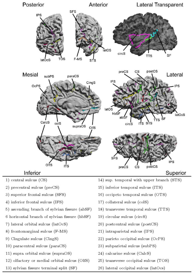
The complete set of candidate sulcal curves from which we select an optimal subset for constrained cortical registration
The surface based registration method we used here performs simultaneous parameterization and registration of the manually traced sulcal landmarks. The parameter space is the unit square which can be viewed as a flat mapping of each cortical hemisphere. In order to generate such a flat map with prealigned sulcal curves, we model the cortical surface as an elastic sheet and solve the associated linear elastic equilibrium equation subject to a sulcal matching constraint using the finite element method. Let φ = [φ1, φ2] be the two coordinates assigned to every point on a given cortical surface such that the coordinates φ satisfy the linear elastic equilibrium equation with Dirichlet boundary conditions on the boundary of each cortical hemisphere, represented by the corpus callosum. We match the most anterior and posterior points of the corpus callosum by constraining them to lie on two diagonally opposite corners of the unit square. The elastic strain energy E(φ) is given by:
| (1) |
where Dφ is the covariant derivative of the coordinate vector field φ. The integration is computed over the entire cortical surface, H, of each brain hemisphere. Let φB1 and φB2 denote the 2D coordinates to be assigned to hemispherical surfaces of two brains, B1 and B2. We then define the Lagrangian cost function C(φB1, φB2) as
| (2) |
where φB1(xk) and φB2(yk) denote the coordinates assigned to the sulcal landmarks xk ∈ B1, yk ∈ B2 and σ2 is a Lagrange multiplier. The landmarks correspond to uniformly sampled points along each sulcal curve. We refer the reader to (Joshi et al., 2007b,a) for implementation details.
When σ = 0 the constraints in Eq. 1 are ignored and we obtain a sulcally unconstrained registration. Note that even in this case, the closed curve through the corpus callosum, which bisects the brain into two hemispheres, is still mapped to the boundary of the unit square. As a result of this, and the mapping of the maximally anterior and posterior points on the callosal curve to opposite corners of the unit square, the sulcally unconstrained flat mappings still produce a degree of similarity in their mappings of the 26 sulcal curves.
We use these sulcally unconstrained mappings (σ = 0) to predict the errors that would result when constraining a subset of sulci to map to the same locations in the flat space. To do this we adopt a Gaussian model for errors in the registration of corresponding sulci and use conditional densities to model the effect of constraining a subset of these sulci. This model is described in Sec. 2.2. To test the accuracy of our predictions, we perform registrations with σ = 3 with the set C in Eq. 2 representing the subset of the 26 sulcal curves that are chosen for registration to constrain the mapping. The value for σ is chosen by studying the tradeoff between sulcal matching accuracy and overlaps/singularities in the flat map as explained in Joshi et al. (2007a). In that study, we found that lower values of sigma result in less accurate sulcal alignment and higher values cause singularities in the flat maps. σ = 3 was found to achieve optimal tradeoff between the sulcal matching accuracy and overlap in the flat maps. This method, for both σ = 0 and σ = 3, results in a bijective map of each brain hemisphere to the unit square such that the constrained sulci match in the flat space (Fig. 2). The point correspondence from one cortical surface hemisphere to the other is then obtained using the coordinate system of the common mapping to the unit square.
Fig. 2.
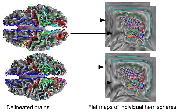
Registration of two cortical surfaces using sulcal matching constraint based on the flat mapping method
2.2 Registration Error
The point correspondence defined by registration allows us to map a point set from one brain to another brain. For every pair of registered hemispheres, we map the traced curves of of one brain, which we refer to as the subject, to the other, which we refer as the target. Note that the cost function in Eq. 2 is symmetric with respect to the two brains so that the designation of subject and target here are arbitrary. The registration is either sulcally unconstrained for error prediction, or constrained for validation. We parameterize each sulcal curve over [0, 1] and then compute S equidistant points on each sulcus.
The point to point errors en(s) are treated as S different samples of the error en, as illustrated in Fig. 4, where en(s) is the registration error in 3D coordinates for location s on the nth curve. Although the mapping function in Eq. 2 is symmetric with respect to the subject and target hemispheres that are coregistered, the mapping of sulci from subject to target will produce different errors than their mapping from target to subject. For symmetry, we repeat the procedure by interchanging subject and target brains.
Fig. 4.
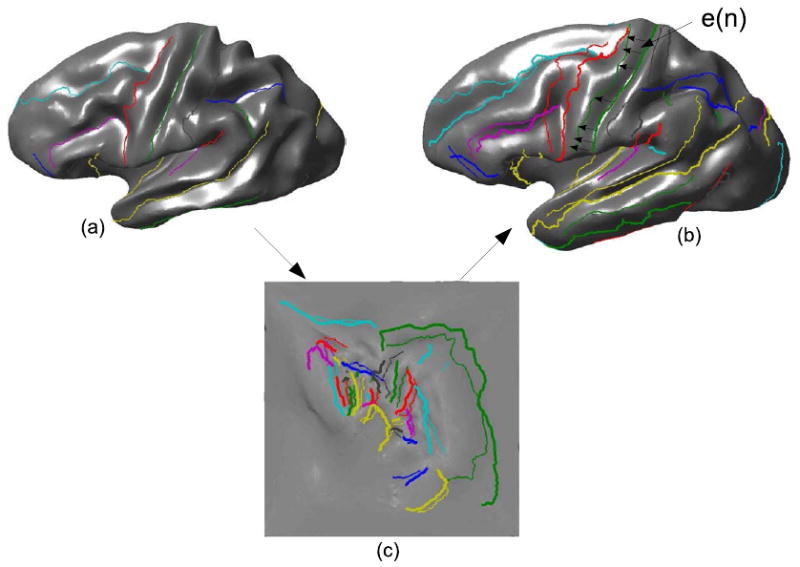
Unconstrained mapping of the sulcal curves of the subject brain to the target brain using square flat map as an intermediate common space: (a) subject brain with sulci, (b) target brain with its sulci and mapped sulci from the subject and (c) sulci mapped to square map.
The alignment error in a sulcus causes a registration error in the surrounding cortical area. Therefore, isolated sulcal curves (sulci that are great distance from other sulci) may have more impact on registration, since their misregistration will affect large cortical regions. To account for this effect, we parcellate the cortex into N = 26 regions by assigning each cortical point to the geodesically closest sulcal curve (Fig 3). The parcellation was performed for all M brain hemispheres. We then defined a weight function for the nth sulcus to be , where is the surface area of the nth parcellated region in the ith brain, and Ai is the total surface area of the ith hemisphere. Weights for each curve are then determined by averaging their respective areas over all subjects.
Fig. 3.
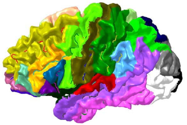
Parcellation of the cortex based on nearest sulcal curve
The final surface registration error metric is then defined as
| (3) |
where
and
represent the x, y, and z components of en, and  is the expectation operator. Below, we rewrite the error ER in (3) using the substitution:
| (4) |
in order to simplify subsequent analysis.
2.3 Probabilistic Model of the Sulcal Errors
We model the sulcal errors as jointly Gaussian random variables. We note that that the sulcal errors are zero mean. This is because subject and targets are chosen arbitrarily and they are also interchanged in the population. The distributions of sulcal errors are assumed to be symmetric around zero since in one sample we have a subject and a target, and in another they are interchanged to produce approximately the opposite displacements.
We describe computations for the x component of the error; similar computations are performed for y and z. The distribution model of is assumed to be Gaussian:
| (5) |
where Σx denotes the covariance matrix of Ex. Let denote the sample error for the kth pair of registered hemispheres, and P denote the number of such pairs. We compute the covariance from the set of errors as:
| (6) |
Therefore, the x component of the surface registration error in Eq. 3 can be expressed as:
| (7) |
Similarly, the total registration error is
We now want to predict the registration error when some of the sulci are explicitly constrained to register. We partition the curves into two sets: sulci F which are free (unconstrained) and sulci C which are constrained, so that {1…N} = F ∪ C. The primary assumption in the approach we describe in this paper is that the registration algorithm is well behaved in the sense that it does not create unnatural deformations on the unconstrained sulci when a subset of them are constrained. In other words, if we constrain some sulci to register, the distribution of the remaining ones would be the same as if the constrained ones matched simply by chance. Under this assumption we can compute registration errors for the unconstrained sulci using a conditional density, with the condition on the constrained sulci having zero error. In other words we model the registration errors for the unconstrained sulci using a conditional form of the distribution of the original jointly Gaussian density. The probability density of a jointly Gaussian vector, conditioned on some of its elements being zero, is also jointly Gaussian. Therefore, the registration error after matching the sulci from set C can be obtained using the conditional expectation:
| (8) |
where is the conditional covariance matrix of the error terms corresponding to free sulci. By rearranging sulci so that free sulci precede the constrained ones, we can partition the covariance matrix as:
| (9) |
where and are the error covariances for free sulci and constrained sulci respectively, and and are the cross-covariances.
The conditional covariance is given by:
| (10) |
which is the Schur complement of in Σx (Mardia et al., 1979). The estimated registration error after constraining a subset of sulci is then:
| (11) |
This formula allows us to estimate the x component of the registration error for a particular combination of constrained sulci and free sulci. The total constrained registration error is evaluated by adding the x, y, and z components.
| (12) |
We can use this formula to estimate the total registration errors for all combinations of sulcal subsets, where Nc is the number of constrained sulci, and choose the subset that minimizes this error.
We model each of the x, y, and z components of the sulcal errors independently. Ideally, the correlation among the x, y and z components of the errors in the sulcal locations should be taken into consideration. We make the simplifying assumption that this correlation is zero resulting in a factor 3 reduction in the size of the covariance matrices that need to be inverted in the estimation step (Eq. 10). This makes our model more stable because we have to estimate fewer parameters, which we compute from a relatively small population of 12 brains. When we began this work, we tested both approaches, and found that the assumption of independence between x, y, and z components produced more consistent and stable results.
The registration error is defined as a weighted sum of sulcal errors (Eq. 3). Whenever a sulcus is missing, we assign zero sulcal error since meaningful point correspondence does not exist in that case. Also, when a sulcus is constrained to align, we assign zero sulcal error. Therefore the sum in Eq. 3 is effectively computed over the entire set of sulci. Consequentially, the registration error effectively quantifies alignment of the entire cortex, and does not depend on the number of measurements and constrained/free sulci.
3 Results
The sulci of 24 brains (48 hemispheres), were traced. Our tracings, consisting of 26 candidate sulci per hemisphere (Fig. 1), were verified and corrected whenever necessary by a neuroanatomist. We divided the brains into two subsets, a training set of 12 brains (24 hemispheres) and a testing set of 12 brains (24 hemispheres), in order to check:
Accuracy of the estimator: whether the errors predicted by our method are close to the actual errors after registration.
Generalizability of the results to other datasets: if we chose a different dataset (testing set) of brains and sulci, whether the registration errors remain similar to those for the training dataset.
We applied our algorithm on the 12 training brains as described in Sec. 3.1, to find the optimal subsets of sulci that minimize the registration error. To test if the predicted errors generalize to other datasets, in Sec. 3.2 we used the 12 testing brains to calculate the actual registration errors for all optimal subsets identified in the training brains.
3.1 Optimal sulcal set prediction
We performed sulcally unconstrained mappings for all the 12 brains from the training set by directly minimizing Eq. 1 for each hemisphere separately, instead of doing pairwise registrations using Eq. 2 with σ = 0, since the optimization in Eq. 2 becomes separable in the sulcally unconstrained case σ = 0. Using the flat maps of the 24 hemispheres we computed samples of sulcal errors , and , with S = 10 equidistant points for each sulcus, for all possible pairwise combinations of hemispheres as described in Sec. 2.2. The resulting sample covariance matrices for these errors are shown in Fig. 5. Non-zero off-diagonal elements indicate that the errors are correlated among sulci, and thus constraining them ill affect the registration error for the others. The correlation structure of the sulcal errors depends on the sulcal locations in the flat maps. Here we use square maps as discussed in Sec. 2.2, but we expect that our results should be robust with respect to the mapping method.
Fig. 5.

Sample covariance matrices for the x, y, and z components (in mm2) of the registration error, represented as color coded images.
By applying Eq. 12 to all subsets of a given number of constrained curves, we identified the subset that minimizes the registration error. The optimal subsets of curves is given in Fig. 6 for all numbers of constrained sulci from 1 to 26. The estimates of the registration error obtained according to Eq. 12 are listed in the column of Fig. 6 titled ‘Est Error’. We also calculated the sulcal registration errors for each of these optimal subsets by doing actual registration (Fig. 6, last two columns for the training and testing set of brains). In order to perform actual registration, we chose σ = 3 as discussed in (Joshi et al., 2007a) for the constrained subset of sulci. Comparing estimated and actual registration errors, in Fig. 6, we see that the predicted values are close to those obtained when actually constraining the optimal subsets of curves.
Fig. 6.

Optimal subsets of sulci for cortical registration. Each row gives the indices of the optimal subset of sulci that minimize the registration error against all other combinations with an equal number of constrained curves (also see Fig. 1). The three right columns show respectively: Estimated (est) error for the optimal subset of curves computed from the conditional error covariance matrices for the training data as defined in Eq. 12; actual registration error (tm) computed from the coregistered brains from the training data for this set of constraint curves; and actual registration error (tst) computed from coregistered brains from the test data.
Fig. 8 shows an example of the empirical distribution of the x-component of the registration error (Eq. 4) for the superior frontal sulcus. The Q-Q plot (Fig. 8b) indicates small deviation from normality. A Lilliefors test rejected the null hypothesis of normality for the errors , and for many sulci, and therefore our Gaussianity assumption is not fully satisfied. This is not surprising, since for example errors are naturally bounded by the size of the brains and therefore some deviation from normality was anticipated. However, the distributions were unimodal and the predicted errors of our model are in accordance with the actual ones (Fig. 6), indicating that our distributional assumptions are reasonable.
Fig. 8.
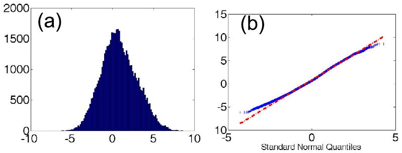
(a) Empirical distribution of the x-component of the registration error in the superior frontal sulcus; (b) Q-Q plot of the error against a normal distribution.
3.2 Generalizability
In order to check the generalizability of the results, we used the 12 brains from the testing set. We performed pairwise registrations of the testing brains constraining the optimal subsets of sulci to be the same as the ones identified from the training set (for all subsets from 1 to 26 sulci). These optimal sets are given in Fig. 6, and the testing set errors are given in the last column of Fig. 6, and also in Fig. 9. The average registration errors in this case were again close to the predicted errors as shown in Fig. 6 and Fig. 9. To further test our method, we subjectively selected a set of 6 curves to be constrained, namely CS, SFS, STS, IPS, CingS and CalcS. This selection was based primarily on the length of sulci and second on a reasonable spread throughout the cortex. The algorithm predicted an error of 194.36mm2 and the actual error was 200.03mm2. The optimal set (SFS, STS, OTS, postCS, IPS, and CalcS) found by our method had predicted an error of 167.19mm2 and the actual error was 164.77mm2, which is better than our subjectively selected subset. We anticipate that in general the curves selected by our method should be superior to those selected on an intuitive basis, since various confounding effects due to elastic flat mapping, correlations in errors as well as population variability are accounted for in the algorithm.
Fig. 9.

Plot of registration errors: Estimated (est) error for the optimal subset of curves computed from the conditional error covariance matrices for the training data; actual registration error (tm) computed from the coregistered brains from the training data for this set of constraint curves; and actual registration error (tst) computed from coregistered brains from the test data.
4 Discussion and Conclusion
We have described a general procedure for selecting subsets of sulcal landmarks for use in constrained cortical registration. The procedure can be used to reduce the time required for manual labeling of sulci in group studies of cortical anatomy and function.
The optimal subsets of curves, shown in Fig. 6, provide an idea of the criteria used by the method to select curves. First notice that the central sulcus is not selected for protocols with a small number of curves (less than 16). This is probably because sulci that are most stable and consistent among brains, such as the central sulcus, may tend to align well even without explicitly tracing them. Therefore, they may not improve the registration error sufficiently to justify their inclusion in the tracing protocol. Furthermore, short sulci neighboring other candidate curves are not preferred by the algorithm, because they do not sufficiently add constraints to the registration. For example, the paracentral sulcus which is close to the cingulate sulcus, and the subparietal sulcus which is close to the cingulate and the parieto-occipital sulcus are not preferred by the method.
On the other hand, one of the most important sulci for surface based registration seems to be the superior temporal sulcus with its upper branch. This is possibly for two reasons: (1) it is one of the longest sulci and hence aligning it will help register a large region of the brain; (2) in cortical flat maps where the corpus callosum is mapped on the edges of a unit square, such as in our method in Fig. 2, the temporal lobe is far from the edge of the unit square, which always maps to the corpus callosum by construction. Therefore when no sulcal constraint are placed in the temporal lobe, we tend to see large registration error. Consequentially, it is important to align at least one sulcus in temporal lobe accurately, and hence it is selected by our method. The other important sulcus is the Calcarine, which is not as long as the superior temporal sulcus, but is highly variable among subjects.
Our mapping method biases sulcal selection to the extent that corpus callosum is already aligned when performing the flattening. Since we align the corpus callosum for the mapping, the registration errors tend to be smaller in this region, which biases our optimal curve set. This is not necessarily a disadvantage. Every surface registration method requires some initial mapping. For example, surface registration in FreeSurfer and BrainVoyager is properly initialized by 1) volumetric alignment of brain scans to the Talairach space, and then 2) inflation of surfaces to the unit sphere. Our goal is to define optimal sets of curves for registration; in this paper we provide the optimal sets of curves when the registration method in (Joshi et al., 2007b) is used. If another registration method is chosen, it is straightforward to extend our method to find corresponding optimal sets of curves.
Registration error always remains when only a subset of sulci is used for registration. Whether this is acceptable or not depends on the particular study being contemplated. For example, anatomical studies (Thompson et al., 2001b; Sowell et al., 2002; Changeux, 1998; Gogtay et al., 2004) require high accuracy and might need more sulci, whereas some functional studies, such as those using low resolution magnetoencephalography data (Pantazis et al., 2005), can tolerate higher registration error. Fig. 6 can be used as a guideline: based on the registration accuracy required, a different number of curves may be used.
Our method determines the subset of sulci to be delineated in a registration study based solely on the registration error. However, some changes in the selected subset can be made based on other practical considerations, such as convenience in tracing. For instance, identification and tracing of the central sulcus is always easy and it could be helpful in identifying the surrounding sulci. Therefore we expect that it would be typically included in a tracing protocol. Furthermore, for neuroscience studies focusing on particular cortical regions, the registration error metric defined in Sec. 2.2 can be modified by assigning more weight to the regions of interest. For example, in language studies interested in activation in the temporal lobe and Broca's area we can increase the weights wn in Eq. 3 for STS, ITS, SF, abSF, hbSF, IFS. Our method would then favor the aforementioned sulci and produce different sets of optimal curves than the ones displayed in Fig. 6.
In this paper, we have used a registration method which constrains the endpoints of the sulci to match. While allowing sulcal curves to slide as opposed to uniformly sampling them can lead to slightly better results (Leow et al., 2005), uniform sampling with matching endpoints has been used in a number of publications and has led to useful and important results. e.g. (Gogtay et al., 2004; Thompson and Toga, 1996; Thompson et al., 2003; Sowell et al., 2003; Thompson et al., 2001a, 1997). This approximation makes the analysis tractable as opposed to letting the sulcal curves slide. The error in the sulcal curves was normalized and weighted by the area surrounding each curve. Consequently the error does not depend on the length of the curve but rather the area surrounding the curve.
Errors and variability in identifying cortical landmarks are a common problem concerning all landmark based techniques and can affect the registration error. However, they are beyond the scope of this paper. For this particular study the curves were identified and cross-checked by an expert neuroanatomist. Inter- and intra-rater variability is typically minimized by appropriate training and cross checking of traces. A possible extension of our method could allow modeling of intra/inter-rater variability in identifying sulci, so that sulci with high rater variability are penalized in the protocol selection process.
Even though we used 2D flat maps, other registration approaches are also possible with our method, such as spherical registrations used in FreeSurfer and BrainVoyager. Our methodology readily extents to other landmark based registration methods in which the goal is to select an optimal subset of landmarks for large scale studies, from a set of candidate landmarks. Finally, it can possibly be applied to other problems of computer vision such as robotics (Madsen and Andersen, 1998; Wang and Song, 2009; Greiner and Isukapalli, 1994), terrain matching (Olson, 2000), face recognition (Beumer et al., 2006), etc. for aiding optimal landmark selection.
Fig. 7.
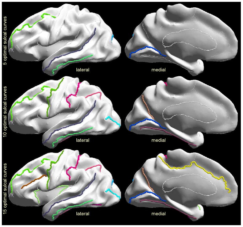
Optimal sulcal sets for 5, 10, and 15 curves.
Fig. 10.
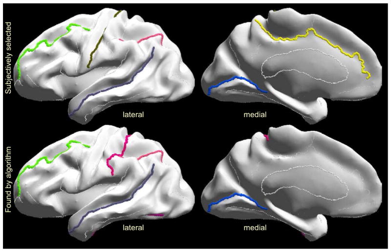
Top row: subjective selection of 6 curves, with preference on long sulci distant from each other that are expected to minimize cortical registration error; bottom row: optimal sulcal set with the 6 curves selected by our method.
Acknowledgments
This work is supported under grants R01 EB002010, P41 RR013642 and NIH/NIDCD (DC008308/DC008583).
Footnotes
Publisher's Disclaimer: This is a PDF file of an unedited manuscript that has been accepted for publication. As a service to our customers we are providing this early version of the manuscript. The manuscript will undergo copyediting, typesetting, and review of the resulting proof before it is published in its final citable form. Please note that during the production process errors may be discovered which could affect the content, and all legal disclaimers that apply to the journal pertain.
References
- Besl P, McKay H. A method for registration of 3-D shapes. IEEE Transactions on pattern analysis and machine intelligence. 1992;14(2):239–256. [Google Scholar]
- Beumer GM, Tao Q, Bazen AM, Veldhuis RNJ. FGR '06: Proceedings of the 7th International Conference on Automatic Face and Gesture Recognition. IEEE Computer Society; Washington, DC, USA: 2006. A landmark paper in face recognition; pp. 73–78. [Google Scholar]
- Blanton RE, Levitt JG, Thompson PM, Narr KL, Capetillo-Cunliffe L, Nobel A, McCracken JDSJT, Toga AW. Mapping cortical asymmetry and complexity patterns in normal children. Psychiatry Res. 2001 Jul;107:29–43. doi: 10.1016/s0925-4927(01)00091-9. [DOI] [PubMed] [Google Scholar]
- Caunce A, Taylor CJ. 3d point distribution models of the cortical sulci. ICCV. 1998:402–407. [Google Scholar]
- Changeux J. Drug use and abuse. Daedalus. 1998:145–165. [Google Scholar]
- Chui H, Rangarajan A. A new point matching algorithm for non-rigid registration. Computer Vision and Image Understanding. 2003;89(23):114–141. [Google Scholar]
- Cootes T, Taylor C. Anatomical statistical models and their role in feature extraction. British Journal of Radiology. 2004;77(Special Issue 2):S133. doi: 10.1259/bjr/20343922. [DOI] [PubMed] [Google Scholar]
- Fischl B, Sereno MI, Tootell RBH, Dale AM. High-resolution inter-subject averaging and a coordinate system for the cortical surface. Human Brain Mapping. 1998;8:272–284. doi: 10.1002/(SICI)1097-0193(1999)8:4<272::AID-HBM10>3.0.CO;2-4. [DOI] [PMC free article] [PubMed] [Google Scholar]
- Goebel R, Esposito F, Formisano E. Analysis of functional image analysis contest (FIAC) data with brainvoyager QX: From single-subject to cortically aligned group general linear model analysis and self-organizing group independent component analysis. Human Brain Mapping. 2006;27(5):392. doi: 10.1002/hbm.20249. [DOI] [PMC free article] [PubMed] [Google Scholar]
- Goghari V, Rehm K, Carter C, Macdonald A. Sulcal thickness as a vulnerability indicator for schizophrenia. The British Journal of Psychiatry. 2007;191(3):229. doi: 10.1192/bjp.bp.106.034595. [DOI] [PubMed] [Google Scholar]
- Gogtay N, Giedd J, Lusk L, Hayashi K, Greenstein D, Vaituzis A, Nugent T, Herman D, Clasen L, Toga A, et al. Dynamic mapping of human cortical development during childhood through early adulthood. Proceedings of the National Academy of Sciences. 2004;101(21):8174. doi: 10.1073/pnas.0402680101. [DOI] [PMC free article] [PubMed] [Google Scholar]
- Greiner R, Isukapalli R. Learning to select useful landmarks. National Conference on Artificial Intelligence. 1994:1251–1256. [Google Scholar]
- Hoffman H, Richards T, Coda B, Bills A, Blough D, Richards A, Sharar S. Modulation of thermal pain-related brain activity with virtual reality: evidence from fMRI. NeuroReport. 2004;15(8):1245. doi: 10.1097/01.wnr.0000127826.73576.91. [DOI] [PubMed] [Google Scholar]
- Joshi A, Shattuck D, Thompson P, Leahy R. A finite element method for elastic parameterization and alignment of cortical surfaces using sulcal constraints. 4th IEEE International Symposium on Biomedical Imaging: From Nano to Macro, 2007. ISBI 2007. 2007a:640–643. [Google Scholar]
- Joshi AA, Shattuck DW, Thompson PM, Leahy RM. Surface-constrained volumetric brain registration using harmonic mappings. IEEE Trans Med Imaging. 2007b;26(12):1657–1669. doi: 10.1109/tmi.2007.901432. [DOI] [PMC free article] [PubMed] [Google Scholar]
- Kippenhan J, Olsen R, Mervis C, Morris C, Kohn P, Meyer-Lindenberg A, Berman K. Genetic Contributions to Human Gyrification: Sulcal Morphometry in Williams Syndrome. Journal of Neuroscience. 2005;25(34):7840–7846. doi: 10.1523/JNEUROSCI.1722-05.2005. [DOI] [PMC free article] [PubMed] [Google Scholar]
- Leow A, Yu C, Lee S, Huang S, Protas H, Nicolson R, Hayashi K, Toga A, Thompson P. Brain structural mapping using a novel hybrid implicit/explicit framework based on the level-set method. NeuroImage. 2005;24(3):910–927. doi: 10.1016/j.neuroimage.2004.09.022. [DOI] [PubMed] [Google Scholar]
- Luders E, Rex DE, Narr KL, Woods RP, Jancke L, Thompson PM, Mazziotta JC, Toga AW. Relationships between sulcal asymmetries and corpus callosum size: gender and handedness effects. Cereb Cortex. 2003 Oct;13(10):1084–1093. doi: 10.1093/cercor/13.10.1084. [DOI] [PubMed] [Google Scholar]
- Madsen C, Andersen C. Optimal landmark selection for triangulation of robot position. Robotics and Autonomous Systems. 1998;23(4):277–292. [Google Scholar]
- Mardia K, Kent J, Bibby J. Multivariate Analysis. Academic Press; 1979. [Google Scholar]
- Nahas GG, Burks TF, editors. Drug Abuse in the Decade of the Brain. IOS Press; 1997. [Google Scholar]
- Narr K, Thompson P, Sharma T, Moussai J, Zoumalan C, Rayman J, Toga A. Three-dimensional mapping of gyral shape and cortical surface asymmetries in schizophrenia: gender effects. Am J Psychiatry. 2001 Feb;158(2):244255. doi: 10.1176/appi.ajp.158.2.244. [DOI] [PMC free article] [PubMed] [Google Scholar]
- O'Donnell S, Noseworthy M, Levine B, Dennis M. Cortical thickness of the frontopolar area in typically developing children and adolescents. Neuroimage. 2005a;24(4):948–954. doi: 10.1016/j.neuroimage.2004.10.014. [DOI] [PubMed] [Google Scholar]
- O'Donnell S, Noseworthy M, Levine B, Dennis M. Cortical thickness of the frontopolar area in typically developing children and adolescents. Neuroimage. 2005b;24(4):948–954. doi: 10.1016/j.neuroimage.2004.10.014. [DOI] [PubMed] [Google Scholar]
- Olson C. Landmark selection for terrain matching. Proceedings of the IEEE International Conference on Robotics and Automation. 2000:1447–1452. [Google Scholar]
- Pantazis D, Joshi AA, Jintao J, Shattuck DW, Bernstein LE, Damasio H, Leahy RM. Comparison of landmark-based and automatic methods for cortical surface registration. NeuroImage. 2009 doi: 10.1016/j.neuroimage.2009.09.027. in press. [DOI] [PMC free article] [PubMed] [Google Scholar]
- Pantazis D, Nichols TE, Baillet S, Leahy R. A comparison of random field theory and permutation methods for the statistical analysis of meg data. Neuroimage. 2005 Apr;25(2):383–394. doi: 10.1016/j.neuroimage.2004.09.040. [DOI] [PubMed] [Google Scholar]
- Rangarajan A, Chui H, Mjolsness E, Pappu S, Davachi L, Goldman-Rakic P, Duncan J. A robust point-matching algorithm for autoradiograph alignment. Medical Image Analysis. 1997;1(4):379–398. doi: 10.1016/s1361-8415(97)85008-6. [DOI] [PubMed] [Google Scholar]
- Shattuck DW, Joshi AA, Pantazis D, Kan E, Dutton RA, Sowell ER, Thompson PM, Toga AW, Leahy RM. Semi-automated method for delineation of landmarks on models of the cerebral cortex. Journal of Neuroscience Methods. 2009;178(2):385–392. doi: 10.1016/j.jneumeth.2008.12.025. [DOI] [PMC free article] [PubMed] [Google Scholar]
- Shattuck DW, Leahy RM. Brainsuite: An automated cortical surface identification tool. Medical Image Analysis. 2002;8(2):129–142. doi: 10.1016/s1361-8415(02)00054-3. [DOI] [PubMed] [Google Scholar]
- Sowell ER, Peterson BS, Thompson PM, Welcome1 SE, Henkenius1 AL, Toga AW. Mapping cortical change across the human life span. Nature Neuroscience. 2003;6:309–315. doi: 10.1038/nn1008. [DOI] [PubMed] [Google Scholar]
- Sowell ER, Thompson PM, Rex D, Kornsand D, Tessner KD, Jernigan TL, Toga AW. Mapping sulcal pattern asymmetry and local cortical surface gray matter distribution in vivo: maturation in perisylvian cortices. Cereb Cortex. 2002 Jan;12(1):17–26. doi: 10.1093/cercor/12.1.17. [DOI] [PubMed] [Google Scholar]
- Sozou PD, Cootes TF, Taylor CJ, Mauro ECD, Lanitis A. Non-linear point distribution modelling using a multi-layer perceptron. Image Vision Comput. 1997;15:457–463. [Google Scholar]
- Thompson P, Hayashi K, De Zubicaray G, Janke A, Rose S, Semple J, Doddrell D, Cannon T, Toga A. Detecting dynamic and genetic effects on brain structure using high-dimensional cortical pattern matching. IEEE International Symposium on Biomedical Imaging. 2002;2002:473. doi: 10.1109/ISBI.2002.1029297. [DOI] [PMC free article] [PubMed] [Google Scholar]
- Thompson P, Hayashi K, de Zubicaray G, Janke A, Rose S, Semple J, Herman D, Hong M, Dittmer S, Doddrell D, et al. Dynamics of gray matter loss in Alzheimer's disease. Journal of Neuroscience. 2003;23(3):994–1005. doi: 10.1523/JNEUROSCI.23-03-00994.2003. [DOI] [PMC free article] [PubMed] [Google Scholar]
- Thompson P, Vidal C, Giedd J, Gochman P, Blumenthal J, Nicolson R, Toga A, Rapoport J. Mapping adolescent brain change reveals dynamic wave of accelerated gray matter loss in very early-onset schizophrenia. Proceedings of the National Academy of Sciences of the United States of America. 2001a;98(20):11650. doi: 10.1073/pnas.201243998. [DOI] [PMC free article] [PubMed] [Google Scholar]
- Thompson PM, MacDonald D, Mega MS, Holmes CJ, Evans AC, Toga AW. Detection and mapping of abnormal brain structure with a probabilistic atlas of cortical surfaces. Journal of Computer Assisted Tomography. 1997 Jul.-Aug;21(4):567–581. doi: 10.1097/00004728-199707000-00008. [DOI] [PubMed] [Google Scholar]
- Thompson PM, Mega MS, Toga AW. Disease-specific probabilistic brain atlases. Procedings of IEEE International Conference on Computer Vision and Pattern Recognition. 2000:227–234. doi: 10.1109/MMBIA.2000.852382. [DOI] [PMC free article] [PubMed] [Google Scholar]
- Thompson PM, Mega MS, Vidal C, Rapoport J, Toga AW. Detecting disease-specific patterns of brain structure using cortical pattern matching and a population-based probabilistic brain atlas. IPMI2001. LNCS. 2001b:488–501. doi: 10.1007/3-540-45729-1_52. [DOI] [PMC free article] [PubMed] [Google Scholar]
- Thompson PM, Toga AW. A surface-based technique for warping 3-dimensional brain. IEEE Transactions on Medical Imaging. 1996;15(4):1–16. doi: 10.1109/42.511745. [DOI] [PubMed] [Google Scholar]
- Tosun D, Rettmann ME, Prince JL. Mapping techniques for aligning sulci across multiple brains. Medical Image Analysis. 2005;8(3):295–309. doi: 10.1016/j.media.2004.06.020. [DOI] [PMC free article] [PubMed] [Google Scholar]
- Van Essen D. A population-average, landmark-and surface-based (PALS) atlas of human cerebral cortex. Neuroimage. 2005;28(3):635–662. doi: 10.1016/j.neuroimage.2005.06.058. [DOI] [PubMed] [Google Scholar]
- Wang M, Song Z. Improving target registration accuracy in image-guided neurosurgery by optimizing the distribution of fiducial points. The International Journal of Medical Robotics and Computer Assisted Surgery. 2009;5(1):1478–5951. doi: 10.1002/rcs.227. [DOI] [PubMed] [Google Scholar]
- Wang Y, Chiang MC, Thompson PM. Automated surface matching using mutual information applied to Riemann surface structures. MICCAI 2005, LNCS. 2005;3750:666–674. doi: 10.1007/11566489_82. [DOI] [PubMed] [Google Scholar]