3D image segmentation of deformable objects with joint shape-intensity prior models using level sets

Abstract

We propose a novel method for 3D image segmentation, where a Bayesian formulation, based on joint prior knowledge of the object shape and the image gray levels, along with information derived from the input image, is employed. Our method is motivated by the observation that the shape of an object and the gray level variation in an image have consistent relations that provide configurations and context that aid in segmentation. We define a maximum a posteriori (MAP) estimation model using the joint prior information of the object shape and the image gray levels to realize image segmentation. We introduce a representation for the joint density function of the object and the image gray level values, and define a joint probability distribution over the variations of the object shape and the gray levels contained in a set of training images. By estimating the MAP shape of the object, we formulate the shape-intensity model in terms of level set functions as opposed to landmark points of the object shape. In addition, we evaluate the performance of the level set representation of the object shape by comparing it with the point distribution model (PDM). We found the algorithm to be robust to noise and able to handle multidimensional data, while able to avoid the need for explicit point correspondences during the training phase. Results and validation from various experiments on 2D and 3D medical images are shown.

1. Introduction

The accurate segmentation and quantitative analysis of structures in an image is a fundamental issue in a variety of applications including medical image processing, computer vision and pattern recognition.

In the active contour approach (snakes) of Kass et al. (1987), energy minimizing parametric contours with smoothness constraints are deformed according to the image data. Unlike level set implementations (Osher and Sethian, 1988), the direct implementation of this energy model is not capable of handling topological changes of the evolving contour without explicit discrete pixel manipulations. Usually, they can detect only objects with edges defined by the gradient.

Curve evolution methods based on level set (Osher and Sethian, 1988) have been used extensively for segmentation, because they allow for automatic changes in the topology. Novel geometric models of active contours have been proposed based on curve evolution and geometric flows (Caselles et al., 1993, 1997; Malladi et al., 1993). By using the level-sets-based numerical algorithm, several objects can be segmented simultaneously (Yang et al., 2003, 2004; Tsai et al., 2003b).

Recently, Chan and Vese (2001) have proposed an active contour model using a Mumford–Shah functional, based on techniques of curve evolution and level sets for segmentation. In the level set formulation of the Mumford–Shah functional, the problem becomes a “mean-curvature flow”. This model can detect objects whose boundaries are not necessarily fully defined by gradient data, for instance objects with very smooth boundaries or even with discontinuous boundaries can be inferred. In addition, since the model has a level set formulation, changes of topology are allowed, interior contours can be automatic detected, and the initial curve can be placed anywhere in the image.

Image gray level based methods often face difficult challenges such as poor image contrast, noise, and missing or diffuse boundaries. Prior model based algorithms can often solve this problem. Chen et al. (2002) use an “average shape” as the shape prior term in their geometric active contour model. Cootes et al. (1994) find corresponding points across a set of training images and construct a statistical model of shape variation from the point positions. Wang and Staib (1998) propose a systematic approach to determine an object's boundary as well as the correspondence of boundary points to a model by constructing a statistical model of shape variation. Staib and Duncan (1992) incorporate global shape information into the segmentation process by using an elliptic Fourier decomposition of the boundary and placing a Gaussian prior on the Fourier coefficients. Zeng et al. (1999) develop a coupled surfaces algorithm to segment the cortex by using a thickness prior constraint. Leventon et al. (2000) extend Caselles et al.'s (1997) geodesic active contours by incorporating shape information into the evolution process. They use principal component analysis (PCA) (Cootes et al., 1994) and level set functions of the object boundaries to form a statistical shape model from a training set. The segmenting curves evolve according to the image gradient and a maximum a posteriori (MAP) estimates of shape and pose. More recently, Tsai et al. (2001, 2003a) use the same implicit representation of the object boundary presented in Leventon et al. (2000) and manipulate the parameters of this implicit model to minimize the region-based energy functional proposed by Chan and Vese (2001) and Yezzi et al. (1999) to realize image segmentation. In our previous work, we adopt a level set approach using prior information of both the shape of an object and its neighbors (Yang et al., 2003, 2004). Tsai et al. describe a similar approach (Tsai et al., 2003b), which uses a global multi-shape model. We feel that our approach is more flexible in the modeling of joint priors and accommodates situations with limited inter-object information and variation in contrast and discernability among the objects.

In addition to the shape prior based segmentation methods, Cootes et al. use statistical models of both shape and texture as deformable anatomical atlases (Cootes et al., 1999, 2001). The modeled structure can be located by finding the parameters, which minimize the difference between the synthesized model image and the target image in conjunction with the statistical model of the shape based on landmark points and texture. The point correspondence problem needs to be taken care of and is difficult in 3D images, although minimum description length (MDL) (Davies et al., 2002) approaches can be used to define point correspondences. Further evaluation of different 3D correspondence methods are presented by Styner et al. (2003).

Our work shares the observation that an object to be detected and the gray level variation in an image could have a consistent relation that can aid in the delineation. Our model is based on a MAP framework using the shape-intensity joint prior information. We introduce a new representation for the shape-intensity joint density function and define the corresponding probability distribution. We evaluate this level set distribution model by comparing it with the traditional point distribution model (Cootes et al., 1994) using the χ² test. Formulating the segmentation as a MAP estimation of the shape of the object and modeling in terms of level set function, we compute the associated Euler–Lagrange equation. We avoid the need for explicit point correspondences during the training phase by using a level set representation of the object shape. The contour evolves both according to the shape-intensity joint prior information and the image gray level information.

2. Description of the model

2.1. MAP framework with shape-intensity joint prior

The shape of an object is always dependent on the gray level variation in an image. Segmentation can be made easier if suitable models containing such relationship priors are available. A probabilistic formulation is a powerful approach to deformable models. Deformable models can be fit to the image data by finding the model shape parameters that maximize the posterior probability. Consider an image I that has an object 𝒮 of interest; a MAP framework can be used to realize image segmentation combining prior information and image information

$$\begin{array}{cc}\hfill \widehat{𝒮},{\widehat{I}}_{𝒮}& =\arg \underset{𝒮,I_{𝒮}}{\max }p(𝒮,I_{𝒮}\mid I)\hfill \\ \hfill & =\arg \underset{𝒮,I_{𝒮}}{\max }p(I\mid 𝒮,I_{𝒮})p(𝒮,I_{𝒮}),\hfill \end{array}$$ (1)

where I_𝒮 is the synthetic model image of image I; Î_𝒮 is the estimation of the synthetic image I_𝒮 Since our main concern is the segmentation of the object 𝒮̂, we assume that the synthetic image I_𝒮 is very close to the real image I, thus I_𝒮 ≈ I, and Eq. (1) becomes

$$\widehat{𝒮}=\arg \underset{𝒮}{\max }p(𝒮,I_{𝒮}\mid I)\approx \arg \underset{𝒮}{\max }p(I\mid 𝒮,I_{𝒮}\approx I)p(𝒮,I)$$ (2)

p(I|𝒮, I_𝒮) is the image gray level information based term. In 3D, assuming gray level homogeneity within the object, we use the following imaging model (Chan and Vese, 2001):

$$\begin{array}{cc}\hfill p(I\mid 𝒮,I_{𝒮})=& {\Pi }_{(x,y,z)\text{inside}\left(𝒮\right)}\exp [-{(I(x,y,z)-c_1)}^2∕\left(2{\sigma }_1^2\right)]\hfill \\ \hfill & \times {\Pi }_{(x,y,z)\text{outside}\left(𝒮\right),\text{inside}\left({\Omega }_{𝒮}\right)}\hfill \\ \hfill & \exp [-{(I(x,y,z)-c_2)}^2∕\left(2{\sigma }_2^2\right)],\hfill \end{array}$$ (3)

where c₁ and σ₁ are the average and variance of I inside 𝒮, c₂ and σ₂ are the average and variance of I outside 𝒮 but also inside a certain domain Ω_𝒮 that contains 𝒮. p(𝒮, I) is the joint density function of shape 𝒮 and image intensity I. It contains the shape prior information, the intensity prior information, as well as their relation.

2.2. Shape-intensity joint prior model

Instead of using a point model to represent the object as was done in (Cootes et al., 1994, 1999), we choose level sets (Osher and Sethian, 1988) as the representation of the object to build a model for the shape-intensity joint prior, and then define the joint probability density function in Eq. (2).

Consider a training set of n aligned images {I₁, I₂, …, I_n}, with an object of interest in each image. The surfaces of the n objects in the training set are embedded as the zero level sets of n separate higher dimensional level set functions {ψ₁, ψ₂, …, ψ_n} with negative distances inside and positive distances outside the object. Using the technique developed in (Leventon et al., 2000), each of the I_i and ψ_i is placed as a column vector with N^d elements, where d is the number of spatial dimensions and N^d is the number of samples of each level set function or the number of pixels of each image. We can use vector ${[{\Psi }_i^{\mathrm{T}},I_i^{\mathrm{T}}]}^{\mathrm{T}}$ as the representation of the object and intensity values. Thus, the corresponding training set is $\{{[{\Psi }_1^{\mathrm{T}},I_1^{\mathrm{T}}]}^{\mathrm{T}},{[{\Psi }_2^{\mathrm{T}},I_2^{\mathrm{T}}]}^{\mathrm{T}},\dots ,{[{\Psi }_n^{\mathrm{T}},I_n^{\mathrm{T}}]}^{\mathrm{T}}\}$ Our goal is to build a shape-intensity model over the distribution of the level set function and intensity pair.

The mean and variance of the shape-intensity pair can be computed using PCA (Cootes et al., 1994). The mean shape-intensity pair, $\overline{{[{\Psi }^{\mathrm{T}},I^{\mathrm{T}}]}^{\mathrm{T}}}=(1∕n){\Sigma }_{i=1}^n{[{\Psi }_i^{\mathrm{T}},I_i^{\mathrm{T}}]}^{\mathrm{T}}$, is subtracted from each ${[{\Psi }_i^{\mathrm{T}},I_i^{\mathrm{T}}]}^{\mathrm{T}}$ to create the deviation from the mean. Each such deviation is placed as a column vector in a 2N^d × n dimensional matrix Q. Using singular value decomposition (SVD), Q = UΣV ^T, U is a 2N^d × n matrix whose column vectors represent the set of orthogonal modes of shape-intensity variation and Σ is a n × n diagonal matrix of corresponding singular values. An estimate of the shape-intensity pair [ψ^T, I^T]^T can be represented by k principal components and a k dimensional vector of coefficients (where k < n), α (Cootes et al., 1994)

$$\widetilde{\left[\begin{array}{c}\hfill \Psi \hfill \\ \hfill I\hfill \end{array}\right]}=\overline{\left[\begin{array}{c}\hfill \Psi \hfill \\ \hfill I\hfill \end{array}\right]}+U_k\alpha ,$$ (4)

where U_k is a 2N^d × k matrix consisting of the first k columns of matrix U.

Under the assumption of a Gaussian distribution of a shape-intensity pair represented by α, the joint probability of a certain shape 𝒮 and the related image intensity I, p(𝒮, I) can be represented by

$$p\left(\alpha \right)=\frac{1}{\sqrt{{\left(2\pi \right)}^k\left|{\Sigma }_k\right|}}\exp \left[-\frac{1}{2}{\alpha }^{\mathrm{T}}{\Sigma }_k^{-1}\alpha \right].$$ (5)

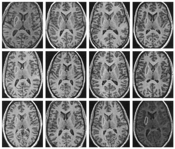
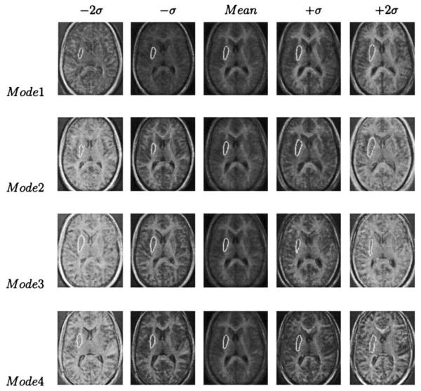
Fig. 1 shows a training set of left putamina in 12 MR brain images. By using multidimensional PCA, we can build a model of the shape-intensity profile of the left putamen. Fig. 2 illustrates the zero level sets and the associated intensities corresponding to the mean and four primary modes of variance of the distribution of the profile of the left putamen. Note that the mean shape-intensity pair and primary modes appear to be reasonable representations of the joint shape/intensity being learned.

Fig. 1.

Training set: outlines of left putamina in 12 2D MR brain images.

Fig. 2.

The four primary modes of variance of the left putamen and the image gray levels, showing the mean, ±SD (σ), and ±2σ.

We can also constrain the MAP estimation of 𝒮 by adding some regularizing terms (Chan and Vese, 2001; Tu and Zhu, 2002) into our active contour model: a general boundary smoothness prior, p_B(𝒮) = e^{−μ∮_𝒮 ds}, and a prior for the size of the region, p_A(𝒮) = e^−νAc, where A is the size of the region of object 𝒮, c is a constant and μ and ν are scalar factors. Here we assume the boundary smoothness and that the prior includes the size of the object. Thus, the joint prior probability p(𝒮, I) in Eq. (2) can be approximated by a product of the following probabilities:

$$p(𝒮,I)=p\left(\alpha \right)\cdot p_B\left(𝒮\right)\cdot p_A\left(𝒮\right).$$ (6)

Notice that the MAP estimation of the object in Eq. (2), 𝒮̂, is also the minimizer of the energy functional E shown below in the following equation:

$$\begin{array}{cc}\hfill E\left(𝒮\right)& =-\ln p(𝒮,I_{𝒮}\mid I)\propto -\ln [p(I\mid 𝒮,I_{𝒮})\cdot p(𝒮,I)]\hfill \\ \hfill & =-\ln [p(I\mid 𝒮,I_{𝒮})\cdot p\left(\alpha \right)\cdot p_B\left(𝒮\right)\cdot p_A\left(𝒮\right)]\hfill \\ \hfill & ={\lambda }_1\cdot {\int }_{(x,y,z)\text{inside}\left(𝒮\right)}{|I(x,y,z)-c_1|}^2\mathrm{d}x\mathrm{d}y\mathrm{d}z\hfill \\ \hfill & +{\lambda }_2\cdot {\int }_{(x,y,z)\text{outside}\left(𝒮\right),\text{inside}\left({\Omega }_{𝒮}\right)}{|I(x,y,z)-c_2|}^2\mathrm{d}x\mathrm{d}y\mathrm{d}z\hfill \\ \hfill & +\omega \cdot {\alpha }^{\mathrm{T}}{\Sigma }_k^{-1}\alpha +\mu {\oint }_{𝒮}\mathrm{d}s+\nu A^c.\hfill \end{array}$$ (7)

This minimization problem can be formulated and solved using the level set method (described in Section 2.3).

2.3. Level set formulation of the model

We will then minimize the energy functional E(𝒮) of shape 𝒮 in Eq. (7) using level sets. In the level set method, 𝒮 is the zero level set of a higher dimensional level set function ψ, i.e., 𝒮 = {(x, y, z)|ψ(x, y, z) = 0}. The evolution of the surface 𝒮 is given by the zero-level surface at time t of the function ψ(t, x, y, z). We define ψ to be positive outside 𝒮 and negative inside 𝒮.

For the level set formulation of our model, using the technique developed in (Chan and Vese, 2001), we replace 𝒮 with ψ in the energy functional in Eq. (7) using regularized versions of the Heaviside function H and the Dirac function δ, denoted by H_ε and δ_ε (Chan and Vese, 2001) (described below):

$$\begin{array}{cc}\hfill E\left(\psi \right)=& {\lambda }_1{\int }_{\Omega }{|I(x,y,z)-c_1|}^2[1-H_{\epsilon }\left(\psi (x,y,z)\right)]\mathrm{d}x\mathrm{d}y\mathrm{d}z\hfill \\ \hfill & +{\lambda }_2{\int }_{{\Omega }_{𝒮}}{|I(x,y,z)-c_2|}^2{H}_{\epsilon }\left(\psi (x,y,z)\right)\mathrm{d}x\mathrm{d}y\mathrm{d}z\hfill \\ \hfill & +\omega {\left(\left[\begin{array}{c}\hfill G\left(\psi \right)\hfill \\ \hfill G\left(I\right)\hfill \end{array}\right]-\overline{\left[\begin{array}{c}\hfill \Psi \hfill \\ \hfill I\hfill \end{array}\right]}\right)}^{\mathrm{T}}{U}_k{\Sigma }_k^{-1}{U}_k^{\mathrm{T}}\left(\left[\begin{array}{c}\hfill G\left(\psi \right)\hfill \\ \hfill G\left(I\right)\hfill \end{array}\right]-\overline{\left[\begin{array}{c}\hfill \Psi \hfill \\ \hfill I\hfill \end{array}\right]}\right)\hfill \\ \hfill & +\mu \int {\delta }_{\epsilon }\left(\psi (x,y,z)\right)|\nabla \psi (x,y,z)|\mathrm{d}x\mathrm{d}y\mathrm{d}z\hfill \\ \hfill & +\nu {\int }_{\Omega }[1-H_{\epsilon }\left(\psi (x,y,z)\right)]\mathrm{d}x\mathrm{d}y\mathrm{d}z,\hfill \end{array}$$ (8)

where Ω denotes the image domain. In our work, we define Ω_𝒮 to be the domain where the level set distance is no more than five pixels/voxels considering that the size of objects of interest in our data is less than 20–30 pixels/voxels, i.e., Ω_𝒮 = {(x, y, z)|ψ(x, y, z)≤5}, G(·) is an operator to form the column vector (as described in Section 2.2) of a matrix by column scanning. g(·) is the inverse operator of G(·). To compute the associated Euler–Lagrange equation for ψ, we minimize E with respect to ψ. Parametrizing the descent direction by artificial time t ≥ 0, the evolution equation in ψ(t, x, y, z) is

$$\begin{array}{cc}\hfill \frac{\partial \psi }{\partial t}=& {\delta }_{\epsilon }\left(\psi \right)\left\{{\lambda }_1{|I-c_1|}^2-{\lambda }_2{|I-c_2|}^2+\mu \cdot \mathrm{div}\left[\frac{\nabla \psi }{|\nabla \psi |}\right]+\nu \right\}\hfill \\ \hfill & -\omega \cdot g\left(U_{k1}{\Sigma }_k^{-1}\left[U_{k1}^{\mathrm{T}}(G\left(\psi \right)-\stackrel{-}{\Psi })+U_{k2}^{\mathrm{T}}(G\left(I\right)-\stackrel{-}{I})\right]\right)\hfill \end{array}$$ (9)

where U_k1 and U_k2 are the upper and lower half of the matrix U_k, respectively, i.e.,

$$\left[U_k\right]=\left[\begin{array}{c}\hfill U_{k1}\hfill \\ \hfill U_{k2}\hfill \end{array}\right].$$

2.4. Evolving the surface

We approximate H_ε and δ_ε as follows (Chan and Vese, 2001):

$$H_{\epsilon }\left(z\right)=\frac{1}{2}\left[1+\frac{2}{\pi }\arctan \left(\frac{z}{\epsilon }\right)\right],$$ (10)

$${\delta }_{\epsilon }\left(z\right)=\frac{\epsilon }{\pi ({\epsilon }^2+z^2)}.$$ (11)

The constants c₁ and c₂ are defined by (Yang et al., 2003)

$$c_1\left(\psi \right)=\frac{{\int }_{\Omega }I(x,y,z)\cdot [1-H\left(\psi (x,y,z)\right)]\mathrm{d}x\mathrm{d}y\mathrm{d}z}{{\int }_{\Omega }[1-H\left(\psi (x,y,z)\right)]\mathrm{d}x\mathrm{d}y\mathrm{d}z},$$ (12)

$$c_2\left(\psi \right)=\frac{{\int }_{{\Omega }_{𝒮}}I(x,y,z)\cdot H\left(\psi (x,y,z)\right)\mathrm{d}x\mathrm{d}y\mathrm{d}z}{{\int }_{{\Omega }_{𝒮}}H\left(\psi (x,y,z)\right)\mathrm{d}x\mathrm{d}y\mathrm{d}z}.$$ (13)

Given the surface ψ at time t, we seek to compute the evolution steps that bring the zero level set surface to the correct final segmentation based on the shape-intensity joint prior information and image intensity information. We first set up p(α) from the training set using PCA. At each stage of the algorithm, we recompute the constants c₁(ψ^t) and c₂(ψ^t), then upday ψ^t+1. This is repeated until convergence, i.e., until |ψ^t+1 − ψ^t| is small enough in our work.

The parameters λ₁, λ₂, μ, ν and ω are used to balance the influence of the shape-intensity joint prior model and the image information model. The tradeoff between joint prior and image information depends on how much faith one has in the joint prior model and the imagery for a given application. We set these parameters empirically for particular segmentation tasks, given the general image quality and the neighbor prior information. We define the parameters for applications in Section 4.

3. Evaluation of level set distribution models

As presented in Section 2.2, we use level sets as the representation of the object of interest in the image. The shape-intensity joint distribution model is approximated by the joint distribution of the level set function of the object shape and the image gray levels. To analyze the performance of this level set approximation of the object shape in the joint prior model, we can evaluate the level set distribution model (LSDM) presented in (Leventon et al., 2000; Tsai et al., 2001, 2003a; Yang et al., 2003), where the LSDM is used as an approximation of the distribution of the object shape. Since the level set function is a nonlinear function of the corresponding zero level set (i.e. the surface of the object), it is very difficult to theoretically analyze the performance of the LSDM as an approximation of the shape model. A practical way to evaluate it is to compare the LSDM with the point distribution model (PDM) (Cootes et al., 1994).

In a PDM, each shape is represented by a set of points on the boundary. The labeling of the points is important. Each point represents a particular part of the object boundary, so it must be located in the same way on each of the training images, which can be difficult for 3D objects. Let X_i = (x_i1, y_i1, X_i2, y_i2, …, X_iL, y_iL)^T be a vector describing the set of L points of the ith shape in the set. (x_ij, y_ij) is the jth point of the ith shape. Table 1 shows the PCA processes of getting the LSDM and PDM over a set of n aligned training images.

Table 1.

Level set distribution model (LSDM) and point distribution model (PDM)

	LSDM	PDM
Shape representation	{Ψ1, Ψ2, …, Ψn}, Ψi : Nd elements	{X1, X2, …, Xn}, Xi : dL elements
Mean shape	$\stackrel{-}{\Psi }=(1∕n){\Sigma }_{i=1}^n{\Psi }_i$	$\stackrel{-}{X}=(1∕n){\Sigma }_{i=1}^n{X}_i$
Mean offset matrix	QΨ	QX
SVD	$Q_{\Psi }=U_{\Psi }{\Sigma }_{\Psi }{V}_{\Psi }^{\mathrm{T}}$	$Q_X=U_X{\Sigma }_X{V}_X^{\mathrm{T}}$
Parametric model	Ψ̃ = Ψ̄ + UΨ,kαΨ	X̃ = X̄ + UX,kαX
Probability of shape	$p\left({\alpha }_{\Psi }\right)=\frac{1}{\sqrt{{\left(2\pi \right)}^k\left|{\Sigma }_{\Psi ,k}\right|}}\cdot \exp \left[-\frac{1}{2}{\alpha }_{\Psi }^{\mathrm{T}}{\Sigma }_{\Psi ,k}^{-1}{\alpha }_{\Psi }\right]$	$p\left({\alpha }_X\right)=\frac{1}{\sqrt{{\left(2\pi \right)}^k\left|{\Sigma }_{X,k}\right|}}\cdot \exp \left[-\frac{1}{2}{\alpha }_X^{\mathrm{T}}{\Sigma }_{X,k}^{-1}{\alpha }_X\right]$

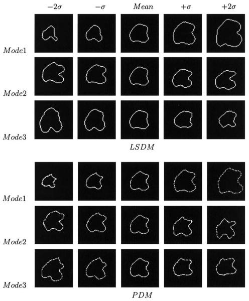
By performing PCA on the level set functions of the left ventricles in Fig. 3, we can build a model of the shape of left ventricles. The top of Fig. 4 illustrates zero level sets corresponding to the mean and three primary modes of variance of the distribution of the level set of the left ventricle. Note that the zero level sets of the mean level set and primary modes appear to be reasonable representative shapes of the class of object being learned. The bottom of Fig. 4 shows the three PDM-based primary modes of variance of the left ventricle using the same training set as in Fig. 3, where the correspondences between the boundary points were manually determined. Compared to the PDM, the zero level set tends to have a smoother boundary over the distribution. The two models are quite similar in describing the main variations of the left ventricle endocardial border.

Fig. 3.

Outlines of left ventricles in 6 out of 16 2D MR training images gated and at a fixed point in the cardiac cycle.

Fig. 4.

The three primary modes of variance of the left ventricle using level set (top rows) and point (bottom rows) model, showing the mean, ±SD (σ), and ±2σ.

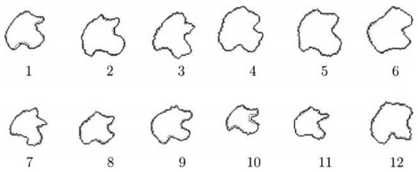
We then estimate a number of test left ventricles using the parametric models of LSDM and PDM as shown in Table 1. Fig. 5 shows the two estimates of 12 manually segmented left ventricles (with 5 primary modes). Most parts of the two curves overlap well. To compare the two estimates, using the same measure used in (Leventon et al., 2000), we compute the undirected Hausdorff distance (Huttenlocher et al., 1993) between the zero level set 𝒜 (N_𝒜 points) and the sample points ℬ

$$H(𝒜,ℬ)=\max (h(𝒜,ℬ),h\left(\right(ℬ,𝒜)),$$ (14)

where

$$h(𝒜,ℬ)=\frac{1}{N_{𝒜}}\underset{a\in 𝒜}{\Sigma }\underset{b\in ℬ}{\min }\parallel a-b\parallel .$$ (15)

The distances of the LSDM and PDM based estimates for the 12 cases in Fig. 5 are shown in Table 2 (unit: pixel). Virtually all the points in the zero level set lie within one or two pixels of the PDM estimate.

Fig. 5.

Level set distribution model (green) and point distribution model (red) based estimates for 12 test left ventricles. The estimates are obtained from the parametric models shown in Table 1. (For interpretation of the reference to color in this figure legend, the reader is referred to the web version of this article.)

Table 2.

Hausdorff distance between the LSDM and the PDM estimates in Fig. 5

Example	1	2	3	4	5	6	7	8	9	10	11	12
Distance	2.1	1.8	1.3	0.9	1.1	0.9	0.8	1.9	1.4	2.0	1.5	1.6

(unit: pixel).

Next, we evaluate the two distributions p(α_ψ) and p(α_X) in Table 1 by doing a χ² test, again using the left ventricle as the example. Since the PDM based p(α_X) is built in the sample point vector space, while the LSDM based p(α_ψ) is in the level set space, we need to convert the two distributions in the same space first in order to do the comparison. We first randomly generate a set of samples {X₁, X₂, …, X_m, m = 10⁵} (each sample corresponds to a shape represented by a sample point vector) based on the PDM p(α_X). Each X_i can be embedded as the zero level set of a higher dimensional level set function ψ_i, the projection of X_i in the level set space. Then we compare the set of projections {ψ₁, ψ₂, …, ψ_m, m = 10⁵} with the LSDM p(α_ψ) using the χ² test, with the null hypothesis, H₀, that the projections {ψ₁, ψ₂, …, ψ_m, m = 10⁵} have the same distribution defined by the LSDM p(α_ψ). Consider the first five principal components in the LSDM, with five bins along each of the principal modes, the χ₂ statistic is given by

$${\chi }^2=\Sigma \frac{{(\mathrm{Ob}.-\mathrm{Ex}.)}^2}{\mathrm{Ex}.},$$ (16)

where the sum is over all the bins considered, Ob. is the observed frequency of ψ_𝒮 falling in each bin, Ex. is the corresponding expected frequency which can be calculated by integrating the LSDM probability function p(α_ψ) in Table 1 over the bin. For our test ((5 − 1)⁵ = 1024 degrees of freedom), χ² = 981, with an upper tail probability Pr(χ² > 981) = 0.82. Therefore, there is a 0.82 probability that it is wrong to reject H₀. Thus, the two distributions are statistically indistinguishable.

The level set representation of object shape is an efficient way to formulate a distribution model for both 2D and 3D objects, and appears to be an accurate approximation to the corresponding PDM. Moreover, it does not require explicit point correspondences (since the shape is embedded in a level set function).

4. Experimental results

We have used our model on various medical images. To simplify the complexity of the segmentation system, we generally choose the parameters in our experiments as follows: λ₁ = λ₂ = λ, μ = 0.00005 × 255², ν = 0 (Chan and Vese, 2001). This leaves us only two free parameters (λ and ω) to balance the influence of two terms, the image data term and the shape-intensity joint prior term. We rigidly align the training data before performing PCA. All the tested images are not in their training sets.

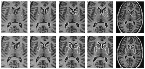
We first consider a 2D MR brain image with eight sub-cortical structures of different intensities and with blurred boundaries. The top of Fig. 6 shows a few steps of the segmentation using only gray level information. Only the lower (posterior) portions of the lateral ventricles can be segmented perfectly since they have clearer boundaries. The bottom of Fig. 6 shows the results of using our shape-intensity joint prior model, the training set model of the left putamen is shown in Figs. 1 and 2. The curves are able to converge on the desired boundaries even though some parts of the boundaries are too blurred to be detected using only gray level information. The segmentation converges in 2 min on a 2.00 GHz Intel XEON CPU.

Fig. 6.

Four steps of the segmentation of eight sub-cortical structures (the lateral ventricles (λ = 0.9, ω = 0.1), heads of the caudate nucleus (λ = 0.3, ω = 0.7), and putamina (λ = 0.2, ω = 0.8)) in a 2D MR brain image without prior information (top) and with shape-intensity joint prior (bottom). The training set consists of 12 MR images shown in Fig. 1.

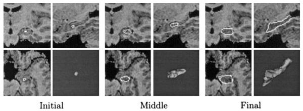
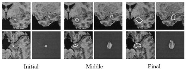
We then test our method using 3D images. Fig. 7 shows a few steps in the segmentation of the left hippocampus in a MR brain image. Fig. 8 illustrates three steps in the segmentation of the left amygdala. Segmenting the two structures can be very tough without using prior information since both structures have very poorly defined boundaries. After using our shape-intensity joint prior model, as shown in Figs. 7 and 8, the two structures can be clearly segmented. Segmenting these 3D images (with size 172×148×124) took less than an hour.

Fig. 7.

Segmentation of the left hippocampus. Three orthogonal slices and the 3D surfaces are shown for each step. The training set consists of 12 MR images λ = 0.1, ω = 0.9.

Fig. 8.

Segmentation of the left amygdala. Three orthogonal slices and the 3D surfaces are shown for each step. The training set consists of 12 MR brain images. λ = 0.1, ω = 0.9.

To validate the segmentation results, we test our model on 12 different images for each of the above three cases (Figs. 6-8), respectively. Here we use the “leave-one-out” experiments, where each test image is segmented using the rest 11 images as the training set. We then compute the undirected Hausdorff distance of pixels between the boundary of the computed segmentation and the boundary of the manual segmentation using Eqs. (14) and (15). For our experiments, the mean distances show improvement in all the three cases comparing with/without the shape-intensity joint prior, as seen in Table 3. Virtually all the boundary points obtained using our model lie within one; or two voxels of the manual segmentation.

Table 3.

Mean distance between the computed and the manual boundaries

	Sub-cortical structures	Hippocampus	Amygdala
Without joint prior	9.2	11.2	5.8
With joint prior	2.0	1.8	1.6

(unit: mm).

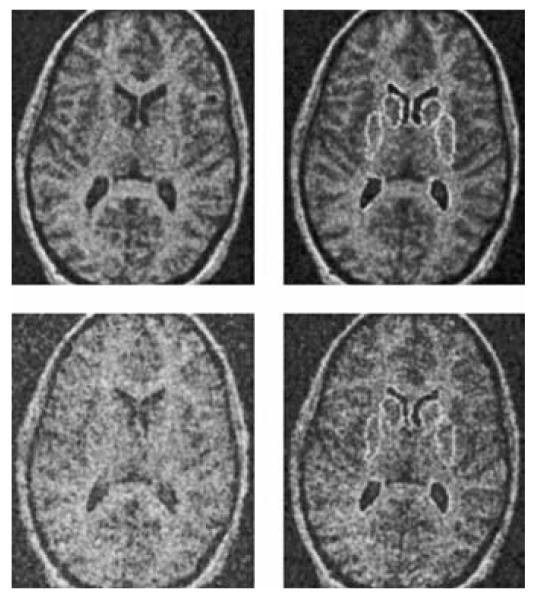
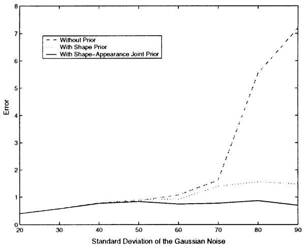
We also test the robustness of our algorithm to noise. We add Gaussian noise with different variances to the MR image in Fig. 6 (the mean intensities of white/gray matters: 45/65), then segment it. Fig. 9 shows the segmentation results with Gaussian noise of SD of 20 (top) and 40 (bottom). Fig. 10 shows the segmentation error of the lower portion of the left lateral ventricle in three cases: with no prior, with shape prior, and with shape-intensity joint prior. As the variance of the noise increases, the error for no prior increases rapidly since the structure is too noisy to be detected using only gray level information. However, for shape prior and shape-intensity joint prior methods, the errors are much lower and are locked in a very small range even when the variance of the noise is very large. Note that our shape-intensity joint prior model achieves the least error among all the cases.

Fig. 9.

Original and segmented images with Gaussian noise of σ = 20 (top) and 40 (bottom).

Fig. 10.

Segmentation errors (unit: mm) with different variances of Gaussian noise for the MR images in Fig. 6 (the mean intensities of white/gray matters: 45/65).

5. Discussion and conclusions

In this paper, we present a MAP estimation framework based model for image segmentation using shape-intensity joint prior information. We introduce a representation for the shape-intensity joint density function, and define joint probability distribution over the variations of the shape-intensity pair in a set of training images. We estimate the MAP shape of the object using evolving level set based on the associated Euler–Lagrange equation. From various experiments on 2D and 3D medical images, we have demonstrated that our model is able to handle multidimensional data and robust to noise. This approach can be used to segment images with poor image contrast, noise, and missing or diffuse boundaries.

The image term we used (Eq. (3)) has been mainly used for the segmentation of structures with homogeneous intensities inside the objects, and may be enhanced. For instance, it would be interesting to extend the image gray level based model to a more general case where additional information is included besides the image intensity average, as has been discussed (Chan and Vese, 2001). More segmentation examples using similar image term have been provided in (Chan and Vese, 2001).

We evaluate the LSDM by comparing it with the traditional PDM. For the endocardial boundary representations shown in Section 3, it is clear that either representation would be acceptable even though they are slightly different. Both models can be used as approximations to the distribution of object shape.

By using the level set representation of the shape, we avoid the need for explicit point correspondences during the training phase. Level set representation of object shape provides tolerance to slight misalignment of object shape, in the attempt to avoid having to solve the general correspondence problem. In practice, the variations captured by the principal components in LSDM in this paper are based on rigid alignment of the training data and may contain undesired residuals due to misalignment. We are looking for better alignment method that can reduce such residuals and the undesired topology problem.

As a powerful approach to deformable models, the MAP framework can combine prior information and given image information to realize image segmentation. While we have not pursued in this paper, a more unified model could be used to incorporate shape priors, neighbor constraints (Yang et al., 2002, 2003; Yang and Duncan, 2004) as well as image intensity priors (Yang and Duncan, 2003).

References

- Caselles V, Catte F, Coll T, Dibos F. A geometric model for active contours in image processing. Numer. Math. 1993;66:1–31. [Google Scholar]
- Caselles V, Kimmel R, Sapiro G. Geodesic active contours. Int. J. Comput. Vis. 1997;22(1):61–79. [Google Scholar]
- Chan T, Vese L. Active contours without edges. IEEE Trans. Image Process. 2001;10(2):266–277. doi: 10.1109/83.902291. [DOI] [PubMed] [Google Scholar]
- Chen Y, Tagare H, Thiruvenkadam S, Huang F, Wilson D, Gopinath KS, Briggs RW, Geiser EA. Using prior shapes in geometric active contours in a variational framework. Int. J. Comput. Vis. 2002;50(3):315–328. [Google Scholar]
- Cootes T, Beeston C, Edwards G, Taylor C. A unified framework for atlas matching using active appearance models. Inf. Process. Med. Imaging (IPMI) 1999 [Google Scholar]
- Cootes T, Edwards G, Taylor C. Active appearance models. IEEE Trans. Pattern Anal. Mach. Intell. 2001;23(6):681–685. [Google Scholar]
- Cootes TF, Hill A, Taylor CJ, Haslam J. Use of active shape models for locating structures in medical images. Image Vis. Comput. 1994;12(6):355–365. [Google Scholar]
- Davies RH, Twining CJ, Cootes TF, Waterson JC, Taylor CJ. A minimum description length approach to statistical shape modelling. IEEE Trans. Med. Imaging. 2002;21(5):525–537. doi: 10.1109/TMI.2002.1009388. [DOI] [PubMed] [Google Scholar]
- Huttenlocher D, Klanderman G, Rucklidge W. Comparing images using the Hausdorff distance. IEEE Trans. Pattern Anal. Mach. Intell. 1993;15(9):850–863. [Google Scholar]
- Kass M, Witkin A, Terzopoulos D. Snakes: active contour models. Int. J. Comput. Vis. 1987;1:321–331. [Google Scholar]
- Leventon M, Grimson E, Faugeras O. Statistical shape influence in geodesic active contours. IEEE Conf. Comput. Vis. Pattern Recog. 2000;1:316–323. [Google Scholar]
- Malladi R, Sethian JA, Vemuri BC. A topology independent shape modeling scheme. Proc. SPIE Conf. Geometric Methods Comput. Vis. II. 1993;2031:246–258. [Google Scholar]
- Osher S, Sethian JA. Fronts propagating with curvature-dependent speed: algorithms based on Hamilton–Jacobi formulation. J. Comput. Phy. 1988;79:12–49. [Google Scholar]
- Staib L, Duncan J. Boundary finding with parametrically deformable models. IEEE Trans. Pattern Anal. Mach. Intell. 1992;14(11):1061–1075. [Google Scholar]
- Styner M, Rajamani K, Nolte LP, Zsemlye G, Szekely G, Taylor C, Davies RH. Evaluation of 3D correspondence methods for model building. Inf. Process. Med. Imaging. 2003:63–75. doi: 10.1007/978-3-540-45087-0_6. [DOI] [PubMed] [Google Scholar]
- Tsai A, Yezzi A, Wells W, Tempany C, Tucker D, Fan A, Grimson E, Willsky A. Model-based curve evolution technique for image segmentation. IEEE Conf. Comput. Vis. Pattern Recog. 2001;1(December):463–468. [Google Scholar]
- Tsai A, Yezzi A, Wells W, Tempany C, Tucker D, Fan A, Grimson E, Willsky A. A shape-based approach to curve evolution for segmentation of medical imagery. IEEE Trans. Med. Imaging. 2003a;22(2):137–154. doi: 10.1109/TMI.2002.808355. [DOI] [PubMed] [Google Scholar]
- Tsai A, Wells W, Tempany C, Grimson E, Willsky A. Coupled multi-shape model and mutual information for medical image segmentation. Inf. Process. Med. Imaging. 2003b;(July):185–197. doi: 10.1007/978-3-540-45087-0_16. [DOI] [PubMed] [Google Scholar]
- Tu Z, Zhu S. Image segmentation by data-driven Markov chain Monte carlo. IEEE Trans. Pattern Anal. Mach. Intell. 2002;24(5):657–673. [Google Scholar]
- Wang Y, Staib LH. Boundary finding with correspondence using statistical shape models; IEEE Conference on Computer Vision and Pattern Recognition (CVPR'98); Santa Barbara, CA, USA. 1998. pp. 338–345. [Google Scholar]
- Yang J, Duncan J. 3D image segmentation of deformable objects with shape-appearance joint prior models. Medical Image Computing and Computer-Assisted Intervention (MICCAI) 2003;1:573–580. [Google Scholar]
- Yang J, Duncan J. Joint prior models of neighboring objects for 3D image segmentation; IEEE Computer Society Conference on Computer Vision and Pattern Recognition (CVPR); 2004. pp. 314–319. [DOI] [PMC free article] [PubMed] [Google Scholar]
- Yang J, Staib L, Duncan J. Statistical neighbor distance influence in active contours. Medical Image Computing and Computer-Assisted Intervention (MICCAI) 2002;1:588–596. [Google Scholar]
- Yang J, Staib L, Duncan J. Neighbor-constrained segmentation with 3D deformable models. In: Taylor CJ, Noble JA, editors. Lecture Notes in Computer Science, IPMI; 18th International Conference on Information Processing in Medical Imaging; Springer, Berlin. 2003. pp. 198–209. [DOI] [PubMed] [Google Scholar]
- Yang J, Staib L, Duncan J. Neighbor-constrained segmentation with level set based 3D deformable models. IEEE Trans. Med. Imaging. 2004 doi: 10.1109/TMI.2004.830802. in press. [DOI] [PMC free article] [PubMed] [Google Scholar]
- Yezzi A, Tsai A, Willsky A. A statistical approach to snakes for bimodal and trimodal imagery; Seventh IEEE International Conference on Computer Vision.1999. pp. 898–903. [Google Scholar]
- Zeng X, Staib LH, Schultz RT, Duncan JS. Segmentation and measurement of the cortex from 3D MR images using coupled surfaces propagation. IEEE Trans. Med. Imaging. 1999;18(10):100–111. doi: 10.1109/42.811276. [DOI] [PubMed] [Google Scholar]