

Abstract
Sufficient temporal resolution is required to image the dynamics of blood flow, which may be critical for accurate diagnosis and treatment of various intracranial vascular diseases, such as arteriovenous malformations (AVMs) and aneurysms. Highly-constrained projection reconstruction (HYPR) has recently become a technique of interest for high-speed contrast-enhanced magnetic resonance angiography (CE-MRA). HYPR provides high frame rates by preferential weighting of radial projections while maintaining signal-to-noise ratio (SNR) by using a high SNR composite. An analysis was done to quantify the effects of HYPR on SNR, contrast-to-noise ratio (CNR), and temporal blur compared to the previously developed radial sliding-window technique using standard filtered backprojection or regridding methods. Computer simulations were performed to study the effects of HYPR processing on image error and the temporal information. Additionally, in vivo imaging was done on patients with angiographically confirmed AVMs to measure the effects of alteration of various HYPR parameters on SNR as well as the fidelity of the temporal information. The images were scored by an interventional radiologist in a blinded read and were compared with X-ray digital subtraction angiography (DSA). It was found that with the right choice of parameters, modest improvements in both SNR and dynamic information can be achieved as compared to radial sliding-window MRA.
Keywords: HYPR, radial imaging, MRA, time-resolved, arteriovenous malformation, AVM
Contrast-enhanced MR angiography (CE-MRA) (1) has been a successful clinical imaging modality. The successful translation of CE-MRA into the day-to-day diagnosis of vascular disease depends on the work of several individuals and groups (2–14). In CE-MRA, high signal-to-noise ratio (SNR) and spatial resolution are desired to visualize small arteries. At the same time, sufficient temporal resolution is required to image the dynamics of the blood flow, which may be critical for accurate diagnosis and treatment of various vascular diseases, such as arteriovenous malformations (AVMs) and aneurysms.
Despite the success of CE-MRA in many vascular beds, X-ray digital subtraction angiography (DSA) remains the current clinical standard for time-resolved angiography of the intracranial vasculature, although it is invasive and has ionizing radiation and nephrotoxic contrast agents. X-ray DSA has spatial and temporal resolution superior to MRA, typically with a frame rate of three to six frames per second. Such temporal resolution is required to image a number of neurovascular conditions, including intracranial AVMs (IAVMs), which affect the lives of up to 300,000 people between the ages of 20 and 40 years in the United States alone (15). The treatment of IAVMs is complex; it must be tailored (16,17) to each patient and monitored with periodic angiograms. One approach, radioembolization using gamma knife surgery, must be planned using an X-ray angiogram acquired at peak nidal enhancement prior to venous opacification. The demands of a high frame rate and high spatial resolution present a challenge to current methods of performing CE-MRA.
There have been many improvements to CE-MRA in increasing the temporal resolution. To accelerate the speed of acquisition, partial Fourier (13,18) can be used, where only parts of the k-space are acquired. Further acceleration can be achieved by parallel imaging (19–23), where multiple receiver coils are used in parallel to each acquire different information. Cashen et al. (24) proposed radially sampling (25,26) of k-space with a sliding window reconstruction to increase the frame rate of CE-MRA. Based on the early work of Riederer et al. (2), this technique reconstructs intermediate frames between repeated measurements so that time-resolved series of images can be updated as often as the time it takes to acquire one radial projection. In comparison to X-ray, the MRA still has a higher artifact level and inferior SNR, and suffers from temporal blurring due to the lengthy acquisition time, or broad “temporal footprint,” of the acquisition of 3D data sets.
An alternative approach to dynamic imaging was recently proposed by Mistretta et al. (27). Highly-constrained projection reconstruction (HYPR) can achieve high frame rates by reconstructing sparse k-space data combined with a high-SNR composite image (27,28). HYPR requires the data to be sparse in space and there is ongoing debate as to the fidelity of the dynamic information (29) owing to the broad temporal footprint of the composite image. The interaction between the sparsity of the image data, the temporal footprint of the composite image, and the fidelity of the dynamic information is an area of active research (27,29).
We hypothesized that HYPR processing yields significant improvements in SNR compared to radial sliding window reconstruction without HYPR processing. We also hypothesized that the portrayal of dynamic information in HYPR depends upon specific aspects of the HYPR data selection. We evaluated our approach using composite images with broad and narrow temporal footprints as well as time frames of varying sizes. Our studies were performed using computer simulations and angiographically confirmed intracranial AVM patients. Furthermore, MRA images were clinically evaluated by a radiologist through direct comparison with X-ray angiography in patients with intracranial AVMs.
Materials and Methods
We performed the simulations, acquisitions, and HYPR processing based on a pulse sequence that uses a radial k-space trajectory in-plane and Cartesian sampling through-plane, also known as the “stack of stars” sampling scheme (24). We coupled this acquisition with a sliding window reconstruction to allow frame rates comparable to intracranial X-ray angiography.
HYPR
The original HYPR image reconstruction algorithm developed by Mistretta et al. (27) uses the following formula:
| [1] |
The HYPR image, IHYPR(x,y,z), is calculated by multiplying the time-averaged composite C(x,y.z) with an image reconstructed using the ratio of unfiltered backprojections (BPs) of the current time frame P(r,θ,φ) and corresponding unfiltered backprojections of the composite image PC(r,θ,φ). P(r,θ,φ) usually consists of limited projections, a small subset of the full number of projections covering 180°. Then, the image intensity is scaled by dividing the limited number of projections, NP (a subset of full Nθ projections), used to reconstruct each time frame. Huang and Wright (29) have proposed the following correction to the original formula (Eq. [1]):
| [2] |
With the correction, IHYPR(x,y,z) converges to the composite image C(x,y,z) when the number of limited projections, NP, approaches the number of projections used to make the composite, since ΣP(r,θ,φ)/ΣPC(r,θ,φ) = 1.
The corrected formula (Eq. [2]) was used in this study. However, in our study, to maximize the SNR in HYPR images, we signal-averaged the composite, C(x,y,z), over multiple measurements of the 3D volume where contrast agent was present (static composite). The composite was also formed by time averaging a number of projections before and after the current frame (sliding composite). Figure 1 illustrates the two composites. In either case, ΣP(r,θ,φ)/ΣPc(r,θ,φ) does not equal one, and for NP equal to the number of projections in the composite, the HYPR image is not the same as the composite image. The composite, which also has Nθ projections, is time averages of multiple repetitions containing Nθ projections.
FIG. 1.
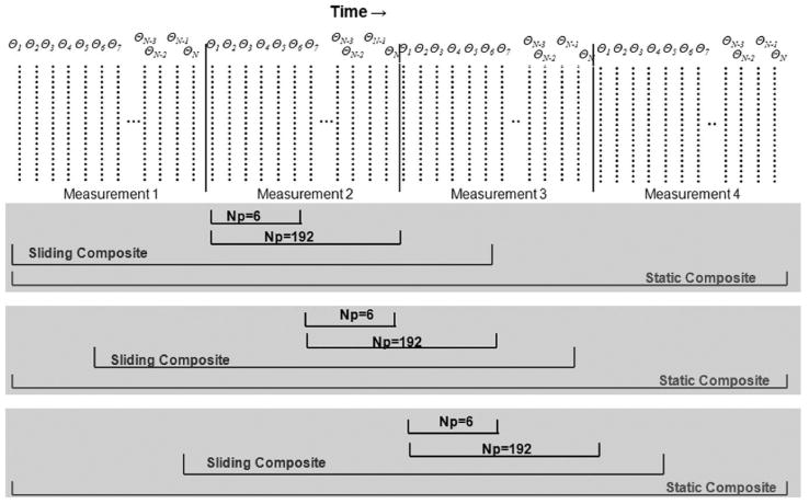
Timing diagram of HYPR with sliding and static composites. The sliding composite slides along each set of limited projections, while the static composite stays fixed for each frame. The radial projections (dotted vertical lines) indicated by θN, where N is the pseudorandom acquisition order.
The NP indicates the number of in-plane projections. With a 3D or multislice acquisition, the NP includes all the projections with the same angle in that 3D volume. Hence, throughout the remainder of this work, it should be understood that when NP is stated as being a specific number of projections, the actual number of projections included in the image is NP times the number of slice or partition encodings.
Simulations
Computer simulations were performed in order to quantify the effects of HYPR processing on temporal profiles of contrast bolus, as well as image artifacts. By doing computer simulations we were able compare how each reconstruction method alters the truth images. Unlike in vivo imaging, the truth images can be user-defined. This allows a known input to HYPR processing, enabling direct comparison of the effects of HYPR on the truth images.
All simulations were performed using MATLAB (V2006b; The Mathworks, Natick, MA, USA). A simulation model was adopted from a previous study (24) that modeled a bolus of contrast agent using a 3D step function moving in a straight line across the field of view (FOV) over time (Fig. 2). This geometry was chosen because the functions can be modeled as a product of three separable rect functions in the x, y, and z dimensions, and can be analytically transformed back and forth in k-space and image space so that k-space sampling can be done on the true k-space representation of the truth images. The image space function for the bolus moving from left to right (L-R) can be represented as follows:
FIG. 2.
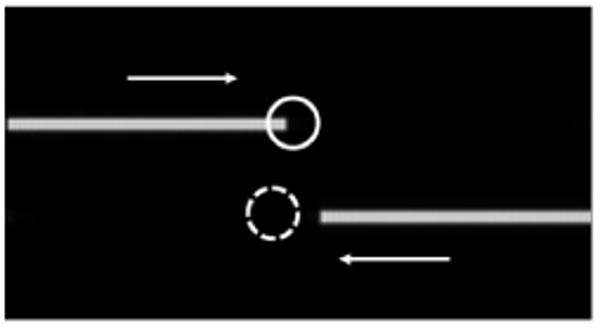
Simulation truth image and ROIs that represent artery (solid) and vein (dotted). The length of these objects increases over time in the direction of the arrows to simulate arterial and venous filling.
| [3] |
Equation [3], when transformed into rectangular k-space, becomes
| [4] |
where w is the thickness of the vessel, v is the velocity of moving bolus flowing through a blood vessel, and t is time in seconds. This effectively models a step function moving in the y direction. The cylindrical representation can be obtained by substituting kx = kr sin (kθ) and kx = kr cos (kθ). The analytical function in k-space (product of sinc functions) was sampled radially with real imaging parameters. Gaussian noise with standard deviation (SD) equal to the maximum value of I(kx,ky,kz,t) divided by 300 was added to the k-space simulation data to yield a maximum SNR of 300 for each projection. The truth images were defined as the inverse Fourier transform of the k-space function for a case where t is a discrete variable for each measurement volume, which simulates an infinitely short acquisition time.
Simulations were performed with two 4-pixel-thick bolus models with one bolus moving from left to right at 7 mm/s in a 250 mm × 250 mm × 32 mm pixel FOV, and the other moving in the opposite direction at the same speed. The simulated data sampling was based on our clinical 3D radial MRA sequence with the following parameters: TR = 3 ms, NSlices = 16, slice thickness = 2 mm, number of angles (Nθ) = 192, NReadout = 192, and NRepetitions = 8. The data were reconstructed using conventional filtered BP with sliding window with full 192 projections, as well as using HYPR with projections NP = 6, 16, 32, 64, and 192, which includes all the partitions for those projections. A sliding window factor of 32 was used for all reconstructions, so that 32 intermediate images were obtained between each volume repetition. The static composite for the HYPR reconstruction was obtained by averaging all eight repetitions reconstructed with filtered BP of full 192 projections without sliding window. The sliding composite was formed by filtered BP of the time average of 192 projections behind the first frame and 96 projections after the current frame.
To quantify the artifact level of the images, reconstructed image error was measured as a function of the reconstructed time frame throughout the bolus passage. Simulations done without added Gaussian noise were used for the artifact level calculation to calculate pure artifact without noise. Image errors of the HYPR processed images were calculated using a modification of an established method (30). The formula used to calculate image error is:
| [5] |
For HYPR, additional energy is introduced to the image from the composite. Therefore, subtraction from the truth must be done after appropriate normalization. For our studies, all images were normalized so that the total energy for a single image is one. Then Σx,y[Itruth(x,y)]2 = 1, and Eq. [5] reduces to:
| [6] |
The average and SD of image errors were calculated for each number of projections used. A paired Student's t-test was performed to compare the static and sliding composites.
Regions of interest (ROIs) were selected in the simulation images and intensity was plotted over time on images with added noise. The chosen ROIs are shown on Fig. 2. The ROIs were chosen in such a way that one represents an arterial time course and the other represents a venous time course. The plots were normalized so that the maximum value of the intravascular signal was one. SNR was also calculated by averaging the value inside the ROIs and dividing by the SD of the values inside an ROI covering a region of the simulation where no signal should be present.
AVM Patient Studies
We tested the simulated results by scanning four patients with angiographically confirmed AVMs. The imaging protocols were approved by the institutional review board (IRB).
Sequence
Images were acquired with a Siemens 3T Trio scanner (Siemens Medical Solutions, Erlangen, Germany) and a 3D spoiled gradient-echo sequence with a radial in-plane and Fourier through-plane trajectory. The partition loop was inside the projection loop. Signal reception was provided by a receive-only 12-channel head coil. Typical imaging parameters were: FOV = 220 mm × 220 mm, partition thickness = 2.5 mm, TR = 2.7–3.0 ms, TE = 1.3 ms, Nθ = 128 or 192, NReadout = 192, NSlices = 20–30, readout/slice partial Fourier factors = 75%/75%, receiver bandwidth = 1300 Hz/pixel, and flip angle = 15°. Images were acquired in a sagittal plane with z-phase encoding in the L-R direction. The resulting acquisition was 1.15 mm × 1.15 × 2.5 mm. With the parameters above, the resulting in acquisition times were between 7 and 13 s per repetition. The number of repetitions was varied so that the total imaging time was close to 90 s. To minimize the coherence of undersampling artifacts, the radial projections were acquired in a pseudorandom order instead of linearly increasing the angle from 0° to 180° using the scheme described (24).
A single dose (0.1 mmol/kg) of Gd-DTPA (Magnevist; Berlex, Wayne, NJ, USA) was administered for each scan with a power injector (Spectris Solaris; MEDRAD, Indianola, PA, USA). The images were acquired in a sagittal and/or coronal plane. For sagittal scans, the z encoding was done in the L-R direction, and for coronal scans, the z encoding was done in the anterior–posterior direction. When images were taken from both sagittal and coronal planes, the order of acquisition was randomized to reduce the effect of residual gadolinium in the first scan.
Reconstruction
Raw data were obtained from the scanner for reconstruction using MATLAB. A Fourier transform was performed in the z and r dimensions. The first measurement volume, acquired prior to contrast agent administration, was then subtracted from the later frames. Then filtered BP and HYPR processing was performed using both static and sliding composites. Similarly to the reconstruction done with simulation data, a sliding window factor of 32 was used. This resulted in 32 intermediate frames between actual measurements and reconstructed frame rate of 3.2 frames/s. The sliding composite was set by averaging projections measured 10 s (192 projections) behind and 5 s (96 projections) ahead of the current frame. Finally, maximum intensity projections (MIPs) were obtained from the 3D volume images.
Analysis
ROIs were drawn on the MIPs to cover the common carotid and the superior sagittal sinus on sagittal images to serve as representative regions of arterial and venous enhancement, respectively. To calculate the SNR, the values inside the ROIs were averaged and divided by the SD of an ROI drawn in the air.
Temporal profiles were plotted by taking the average of values inside each ROI as a function of time. The overlap integral was used to quantify the separation of arterial and venous phases. In a sense, it evaluates the degree of venous contamination. The overlap integral is defined as:
| [7] |
where A[n] and V[n] are temporal profiles normalized so that their maximum value is one. It simply calculates the area of the region of overlap between arterial and venous curves in the temporal profiles. A lower overlap integral corresponds to better separation between arterial and venous phases.
The quality of the MRA images of the intracranial AVMs was scored by an interventional radiologist blinded to the reconstruction parameters. The clinician was given reconstruction sets that varied in NP and composite type in a random order. The image quality was given scores (1 = nondiagnostic, 2 = poor, 3 = good, and 4 = excellent) in the following categories: visualization of feeders, visualization of nidus, visualization of draining veins, SNR/artifacts, and quality of dynamic information. The scores were given relative to the X-ray DSA images, the standard of reference.
Results
Simulations
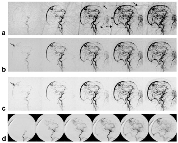
Figure 3 shows five sets of reconstructed time frames from the simulation of bolus dynamics with each frame separated by 12 frames (3.6 s). Figure 3a represents truth images. Figure 3b and c show HYPR reconstruction using only six projections with sliding and static composites, respectively. Similarly, Fig. 3d and e were reconstructed using 192 projections with sliding and static composites, respectively. Figure 3f is a filtered BP with 192 projections without HYPR, which has been included for reference. HYPR reconstruction with only six projections results in misrepresentation of the simulated bolus (see arrows in Fig. 3b and c). The first frame of Fig. 3c, where the length of the bolus should be the shortest, shows a longer bolus profile than the later frames. While the sliding composite image (Fig. 3b) exhibits a better representation of the true extent of the simulated bolus, the first frame still shows an artifact that makes the bolus look longer. The artifacts in the direction of movement for HYPR images, which appear randomly in consecutive frames not included in the figures, are reduced as more projections are used, as shown in Fig. 3d (also see Table 1), but the front end of the bolus is spatially elongated for every frame, more severely for the static composite. When 192 projections are used for HYPR, the sliding composite images more closely resemble the filtered BP without HYPR, as well as truth images, than static composite images.
FIG. 3.
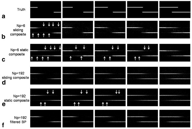
Comparison of HYPR reconstruction using small and large numbers of projections with static and sliding composites. In each set of images the time frame increases from left to right, with frames separated by 1.5 s in time. a: Truth. b: Sliding composite HYPR (NP = 6). c: Static composite HYPR (NP = 6). d: Sliding composite HYPR (NP = 192). e: Static composite HYPR (NP = 192). f: Filtered BP without HYPR reconstruction. Arrows indicate misrepresentation of the bolus model.
Table 1.
Image Error and SNR Over Time for Varying Number of Projections in HYPR*
| Number of projections | Average image error | SD image error | Average SNR | |||
|---|---|---|---|---|---|---|
| Static composite | Sliding composite | Static composite | Sliding composite | Static composite | Sliding composite | |
| 6 | 34.6 | 34.3 | 8.88 | 6.64 | 24.2 | 15.5 |
| 16 | 32.1 | 31.6 | 4.66 | 2.96 | 24.4 | 15.4 |
| 32 | 33 | 30.9 | 3.97 | 2.94 | 25.1 | 16.8 |
| 64 | 35.2 | 31.6 | 3.19 | 3.27 | 25.7 | 18.1 |
| 192 | 44.3 | 40.6 | 6.15 | 5.19 | 26.9 | 22.1 |
| No HYPR | 43.8 | 4.99 | 14.4 | |||
Average image error over time of the simulation images for varying number of projections in HYPR (NP = 6-192) with static and sliding composites, and 192-projection filtered backprojection (FB). Bold values indicate minimum values, which occur at 32 projections with a sliding composite. Eight repetitions with 16-slice encodes were simulated with an acquisition time of 9.2 s per repetition. The static composite was obtained by averaging all eight repetitions reconstructed with filtered backprojection of full 192 projections without sliding window. The sliding composite was formed by filtered backprojection of the time-average of 192 projections behind the first frame and 96 projections after the current frame.
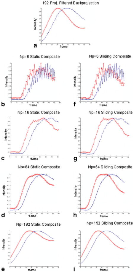
Signal vs. time curves derived from the arterial signal (solid circle) and the venous signal (dotted circle) are presented in Fig. 4. Curves for static and sliding composites are presented separately to compare the effects of using the two different composites. Note that images reconstructed with as few as six projections (Fig. 4c and h) have severe fluctuations in signal, and the time course cannot be determined. As more projections are used to reconstruct the images, the fidelity of the time course is improved but blurred, and the frame-to-frame fluctuations are reduced (Fig. 4g and l).
FIG. 4.
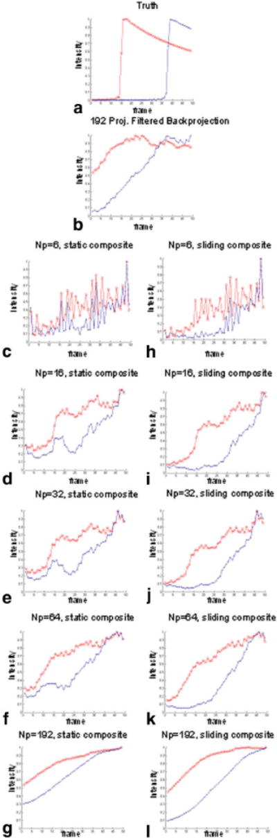
Signal curves for different image reconstructions base simulations. a: Truth. b: Filtered BP with NP = 192. c–g: Static composite (NP = 6, 16, 32, 64, 192). h–l: Sliding composite (NP = 6, 16, 32, 64, 192). [Color figure can be viewed in the online issue, which is available at www.interscience.wiley.com.]
The mean and SD of the image error as a function of the number of projections are reported in Table 1. In both sliding and static composites, using very few (six) or many (192) projections results in a higher image error. The image error is at the minimum when 16 projections are used with a static composite or when 32 projections are used with a sliding composite. The SD of image error, which shows the fluctuations of image error from one frame to the next, is at the minimum when 32 projections are used with a sliding composite or when 64 projections are used with a static composite. Overall, a 32-projection image with a sliding composite results in the lowest average image error and SD. The paired Student's t-test showed that the sliding composite results in significantly (P < 0.05) lower image error than the static composite.
The average SNR measured over time on an ROI drawn on the top bolus model showed an increasing trend as more projections were used. The SNR values for static composite images were greater than those of the sliding composite images of the corresponding number of projections.
AVM Patient Studies
The patient study showed results similar to those observed in simulations. Figure 5 shows representative sagittal projections of an angiographically confirmed AVM (Fig. 5d). Images were reconstructed using a sliding composite with NP = 6, 32, and 192 projections for Fig. 5a–c, respectively. These images demonstrate the trade-off between the numbers of projections used in the reconstruction. As more projections are used, the temporal footprint becomes broader, resulting in undesired artifactual increase in signal intensity in the superior sagittal sinus prior to the arrival of contrast agent. Using fewer projections shows an increase in streak artifacts as shown in Fig. 5a.
FIG. 5.
AVM patient images reconstructed with a sliding composite image: (a) NP = 6 sliding composite HYPR, (b) NP = 32 sliding composite HYPR, (c) NP = 192 sliding composite HYPR, and (d) X-ray angiogram. Dotted arrows indicate radial streak artifacts with a small NP. Solid arrows indicate varying degree of early venous phase due to different numbers of projections.
Figure 6 shows the corresponding arterial and venous signal vs. time curves. Images that were reconstructed using a small number of projections (NP = 6 in Fig. 6b, NP = 16 in Fig. 6c) resulted in temporal profiles with large frame-to-frame fluctuations. As more projections were added, the profiles became smoother, but the plots showed temporal blurring, characterized by a broader profile indicating early and prolonged contrast enhancement.
FIG. 6.
Temporal profile of ROIs (artery: red; vein: blue) of an AVM: (a) filtered BP, (b–e) static composite (Np = 6,16, 64,192), and (f–i) sliding composite (Np = 6, 16, 64, 192).
The results comparing SNR, CNR, and overlap integral are shown in Table 2. The results of the regular filtered BP are shown to provide a reference. There are several trends in the table. In almost all cases, the mean SNR and mean CNR values are higher in HYPR-processed images with the static composite than with the sliding composite. The overlap integral is also highest for static composite images. These data also demonstrate a trend of increasing SNR as the number of projections is increased. The highest mean CNR values were seen for NP values between 16 and 64. Note that in some extreme cases with static composite HYPR using 192 projections, the CNR values resulted in zero, meaning that the artery and vein were enhanced simultaneously. The trend of increasing overlap integral as number of projections is increased is observed in both sliding and static composites. HYPR images with NP between 16 and 64 showed improvement in CNR, SNR, and overlap integral values over filtered BP without HYPR.
Table 2.
Table of Maximum CNR, Maximum SNR, and Overlap Integral (OI) of AVM Patients*
| NP | Mean CNR | Mean SNR | Overlap integral | |||
|---|---|---|---|---|---|---|
| Static composite | Sliding composite | Static composite | Sliding composite | Static composite | Sliding composite | |
| Patient 1 | ||||||
| 4 | 29.25 | 49.17 | 29.48 | 51.01 | 18.00 | 20.26 |
| 16 | 42.29 | 67.93 | 43.23 | 71.63 | 22.84 | 25.17 |
| 32 | 47.49 | 68.87 | 48.31 | 76.22 | 24.34 | 26.98 |
| 64 | 53.73 | 73.22 | 55.15 | 79.86 | 27.33 | 30.66 |
| 128 | 53.00 | 62.66 | 60.62 | 83.26 | 34.27 | 38.90 |
| No HYPR | 42.98 | 43.83 | 31.54 | |||
| Patient 2 | ||||||
| 4 | 22.71 | 179.50 | 39.74 | 217.13 | 20.48 | 25.11 |
| 16 | 33.22 | 233.97 | 57.24 | 284.96 | 26.40 | 32.79 |
| 32 | 39.71 | 252.51 | 65.10 | 307.69 | 28.20 | 35.12 |
| 64 | 43.83 | 257.20 | 73.31 | 317.97 | 31.95 | 40.01 |
| 128 | 33.18 | 225.80 | 78.28 | 293.71 | 42.83 | 53.66 |
| No HYPR | 24.20 | 63.68 | 39.68 | |||
| Patient 3 | ||||||
| 6 | 7.24 | 13.24 | 31.31 | 40.39 | 32.09 | 33.96 |
| 16 | 7.23 | 14.38 | 34.34 | 52.16 | 50.90 | 59.13 |
| 32 | 7.54 | 51.03 | 41.09 | 147.06 | 38.80 | 41.69 |
| 64 | 8.49 | 30.56 | 48.21 | 150.81 | 40.15 | 43.86 |
| 192 | 7.15 | 0.00 | 58.99 | 151.08 | 48.26 | 54.59 |
| No HYPR | 11.37 | 47.82 | 44.28 | |||
| Patient 4 | ||||||
| 6 | 23.72 | 41.63 | 39.04 | 79.11 | 34.32 | 41.86 |
| 16 | 30.17 | 48.04 | 47.53 | 89.37 | 39.21 | 48.82 |
| 32 | 35.46 | 49.51 | 52.99 | 91.95 | 39.97 | 50.24 |
| 64 | 41.41 | 46.76 | 59.98 | 91.14 | 41.24 | 52.32 |
| 192 | 10.77 | 31.36 | 67.81 | 78.25 | 43.84 | 64.17 |
| No HYPR | 7.45 | 49.08 | 38.42 | |||
| Patient 5 | ||||||
| 6 | 15.51 | 19.32 | 27.65 | 33.51 | 34.27 | 40.19 |
| 16 | 18.56 | 22.31 | 36.91 | 46.44 | 36.53 | 42.78 |
| 32 | 21.04 | 21.65 | 43.04 | 51.52 | 36.62 | 43.03 |
| 64 | 23.29 | 19.88 | 48.55 | 56.68 | 36.26 | 42.65 |
| 192 | 7.64 | 0.00 | 59.57 | 63.21 | 34.15 | 38.63 |
| No HYPR | 13.26 | 33.96 | 38.92 | |||
Table of mean CNR, mean SNR, and overlap integral (OI) of AVM patient images reconstructed with HYPR using sliding or static composites with varying number of projections (NP = 6-192) and 192-projection filtered backprojection (no HYPR).
Figure 7 shows the plot of qualitative scores of image quality evaluated blindly by a radiologist. For the sliding composite HYPR, the dynamic information is best for the six-projection images, and the score decreases as more projections are used. For the static composite, however, using small number of projections actually lowers the dynamic information score. The worst dynamic information was recorded for 192-projection HYPR with the static composite. The SNR/artifact scores are the lowest for six-projection HYPR images. The scores are better for images with the number of projections greater than 6, but in general do not depend on the composite type or number of projections. The scores of the best HYPR images were for NP between 16 and 64. While SNR/artifact scores were similar for sliding and static composites for NP = 16–64, the sliding composite scored better on dynamic information. The scores for visualization of feeders, nidus, and draining veins did not vary significantly for the different number of projections or the composite types, or for regular filtered BP with sliding window.
FIG. 7.
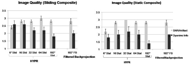
Image quality was scored by a radiologist in two categories qualitatively: dynamic information and SNR/artifact levels. “Slid.” and “Stat.” indicate sliding and static composites, respectively. *In two cases, 128 projections were acquired in each repetition, and NP = 4 and 128 was used instead of NP = 6 and 192.
Discussion
We have found that by using HYPR with a sliding composite, SNR is increased without significant changes in temporal profile compared to standard filtered BP. A static composite yields even higher SNR but temporal information is blurred. Thus, the size of the window for the composite is a trade-off between temporal information and SNR. Using a smaller number of projections shows benefits of decreasing temporal blur, indicated by a smaller overlap integral, but at the same time it causes large projection-dependent fluctuations in temporal profiles, manifested by flashing of the dynamic series of the images. Using the full number of projections yields a very smooth profile, but the long temporal footprint results in temporal blurring, as shown in AVM patient plots. We found the optimal imaging parameter to be NP = 32 with a sliding composite, which resulted in the lowest image error while achieving higher SNR and CNR than filtered BP with acceptable temporal dynamics. Through radiologist readings, systematic improvement in SNR and dynamic information for HYPR images from conventional filtered BP images was seen for HYPR images with 16–64 projections with sliding composites, though the improvements were small.
Large fluctuations in the temporal profiles and image error from HYPR images reconstructed from fewer projections can be attributed to the different set of angles used for reconstruction of each frame. If one of the few projections used in reconstruction happens to be close to being perpendicular to the direction of the bolus, the reconstructed image of it will be a line of bolus that extends from one end to the other, which is not a good representation of the image. And since there are only a small number of projections, this projection has more weight in determining the reconstructed image than with a larger number of projections. Moreover, since angular ordering is scheduled so that there are periodically angles that are perpendicular or close to perpendicular to the path of the bolus, periodic spikes can be seen. As we increase the number of projections, the weight of the “bad projection” in determining the reconstructed image decreases, and the fluctuation amplitude decreases. Huang and Wright (29) previously showed in simulations the effects of HYPR processing in the temporal profiles of objects and cross-talk between multiple objects. However, the simulations were limited to stationary objects with intensities varying over time; in clinical situations, the bolus of contrast agent physically moves along the direction of the blood vessels.
SNR and CNR benefits of HYPR were observed in both simulations and AVM patient studies. In simulations, average SNR values over time were greater for all HYPR reconstructions than conventional filtered BP with 192 projections, which was expected since the static and sliding composites contain about 8 and 2.5 times more data, respectively, than filtered BP. It was also found that the SNR increased as more projections were used. In the AVM patient studies, we found that SNR and CNR increased in every case with the right choice of NP, which ranged between 16 and 64. The images with static composites have higher SNR than sliding composite HYPR and regular filtered BP images without any HYPR processing, because the static composite is signal averaged over several measurements with high signal. However, the static composite cannot maintain the temporal profile as well as the sliding composite, as shown by early venous enhancement and prolonged arterial enhancement in the patient images. If the composite includes information that is too far ahead in time, it introduces signals that should not appear in the current time frame. Figure 6 shows that arterial signals stay higher in static composites than sliding composites because the static composite's temporal footprint covers more of the past information than the sliding composite. The sliding composite reduces this effect by limiting the past temporal information included in the composite. Therefore, deciding what kind of composite to use is a trade-off between temporal information and SNR.
In some data sets, CNR was actually lowest when the highest number of projections is used. Temporal blurring that results from a large number of projections makes the bolus profile broader, decreasing the contrast between artery and vein, even though the SNR is higher due to less undersampling artifacts. Low CNR is also observed in some cases with the fewest projections. In this case, lower SNR from the streak artifacts from angular undersampling dominates over the sharper bolus profile from a small number of projections. Overall, the highest CNR occurs between 16 and 64 projection HYPR images.
In this work we analyzed the effects of HYPR on artifact and noise separately. While the number of projections controls fluctuations in signal and radial undersampling artifacts and temporal blur, the length of the composite controls the SNR as well as temporal blur. In our study, 32 was determined to be the minimum number of projections that results in an acceptable level of signal fluctuations and radial streak artifacts, which probably will not depend on other imaging parameters. However, the effects of the composite length can be simplified to SNR vs. acquisition time. It is a well-known fact that SNR is proportional to the square root of imaging time. Likewise, a longer composite, with more signal-averaged repetitions, yields images with higher SNR. This result agrees with previous studies (27– 29). Therefore, the optimal length of the composite will depend on other parameters that affect acquisition time, such as TR, Nθ, and NSlices. The difference between HYPR and a simple long-acquisition MRA with signal averaging is that the long temporal footprint of HYPR is weighted and distributed to limited projection images, recovering some temporal information while producing artifacts characterized by fluctuations and flashing of signals.
Aside from the quantitative conclusions from the data, the qualitative effects of HYPR, seen through the eyes of a clinician, seem less pronounced. The results from the radiologist's reading agree with the quantitative analysis on the trends observed with quantitative SNR and image error measurements: more projections improve SNR and artifact levels, and less projections result in better dynamic information. However, from the fact that the conventional filtered BP method with sliding window scored not too far below the best HYPR methods qualitatively, it is still questionable whether the SNR gains and better dynamic information from HYPR are significant enough to convince a radiologist of its diagnostic power, especially considering the processing overhead involved with HYPR.
This study had some limitations. True SNR calculations for HYPR images, which are still under debate, are rather complicated and involve knowledge of the number of vascular pixels, number of projections used, and number of frames, as well as the SNR of the composite (27,29,31). However, we were interested in how the HYPR images compare against non-HYPR-processed images using a metric that is not calculated differently for HYPR. Therefore, we used an operational definition of SNR, the average value inside the ROI divided by the SD of air, which still results in SNR values that can be used for comparison. Another limitation, which is intrinsic to the technique, is that there is still a broad temporal footprint. Even with limited projections, processing with HYPR adds the long temporal footprint of the composite. A possible remedy for this problem is using parallel imaging in either the radial (32) or through-plane direction (33) in the sequence to reduce the acquisition time required for one frame. Finally, the computational time of the HYPR algorithm is not trivial; reconstruction of a full time series with one NP value takes about 10 h to reconstruct using MATLAB on an average personal computer.
Conclusions
Effects of HYPR processing with static and sliding composites on MRA images were studied in simulations and patients with intracranial AVMs. From the quantitative analysis, it was determined that the static composite boosts the SNR of standard filtered BP images, but temporal information is lost. The sliding composite, which has a smaller window of averaged frames, yields images with lower SNR than the static composite, but the sliding composite maintains temporal information better than the static composite. We have also shown that a smaller number of projections resulted in fluctuations in signal and image error. As the number of projections increased, fluctuations were reduced, but signal was blurred in time. However, in the radiologist's readings, improvements made by HYPR were more subtle. The optimal parameter that improves SNR while maintaining the temporal dynamics compared to standard filtered BP was determined to be NP = 32 with a sliding composite.
Acknowledgments
This work was supported by National Institutes of Health (NHLBI) R01 088437.
References
- 1.Prince MR, Yucel EK, Kaufman JA, Harrison DC, Geller SC. Dynamic gadolinium-enhanced three-dimensional abdominal MR arteriography. J Magn Reson Imaging. 1993;3:877–881. doi: 10.1002/jmri.1880030614. [DOI] [PubMed] [Google Scholar]
- 2.Riederer SJ, Tasciyan T, Farzaneh F, Lee JN, Wright RC, Herfkens RJ. MR fluoroscopy: technical feasibility. Magn Reson Med. 1988;8:1–15. doi: 10.1002/mrm.1910080102. [DOI] [PubMed] [Google Scholar]
- 3.Wang Y, Weber DM, Korosec FR, Mistretta CA, Grist TM, Swan JS, Turski PA. Generalized matched filtering for time-resolved MR angiography of pulsatile flow. Magn Reson Med. 1993;30:600–608. doi: 10.1002/mrm.1910300511. [DOI] [PubMed] [Google Scholar]
- 4.Maki JH, Prince MR, Londy FJ, Chenevert TL. The effects of time varying intravascular signal intensity and k-space acquisition order on three-dimensional MR angiography image quality. J Magn Reson Imaging. 1996;6:642–651. doi: 10.1002/jmri.1880060413. [DOI] [PubMed] [Google Scholar]
- 5.Earls JP, Rofsky NM, DeCorato DR, Krinsky GA, Weinreb JC. Breath-hold single-dose gadolinium-enhanced three-dimensional MR aortography: usefulness of a timing examination and MR power injector. Radiology. 1996;201:705–710. doi: 10.1148/radiology.201.3.8939219. [DOI] [PubMed] [Google Scholar]
- 6.Foo TK, Saranathan M, Prince MR, Chenevert TL. Automated detection of bolus arrival and initiation of data acquisition in fast, three-dimensional, gadolinium-enhanced MR angiography. Radiology. 1997;203:275–280. doi: 10.1148/radiology.203.1.9122407. [DOI] [PubMed] [Google Scholar]
- 7.Wilman AH, Riederer SJ, King BF, Debbins JP, Rossman PJ, Ehman RL. Fluoroscopically triggered contrast-enhanced three-dimensional MR angiography with elliptical centric view order: application to the renal arteries. Radiology. 1997;205:137–146. doi: 10.1148/radiology.205.1.9314975. [DOI] [PubMed] [Google Scholar]
- 8.Ho KY, Leiner T, de Haan MW, Kessels AG, Kitslaar PJ, van Engelshoven JM. Peripheral vascular tree stenoses: evaluation with moving-bed infusion-tracking MR angiography. Radiology. 1998;206:683–692. doi: 10.1148/radiology.206.3.9494486. [DOI] [PubMed] [Google Scholar]
- 9.Hany TF, Leung DA, Pfammatter T, Debatin JF. Contrast-enhanced magnetic resonance angiography of the renal arteries. Original investigation. Invest Radiol. 1998;33:653–659. doi: 10.1097/00004424-199809000-00021. [DOI] [PubMed] [Google Scholar]
- 10.Meaney JF, Ridgway JP, Chakraverty S, Robertson I, Kessel D, Radjenovic A, Kouwenhoven M, Kassner A, Smith MA. Stepping-table gadolinium-enhanced digital subtraction MR angiography of the aorta and lower extremity arteries: preliminary experience. Radiology. 1999;211:59–67. doi: 10.1148/radiology.211.1.r99ap1859. [DOI] [PubMed] [Google Scholar]
- 11.Korosec FR, Turski PA, Carroll TJ, Mistretta CA, Grist TM. Contrast-enhanced MR angiography of the carotid bifurcation. J Magn Reson Imaging. 1999;10:317–325. doi: 10.1002/(sici)1522-2586(199909)10:3<317::aid-jmri14>3.0.co;2-m. [DOI] [PubMed] [Google Scholar]
- 12.Kruger DG, Riederer SJ, Grimm RC, Rossman PJ. Continuously moving table data acquisition method for long FOV contrast-enhanced MRA and whole-body MRI. Magn Reson Med. 2002;47:224–231. doi: 10.1002/mrm.10061. [DOI] [PubMed] [Google Scholar]
- 13.Finn JP, Baskaran V, Carr JC, McCarthy RM, Pereles FS, Kroeker R, Laub GA. Thorax: low-dose contrast-enhanced three-dimensional MR angiography with subsecond temporal resolution—initial results. Radiology. 2002;224:896–904. doi: 10.1148/radiol.2243010984. [DOI] [PubMed] [Google Scholar]
- 14.Carr JC, Nemcek AA, Jr, Abecassis M, Blei A, Clarke L, Pereles FS, McCarthy R, Finn JP. Preoperative evaluation of the entire hepatic vasculature in living liver donors with use of contrast-enhanced MR angiography and true fast imaging with steady-state precession. J Vasc Interv Radiol. 2003;14:441–449. doi: 10.1097/01.rvi.0000064853.87207.42. [DOI] [PubMed] [Google Scholar]
- 15.Greenberg MS. Handbook of neurosurgery. New York: Thieme Medical Publishers; 2001. p. 971 p. [Google Scholar]
- 16.Spetzler RF, Martin NA. A proposed grading system for arteriovenous malformations. J Neurosurg. 1986;65:476–483. doi: 10.3171/jns.1986.65.4.0476. [DOI] [PubMed] [Google Scholar]
- 17.Spetzler RF, Martin NA, Carter LP, Flom RA, Raudzens PA, Wilkinson E. Surgical management of large AVM's by staged embolization and operative excision. J Neurosurg. 1987;67:17–28. doi: 10.3171/jns.1987.67.1.0017. [DOI] [PubMed] [Google Scholar]
- 18.Goldfarb JW, Prasad PV, Griswold MA, Edelman RR. Dynamic three-dimensional magnetic resonance abdominal angiography and perfusion: implementation and preliminary experience. J Magn Reson Imaging. 2000;11:201–207. doi: 10.1002/(sici)1522-2586(200002)11:2<201::aid-jmri19>3.0.co;2-4. [DOI] [PubMed] [Google Scholar]
- 19.Sodickson DK, Manning WJ. Simultaneous acquisition of spatial harmonics (SMASH): fast imaging with radiofrequency coil arrays. Magn Reson Med. 1997;38:591–603. doi: 10.1002/mrm.1910380414. [DOI] [PubMed] [Google Scholar]
- 20.Pruessmann KP, Weiger M, Scheidegger MB, Boesiger P. SENSE: sensitivity encoding for fast MRI. Magn Reson Med. 1999;42:952–962. [PubMed] [Google Scholar]
- 21.Sodickson DK, McKenzie CA, Li W, Wolff S, Manning WJ, Edelman RR. Contrast-enhanced 3D MR angiography with simultaneous acquisition of spatial harmonics: a pilot study. Radiology. 2000;217:284–289. doi: 10.1148/radiology.217.1.r00se47284. [DOI] [PubMed] [Google Scholar]
- 22.Weiger M, Pruessmann KP, Kassner A, Roditi G, Lawton T, Reid A, Boesiger P. Contrast-enhanced 3D MRA using SENSE. J Magn Reson Imaging. 2000;12:671–677. doi: 10.1002/1522-2586(200011)12:5<671::aid-jmri3>3.0.co;2-f. [DOI] [PubMed] [Google Scholar]
- 23.Griswold MA, Jakob PM, Heidemann RM, Nittka M, Jellus V, Wang J, Kiefer B, Haase A. Generalized autocalibrating partially parallel acquisitions (GRAPPA) Magn Reson Med. 2002;47:1202–1210. doi: 10.1002/mrm.10171. [DOI] [PubMed] [Google Scholar]
- 24.Cashen TA, Jeong H, Shah MK, Bhatt HM, Shin W, Carr JC, Walker MT, Batjer HH, Carroll TJ. 4D radial contrast-enhanced MR angiography with sliding subtraction. Magn Reson Med. 2007;58:962–972. doi: 10.1002/mrm.21364. [DOI] [PMC free article] [PubMed] [Google Scholar]
- 25.Scheffler K, Hennig J. Reduced circular field-of-view imaging. Magn Reson Med. 1998;40:474–480. doi: 10.1002/mrm.1910400319. [DOI] [PubMed] [Google Scholar]
- 26.Peters DC, Korosec FR, Grist TM, Block WF, Holden JE, Vigen KK, Mistretta CA. Undersampled projection reconstruction applied to MR angiography. Magn Reson Med. 2000;43:91–101. doi: 10.1002/(sici)1522-2594(200001)43:1<91::aid-mrm11>3.0.co;2-4. [DOI] [PubMed] [Google Scholar]
- 27.Mistretta CA, Wieben O, Velikina J, Block W, Perry J, Wu Y, Johnson K. Highly constrained backprojection for time-resolved MRI. Magn Reson Med. 2006;55:30–40. doi: 10.1002/mrm.20772. [DOI] [PMC free article] [PubMed] [Google Scholar]
- 28.Wu Y, Kim N, Korosec FR, Turk A, Rowley HA, Wieben O, Mistretta CA, Turski PA. 3D time-resolved contrast-enhanced cerebrovascular MR angiography with subsecond frame update times using radial k-space trajectories and highly constrained projection reconstruction. AJNR Am J Neuroradiol. 2007;28:2001–2004. doi: 10.3174/ajnr.A0772. [DOI] [PMC free article] [PubMed] [Google Scholar]
- 29.Huang Y, Wright GA. Time-resolved MR angiography with limited projections. Magn Reson Med. 2007;58:316–325. doi: 10.1002/mrm.21312. [DOI] [PubMed] [Google Scholar]
- 30.Peters DC, Rohatgi P, Botnar RM, Yeon SB, Kissinger KV, Manning WJ. Characterizing radial undersampling artifacts for cardiac applications. Magn Reson Med. 2006;55:396–403. doi: 10.1002/mrm.20782. [DOI] [PubMed] [Google Scholar]
- 31.Griswold MA, Barkauskas K, Blaimer M, Sunshine JL, Duerk JL. More optimal HYPR reconstructions using a combination of HYPR and conjugate-gradient minimization. Proceedings of the 15th Annual Meeting of ISMRM; Berlin, Germany. 2007. Abstract 834. [Google Scholar]
- 32.Heidemann RM, Griswold MA, Jakob PM. Fast parallel image reconstruction for non-Cartesian trajectories. Proceedings of the 11th Annual Meeting of ISMRM; Toronto, Canada. 2003. Abstract 2347. [Google Scholar]
- 33.Cashen TA, Carroll TJ. Hybird radial-parallel 3D imaging. Proceedings of the 13th Annual Meeting of ISMRM; Miami Beach, FL, USA. 2005. Abstract 13. [Google Scholar]