A Robust Gene Selection Method for Microarray-based Cancer Classification

Abstract

Gene selection is of vital importance in molecular classification of cancer using high-dimensional gene expression data. Because of the distinct characteristics inherent to specific cancerous gene expression profiles, developing flexible and robust feature selection methods is extremely crucial. We investigated the properties of one feature selection approach proposed in our previous work, which was the generalization of the feature selection method based on the depended degree of attribute in rough sets. We compared the feature selection method with the established methods: the depended degree, chi-square, information gain, Relief-F and symmetric uncertainty, and analyzed its properties through a series of classification experiments. The results revealed that our method was superior to the canonical depended degree of attribute based method in robustness and applicability. Moreover, the method was comparable to the other four commonly used methods. More importantly, the method can exhibit the inherent classification difficulty with respect to different gene expression datasets, indicating the inherent biology of specific cancers.

Background

One major problem in applying gene expression profiles to cancer classification and prediction is that the number of features (genes) greatly surpasses the number of samples. Some studies have shown that a small collection of genes selected correctly can lead to good classification results.^1–4 Therefore gene selection is crucial in molecular classification of cancer. Numerous methods of selecting informative gene groups to conduct cancer classification have been proposed. Most of the methods first ranked the genes based on certain criteria, and then selected a small set of informative genes for classification from the top-ranked genes. The most used gene ranking approaches include t-score, chi-square, information entropy-based, Relief-F, symmetric uncertainty etc.

In,² we used a new feature selection method for gene selection. The feature selection method was based on the α depended degree, a generalized concept of the canonical depended degree proposed in rough sets. Combining this feature selection method with decision rules-based classifiers, we achieved accurate molecular classification of cancer by a small size of genes. As pointed out in,² our classification methods had some advantages over other methods in such as simplicity and interpretability. Yet, there remain some essential problems to be investigated. For example, what properties does the feature selection method possess, and what will happen if we compare the feature selection method with other feature selection methods in terms of identical classifiers?

In this work, we investigated the properties of the feature selection method based on the α depended degree. We mainly studied the relationships between α value, classifier, classification accuracy and gene number. Moreover, we compared our feature selection method with other four feature selection methods often used in practice: chi-square, information gain, Relief-F and symmetric uncertainty. We chose four popular classifiers: NB (Naive Bayes), DT (Decision Tree), SVM (Support Vector Machine) and k-NN (k-nearest neighbor), to carry out classification via the genes selected based on the different feature selection methods. Our study materials included the eight publicly available gene expression datasets: Colon Tumor, CNS (Central Nervous System) Tumor, DLBCL (Diffuse Large B-Cell Lymphoma), Leukemia 1 (ALL [Acute Lymphoblastic Leukemia] vs. AML [Acute Myeloid Leukemia]), Lung Cancer, Prostate Cancer, Breast Cancer, and Leukemia 2 (ALL vs. MLL [Mixed-Lineage Leukemia] vs. AML), which were downloaded from the Kent Ridge Bio-medical Data Set Repository (http://datam.i2r.a-star.edu.sg/datasets/krbd/).

Materials

Colon tumor dataset

The dataset contains 62 samples collected from Colon Tumor patients.⁵ Among them, 40 tumor biopsies are from tumors (labeled as “negative”) and 22 normal (labeled as “positive”) biopsies are from healthy parts of the colons of the same patients. Each sample is described by 2000 genes.

CNS tumor dataset

The dataset is about patient outcome prediction for central nervous system embryonal tumor.⁶ In this dataset, there are 60 observations, each of which is described by the gene expression levels of 7129 genes and a class attribute with two distinct labels—Class 1 (survivors) versus Class 0 (failures). Survivors are patients who are alive after treatment while the failures are those who succumbed to their disease. Among 60 patient samples, 21 are labeled as “Class 1” and 39 are labeled as “Class 0”.

DLBCL dataset

The dataset is about patient outcome prediction for DLBCL.⁷ The total of 58 DLBCL samples are from 32 cured patients (labeled as “cured”) and 26 refractory patients (labeled as “fatal”). The gene expression profile contains 7129 genes.

Leukemia 1 dataset (ALL vs. AML)

In this dataset,¹ there are 72 observations, each of which is described by the gene expression levels of 7129 genes and a class attribute with two distinct labels—AML versus ALL.

Lung cancer dataset

The dataset is on classification of MPM (Malignant Pleural Mesothelioma) versus ADCA (Adenocarcinoma) of the lung.⁸ It is composed of 181 tissue samples (31 MPM, 150 ADCA). Each sample is described by 12533 genes.

Prostate cancer dataset

The dataset is involved in prostate tumor versus normal classification. It contains 52 prostate tumor samples and 50 non-tumor prostate samples.⁹ The total number of genes is 12600. Two classes are denoted as “Tumor” and “Normal”, respectively.

Breast cancer dataset

The dataset is about patient outcome prediction for breast cancer.¹⁰ It contains 78 patient samples, 34 of which are from patients who had developed distant metastases within 5 years (labeled as “relapse”), the rest 44 samples are from patients who remained healthy from the disease after their initial diagnosis for interval of at least 5 years (labeled as “non-relapse”). The number of genes is 24481.

Leukemia 2 dataset (ALL vs. MLL vs. AML)

The dataset is about subtype prediction for leukemia.¹¹ It contains 57 samples (20 ALL, 17 MLL and 20 AML). The number of genes is 12582.

Methods

α Depended degree-based feature selection approach

In reality, when we are faced with a collection of new data, we often want to learn about them based on pre-existing knowledge. However, most of these data cannot be precisely defined based on pre-existing knowledge, as they incorporate both definite and indefinite components. In rough sets, one knowledge is formally defined as an equivalence relation. Accordingly, the definite components are represented with the concept of positive region.

Definition 1 Let U be a universe of discourse, X ⊆ U, and R is an equivalence relation on U. U/R represents the set of the equivalence class of U induced by R. The positive region of X on R is defined as pos(R, X) = ∪ {Y ∈ U/R | Y ⊆ X}.¹²

The decision table is the data form studied by rough sets. One decision table can be represented as S = (U, A = C ∪ D), where U is the set of samples, C is the condition attribute set, and D is the decision attribute set. Without loss of generality, hereafter we assume D is a single-element set, and we call D the decision attribute. In the decision table, the equivalence relation R(A’) induced by the attribute subset A’ ⊆ A is defined as: for ∀x, y ∈ U, xR(A’)y, if and only if I_a(x) = I_a(y) for each a ∈ A’, where I_a is the function mapping a member (sample) of U to the value of the member on the attribute a.

For the cancer classification problem, every collected set of microarray data can be represented as a decision table in the form of Table 2. In the microarray data decision table, there are m samples and n genes. Every sample is assigned to one class label. The expression level of gene y in sample x is represented by g(x, y).

Table 2.

Microarray data decision table.

Samples	Condition attributes (genes)				Decision attributes (classes)
	Gene 1	Gene 2	…	Genen	Class label
1	g(1, 1)	g(1, 2)	…	g(1, n)	Class (1)
2	g(2, 1)	g(2, 2)	…	g(2, n)	Class (2)
…	…	…	…	…	…
…	…	…	…	…	…
m	g(m, 1)	g(m, 2)	…	g(m, n)	Class (m)

In rough sets, the depended degree of a condition attribute subset P by the decision attribute D is defined as

$${\gamma }_P(D)=\frac{|{\text{POS}}_P(D)|}{\left|U\right|},$$

where $|{\mathit{\text{POS}}}_P(D)|=|\underset{X\in U/R(D)}{\cup }\mathit{\text{pos}}(P,\hspace{0.17em}X)|$ represents the size of the union of the positive region of each equivalence class in U/R(D) on P in U, and |U| represents the size of U (set of samples).

In some sense, γ_P(D) reflects the class-discrimination power of P. The greater is γ_P(D), the stronger the classification ability P is inclined to possess. Therefore, the depended degree can be used as the basis of feature selection. Actually, it has been applied in microarraybased cancer classification by some authors.^13,14

However, the extremely strict definition has limited its applicability. Hence, in,² we defined the α depended degree, a generalization form of the depended degree, and utilized the α depended degree as the basis for choosing genes. The α depended degree of an attribute subset P by the decision attribute D was defined as ${\gamma }_P(D,\hspace{0.17em}\alpha )=\frac{|{\text{POS}}_P(D,\hspace{0.17em}\alpha )|}{\left|U\right|}$, where 0 ≤ α ≤ 1, $|{\text{POS}}_P(D,\hspace{0.17em}\alpha )|=|\underset{X\in U/R(D)}{\cup }\mathit{\text{pos}}(P,\hspace{0.17em}X,\hspace{0.17em}\alpha )|$ and pos(P, X, α) = ∪ {Y ∈ U/R(P)| |Y ∩ X|/|Y| ≥ α}. As a result, the depended degree became a specific case of the α depended degree when α = 1. For the selection of indeed high class-discrimination genes, we have set the lower limit of α value as 0.7 in practice.²

Comparative feature selection approaches

We compared our proposed feature selection method with the following four often used methods: chi-square, information gain, Relief-F and symmetric uncertainty.

The chi-square (χ²) method evaluates features individually by measuring their chi-squared statistic with respect to the classes.¹⁵ The χ² value of an attribute a is defined as follows:

$${\chi }^2(a)=\sum _{v\in V}\sum _{i=1}^n\frac{[A_i(a=v)-E_i{(a=v)]}^2}{E_i(a=v)},$$

where V is the set of possible values for a, n the number of classes, A_i(a = v) the number of samples in the ith class with a = v, and E_i(a = v) the expected value of A_i(a = v); E_i(a = v) = P(a = v)P(c_i)N, where P(a = v) is the probability of a = v, P(c_i) the probability of one sample labeled with the ith class, and N the total number of samples.

Information Gain¹⁶ method selects the attribute with highest information gain, which measures the difference between the prior uncertainty and expected posterior uncertainty caused by attributes. The information gain by branching on an attribute a is defined as:

$$\mathit{\text{Info}}\_\mathit{\text{Gain}}(S,\hspace{0.17em}a)=E(S)-\sum _{i=1}^n\frac{S_i}{S}E(S_i),$$

where E(S) is the entropy before split, $\sum _{i=1}^n\frac{S_i}{S}E(S_i)$ the weighted entropy after split, and {S₁, S₂, …, S_n} the partition of sample set S by a values.

Relief-F method estimates the quality of features according to how well their values distinguish between examples that are near to each other. Specifically, it tries to find a good estimate of the following probability to assign as the weight for each feature a:¹⁷ w_a = P (different value of a | different class) – P(different value of a | same class). Differing from the majority of the heuristic measures for estimating the quality of the attributes assume the conditional independence of the attributes and are therefore less appropriate in problems which possibly involve much feature interaction. Relief algorithms (including Relief-F) do not make this assumption and therefore are efficient in estimating the quality of attributes in problems with strong dependencies between attributes.¹⁸

Symmetric uncertainty method compensates for information gain’s bias towards features with more values. It is defined as:

$$SU(X,\hspace{0.17em}Y)=2\frac{IG(X|Y)}{H(X)+H(Y)},$$

where H(X) and H(Y) are the entropy of attribute X and Y respectively, and IG(X|Y) = H(X) – H(X|Y) (H(X|Y) is the conditional entropy of X given Y), represents additional information about X provided by attribute Y. The entropy and conditional entropy are respectively defined as:

$$\begin{array}{c}H(X)=-\sum _{i}P(x_i){\text{log}}_2(P(x_i)),\\ H(X|Y)=-\sum _{j}P(y_j)\sum _{i}P(x_i|y_j){\text{log}}_2(P(x_i|y_j)).\end{array}$$

The values of symmetric uncertainty lie between 0 and 1. A value of 1 indicates that knowing the values of either attribute completely predicts the values of the other; a value of 0 indicates that X and Y are independent.

Classification algorithms

The NB classifier is a probabilistic algorithm based on Bayes’ rule and the simple assumption that the feature values are conditionally independent given the class. Given a new sample observation, the classifier assigns it to the class with the maximum conditional probability estimate.

DT is the rule-based classifier with non-leaf nodes representing selected attributes and leaf nodes showing classification outcomes. Every path from the root to a leaf node reflects a classification rule. We use the J4.8 algorithm, which is the Java implementation of C4.5 Revision 8.

An SVM views input data as two sets of vectors in an n-dimensional space, and constructs a separating hyperplane in that space, one which maximizes the margin between the two data sets. The SVM used in our experiments utilizes an SMO (Sequential Minimal Optimization) algorithm with polynomial kernels for training.

k-NN is an instance-based classifier. The classifier decides the class label of a new testing sample by the majority class of its k closest neighbors based on their Euclidean distance. In our experiments, k is set as 5.

Data preprocess

Because chi-square, information gain, symmetric uncertainty and our feature selection methods are suitable for discrete attribute values, we need to carry out the discretization of attribute values before feature selection using these methods. We used the entropy-based discretization method, which was proposed by Fayyad et al.¹⁹ This algorithm recursively applies an entropy minimization heuristic to discretize the continuous-valued attributes. The stop of the recursive step for this algorithm depends on the MDL (Minimum Description Length) principle.

Feature selection and classification

We ranked the genes in a descendent order of their α depended degree, and then used the top 100, 50, 20, 10, 5, 2 and 1 genes for classification with the four classifiers, respectively. In addition, we observed the classification results with the seven different α values: 1, 0.95, 0.9, 0.85, 0.8, 0.75 and 0.7. Moreover, we used the top 100, 50, 20, 10, 5, 2 and 1 genes ranked by the other four feature selection methods for classification with the four classifiers, respectively. Considering that the sample size in every dataset was relatively small, we used LOOCV (Leave-One-Out Cross-Validation) method to test the classification accuracy.

We implemented the data preprocess, feature selection and classification algorithms mainly in the Weka package.²⁰

Results and Analysis

Classification results using our feature selection method

Table 3 shows the classification results based on the α depended degree in the Colon Tumor dataset. The classification results in the other datasets based on the α depended degree were provided in the supplementary materials (1).

Table 3.

Classification accuracy (%) in the Colon tumor dataset based on the α depended degree.

α	Gene number	NB	DT	SVM	k-NN
1	100	74.19	88.71	87.10	88.71
	50	77.42	74.19	83.87	85.48
	20	79.03	83.87	88.71	85.48
	10	80.65	79.03	82.26	82.26
	5	75.81	61.29	59.68	67.74
	2	74.19	70.97	64.52	79.03
	1	74.19	70.97	64.52	72.58
0.95	100	75.81	88.71	83.87	83.87
	50	77.42	80.65	83.87	82.26
	20	80.65	77.42	72.58	72.58
	10	74.19	75.81	67.74	69.35
	5	72.58	75.81	56.45	75.81
	2	74.19	75.81	64.52	72.58
	1	74.19	77.42	64.52	67.74
0.90	100	77.42	88.71	85.48	87.10
	50	75.81	80.65	85.48	85.48
	20	80.65	74.19	85.48	87.10
	10	82.26	77.41	88.71	88.71
	5	72.58	85.48	79.03	88.71
	2	85.48	91.93	85.48	88.71
	1	75.81	82.26	72.58	77.42
0.85	100	79.03	87.10	87.10	85.48
	50	79.03	80.65	85.48	83.87
	20	80.65	80.65	87.10	87.10
	10	88.71	85.48	87.10	87.10
	5	87.10	87.10	85.48	88.71
	2	85.48	79.03	80.65	82.26
	1	85.48	85.48	77.42	85.48
0.80	100	80.65	87.10	87.10	85.48
	50	83.87	87.10	85.48	85.48
	20	85.48	80.65	87.10	88.71
	10	85.48	83.87	82.26	87.10
	5	83.87	80.65	82.26	82.26
	2	82.26	85.48	82.26	82.26
	1	83.87	82.26	75.81	80.65
0.75	100	79.03	87.10	85.48	85.48
	50	85.48	87.10	85.48	85.48
	20	87.10	82.26	83.87	85.48
	10	85.48	79.03	82.26	82.26
	5	85.48	85.48	82.26	82.26
	2	61.29	58.06	64.52	72.58
	1	67.74	67.74	64.52	72.58
0.70	100	82.26	87.10	85.48	85.48
	50	83.87	87.10	88.71	87.10
	20	87.10	90.32	87.10	85.48
	10	83.87	83.87	85.48	85.48
	5	83.87	69.35	83.87	85.48
	2	82.26	79.03	80.65	82.26
	1	67.74	67.74	64.52	72.58

The maximum numbers in each row are highlighted in boldface, indicating the highest classification accuracy achieved by among the different classifiers under the identical α value and gene number.

Comparison of classification performance for different classifiers

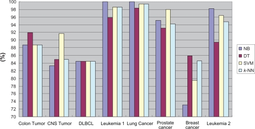
Table 3 shows that there are in total 12, 19, 11 and 20 best classification cases for NB, DT, SVM and k-NN, respectively. Table 4 shows the number of the best classification cases achieved by among the different classifiers under the identical α value and gene number for each dataset. Figure 1 presents the best classification accuracy of each classifier using our feature selection algorithm. From Table 4 and Figure 1, we noticed that combining our feature selection method with the NB classifier was inclined to achieve the best classification accuracy.

Table 4.

Number of best classification cases among the different classifiers.

Dataset/Classifier	NB	DT	SVM	k-NN
Colon tumor	12	19	11	20
CNS tumor	4	13	20	20
DLBCL	18	11	16	13
Leukemia 1	24	13	14	10
Lung cancer	19	5	17	11
Prostate cancer	9	9	25	16
Breast cancer	3	27	3	19
Leukemia 2	26	11	15	13

The maximum numbers in each row are highlighted in boldface.

Figure 1.

Best classification accuracy of each classifier.

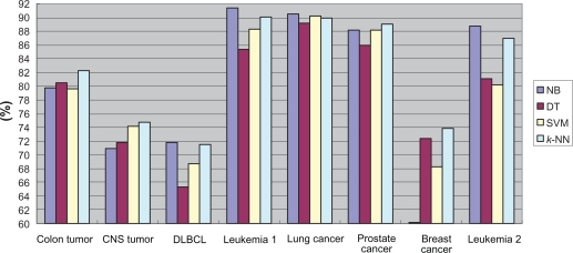
In addition, we considered the average classification performance. Table 5 shows the respective average classification accuracy of the four classifiers under different α values in the Colon Tumor dataset. The results revealed that the k-NN classifier had six best average classification performances under the seven α values, and it also had the best total average performance. Table 6 summarized the number of the best average classification performances achieved by each classifier under various α values for each dataset and the corresponding average number for each classifier within all of the eight datasets. Figure 2 lists the average classification accuracy of each classifier for each dataset, indicating that k-NN had the highest average accuracy in the Colon Tumor, CNS Tumor, Prostate Cancer and Breast Cancer datasets, while NB had the highest average accuracy in the other four datasets. Taken together, NB and k-NN possessed better classification performance with our feature selection approach than DT and SVM did. One possible explanation is that NB is the statistics-based classifier and k-NN is the instance-based classifier, while our feature selection method is concerned with both statistical and instantial factors.

Table 5.

Average classification accuracy (%) for the different classifiers and α values in the Colon tumor dataset.

α/Classifier	NB	DT	SVM	k-NN
1	76.50	75.58	75.81	80.18
0.95	75.58	78.80	70.51	74.88
0.9	78.57	82.95	83.18	86.18
0.85	83.64	83.64	84.33	85.71
0.80	83.64	83.87	83.18	84.56
0.75	78.80	78.11	78.34	80.87
0.7	81.57	80.64	82.26	83.41
Total average	79.76	80.51	79.66	82.26

The maximum numbers in each row are highlighted in boldface.

Table 6.

Number of the best average classification performances achieved by each classifier under various α values for each dataset.

Dataset/Classifier	NB	DT	SVM	k-NN
Colon tumor	0	1	0	6
Cns tumor	0	1	1	5
DLBCL	4	0	0	3
Leukemia 1	7	0	0	1
Lung cancer	4	0	3	0
Prostate cancer	1	0	2	4
Breast cancer	0	0	4	3
Leukemia 2	7	0	0	0
Total average	2.875	0.25	1.25	2.75

The maximum numbers in each row are highlighted in boldface.

Figure 2.

Average classification accuracy of each classifier.

The optimum gene size for classification depends on different classification algorithms. We found DT generally used fewer genes to reach the best accuracy compared with the other classification algorithms. This is one advantage of DT learning algorithm in that DT is a rule-based classifier and fewer genes will induce simpler classification rules, which in turn facilitate the interpretability of DT models.

Depended degree vs. α depended degree

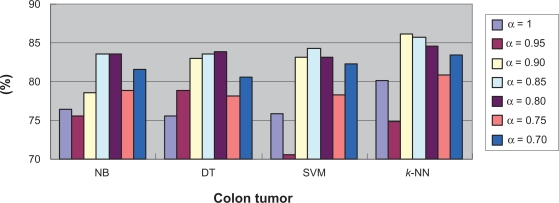
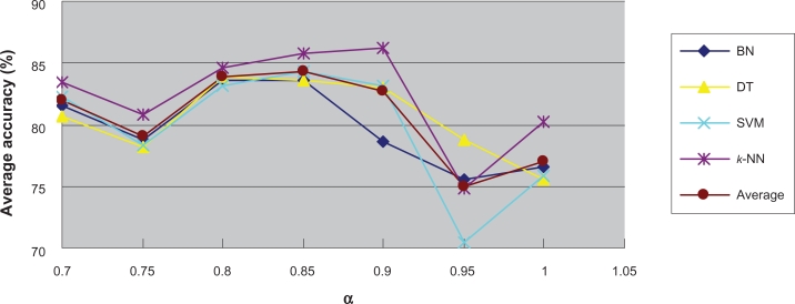
The depended degree was commonly applied in feature selection in rough sets-based machine learning and data mining. However, our recent studies have revealed that for the microarray-based cancer classification problem, the application of the depended degree was severely limited because of its overly rigor definition. In contrast, its generalized form-α depended degree, had essentially improved utility.² To explore how the classification quality was improved by using the α depended degree relative to the depended degree, we compared the classification results obtained under different α values while based on the identical classifiers. Figure 3 lists the average classification accuracies for different α values under the four different classifiers in the Colon Tumor dataset. The results shows that when NB was used for classification, the average classification accuracy in the case of the depended degree (α = 1) was only slightly better than the case of α = 0.95 and worse than all the other cases; when DT was used for classification, the average classification accuracy with the depended degree was the poorest; When SVM or k-NN was utilized as the classifier, the average classification performance in the case of the depended degree were both the second worst. When averaging the average classification accuracy of the four classifiers for each α value, we found that the result in the case of the depended degree was still the second worst. For the other datasets, the similar results were obtained. In fact, among the total of 32 average classification accuracy comparisons (4 classifiers × 8 datasets), the highest average classification accuracy was obtained with α = 1 only in three cases, wherein once shared by two different α values (see Fig. 3, and Fig. S1–7 in the supplementary materials (2)).

Figure 3.

Average classification accuracy for different α values.

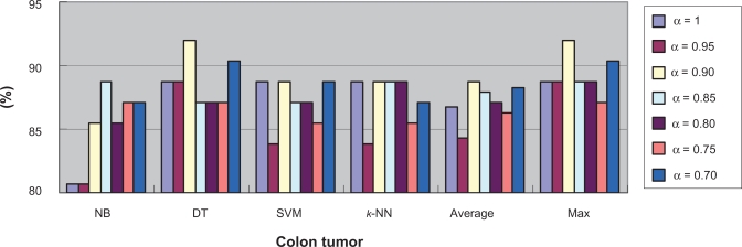
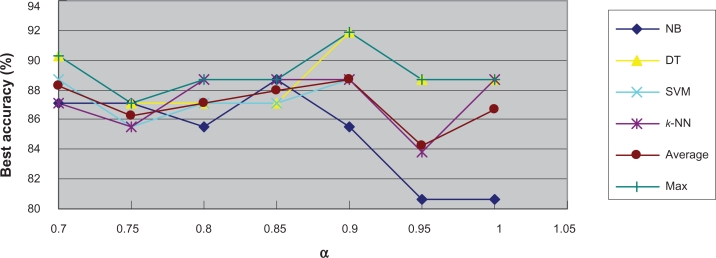
Further, we compared the best classification situations obtained under different α values. As shown in Table 7 and Figure 4, for the Colon Tumor dataset, in the cases of NB and DT, the best results were obtained when α = 0.85 and α = 0.9, respectively, although in the cases of SVM and k-NN, the best classification results were shared by several different α values including α = 1. When considering the average of the best classification accuracies for the four classifiers, as shown in the “Average” column, we found that the average best classification performance with α = 1 ranked fifth among the total of seven different α values; when considering the maximum of the best classification accuracies for the four classifiers, as shown in the “Max” column, we found that the maximum best classification performance with α = 1 was smaller than that with α = 0.9 or 0.7. The comparisons of the best classification results in the other datasets were provided in the supplementary materials (3).

Table 7.

Best classification accuracy (%) for the different classifiers and α values in the Colon tumor dataset.

α/Classifier	NB	DT	SVM	k-NN	Average	Max
1	80.65	88.71	88.71	88.71	86.70	88.71
0.95	80.65	88.71	83.87	83.87	84.28	88.71
0.9	85.48	91.93	88.71	88.71	88.71	91.93
0.85	88.71	87.1	87.1	88.71	87.91	88.71
0.80	85.48	87.1	87.1	88.71	87.10	88.71
0.75	87.1	87.1	85.48	85.48	86.29	87.1
0.7	87.1	90.32	88.71	87.1	88.31	90.32

The maximum numbers in each column are highlighted in boldface.

Figure 4.

Best classification accuracy for different α values.

All together, the α depended degree is a more effective feature selection method compared to the conventional depended degree.

Interrelation between classification accuracy and α value

In the previous studies,² we intuitively felt that the α value had some connections with inherent characters of related datasets. If the best classification accuracy was achieved only under relatively low α values, the dataset might be involved in relatively difficult classification and high classification accuracy would be hard to achieve. To prove this conjecture, we first detected the highest classification accuracies and their corresponding α values for each classifier, and calculated the averages of the accuracies and the averages of the α values under the four classifiers. For example, from Table 3, we knew that in the Colon Tumor dataset, NB had the highest accuracy of 88.71% accompanying with α = 0.85; DT had the highest accuracy of 91.93% accompanying with α = 0.9; SVM had the highest accuracy of 88.71% accompanying with α = 1, 0.9 and 0.7; k-NN had the highest accuracy of 88.71% accompanying with α = 1, 0.9 (occurring for three times), 0.85 and 0.8. We calculated the average of the accuracies as follows:

$$(88.71\%*3+91.93\%)/4=89.52\%;$$

and the average of the α values as follows:

$$\begin{array}{l}(0.85+0.9+(1+0.9+0.7)/3\\ +(1+0.9*3+0.85+0.8)/6)/4=\mathrm{0.8771.}\end{array}$$

We call this kind of average accuracies the average highest accuracy (AHA).

In addition, we calculated the average classification accuracy for each α-classifier pair, and found the best average accuracy and its corresponding α value for each classifier. Likewise, we calculated their averages under the four classifiers. For example, from Table 5, we knew that in the Colon Tumor dataset, α-NB had the best average accuracy of 83.64% with α = 0.8 and 0.85; α-DT had the best average accuracy of 83.87% with α = 0.8; α-SVM had the best average accuracy of 84.33% with α = 0.85; α-k-NN had the best average accuracy of 86.18% with α = 0.9. We calculated the average of the best average accuracies as follows:

$$(83.64\%+83.87\%+84.33\%+86.18\%)/4=89.52\%;$$

and the average of the α values as follows:

$$((0.8+0.85)/2+0.8+0.85+0.9)/4=\mathrm{0.8771.}$$

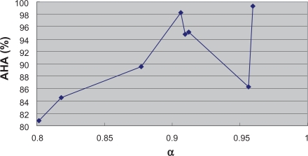
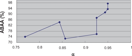
We call this kind of average accuracies the average best average accuracy (ABAA). The AHAs and ABAAs, and their corresponding α values in the other datasets were calculated in the same way. These results were presented in Table 8.

Table 8.

Average highest and best average classification accuracy (%).

Dataset	AHA (α)	ABAA (α)
Colon tumor	89.52 (0.8771)	84.51 (0.8438)
CNS tumor	86.25 (0.9563)	76.07 (0.925)
DLBCL	84.48 (0.8181)	72.91 (0.8563)
Leukemia 1	98.26 (0.9063)	93.80 (0.95)
Lung cancer	99.31 (0.9594)	97.61 (0.95)
Prostate cancer	95.11 (0.9125)	91.46 (0.9438)
Breast cancer	80.77 (0.8015)	74.08 (0.7688)
Leukemia 2	94.74 (0.9096)	87.47 (0.925)

The relatively bigger AHA, ABAA, α values and their corresponding datasets are highlighted in boldface, while the relatively smaller ones are highlighted in italic.

Figure 5 and Figure 6 reflect the alteration tendencies of AHA and ABAA along with the variation of α value, respectively. In general, AHA and ABAA increase with the growth of α value except for a few exceptions. Therefore, to a certain degree, the α depended degree can reflect the classification difficultness for a certain dataset, indicating the inherent biology of specific cancers. Indeed, the classification of Leukemia 1, Lung Cancer, Prostate Cancer and Leukemia 2 has been commonly recognized as relatively easy while the classification of Breast Cancer and DLBCL relatively difficult. Our results lend support to these findings.

Figure 5.

Relationship between AHA and α.

Figure 6.

Relationship between ABAA and α.

To further investigate the relationship between classification difficultness and α, we used the co-ordinates graph to show under different α values, the average and best classification results using every classifier. Figure 7 and Figure 8 show the results for the Colon Tumor dataset. From both figures, we inferred that in the dataset, the α values of between 0.8 and 0.9 would result to the best classification accuracy generally. We stated such α value the optimum α value. The optimum α values for the other datasets can be detected through the similar co-ordinates graphs, which were presented in the supplementary materials (4). Figure S15 and Figure S16 show that for the CNS Tumor, the optimum α value is around 0.8 or 1; Figure S17 and Figure S18 show that for the DLBCL, the optimum α value is around 0.7 or 0.8; Figure S19 and Figure S20 show that for the Leukemia 1, the optimum α value is between 0.95 and 1; Figure S21 and Figure S22 show that for the Lung Cancer, the optimum α value is around 0.95; Figure S23 and Figure S24 show that for the Prostate Cancer, the optimum α value is around 0.95; Figure S25 and Figure S26 show that for the Breast Cancer, the optimum α value is around 0.75; Figure S27 and Figure S28 show that for the Leukemia 2, the optimum α value is around 0.9.

Figure 7.

Average accuracy under each α value in Colon tumor.

Figure 8.

Best accuracy under each α value in Colon tumor.

Table 9 presents the overall average and best classification performance, as well as the optimum α value for every dataset in terms of all of the four classifiers. Clearly, those datasets with higher classification accuracies have the bigger optimum α values in general. For example, the Leukemia 1, Lung Cancer, Prostate Cancer and Leukemia 2 datasets with relatively higher average and best classification accuracies have obviously larger optimum α values than the other datasets. In contrast, the DLBCL and Breast Cancer datasets have worse classification results, and smaller optimum α values. The conditions of Colon and CNS Tumor datasets are just lying between. These results again proved our conjecture that the α value was connected with the inherent classification property that a dataset possesses. Therefore, to achieve better classification of different datasets, the flexible tuning of α parameter is necessary. It is just the main advantage of the α depended degree over the depended degree.

Table 9.

Overall average and best classification accuracy (%) and optimum α value.

Dataset	Average accuracy	Best accuracy	Optimum α value
Colon tumor	80.55	91.93	0.8–0.9
CNS tumor	72.94	91.67	0.8 or 1
DLBCL	69.33	84.48	0.7 or 0.8
Leukemia 1	88.82	100	0.95–1
Lung cancer	90.01	100	0.95
Prostate cancer	87.84	98.04	0.95
Breast cancer	68.65	85.9	0.75
Leukemia 2	84.24	98.25	0.9

The relatively higher average accuracies, best accuracies, optimum α values and their corresponding datasets are highlighted in boldface, while the relatively lower ones are highlighted in italic.

Classification results based on other feature selection methods

Table 10 lists the classification results based on Chi (chi-square), Info (information gain), RF (Relief-F) and SU (symmetric uncertainty) in the Colon Tumor dataset. The classification results in the other datasets based on the same feature selection methods were provided in the supplementary materials (5). To verify the aforementioned inherent classification difficultness of related datasets, we calculated the highest and average of all of the classification results obtained by the different feature selection methods except the α depended degree, gene numbers and classifiers for each dataset. The results were listed in Table 11, indicating again that the Leukemia 1, Lung Cancer, Prostate Cancer and Leukemia 2 datasets can be classified with relatively high accuracy; the DLBCL and Breast Cancer datasets can be classified with relatively low accuracy; the Colon and CNS Tumor datasets can be classified with intermediate accuracy.

Table 10.

Classification results in the Colon tumor dataset based on the other feature selection methods.

Feature selection	Gene number	NB	DT	SVM	k-NN
Chi	100	80.65	90.32	85.48	87.10
	50	83.87	83.87	85.48	83.87
	20	88.71	83.87	87.10	85.48
	10	87.10	85.48	82.26	85.48
	5	85.48	85.48	83.87	83.87
	2	85.48	85.48	77.42	85.48
	1	56.45	85.48	64.52	87.10
Info	100	80.65	85.48	87.10	85.48
	50	85.48	83.87	87.10	87.10
	20	80.65	85.48	87.10	87.10
	10	85.48	85.48	85.48	83.87
	5	85.48	74.19	82.26	87.10
	2	85.48	85.48	77.42	85.48
	1	56.45	85.48	64.52	87.10
RF	100	87.10	79.03	85.48	87.10
	50	85.48	83.87	87.10	85.48
	20	83.87	83.87	83.87	83.87
	10	85.48	79.03	82.26	85.48
	5	85.48	85.48	79.03	85.48
	2	82.26	82.26	83.87	80.65
	1	82.26	82.26	75.81	80.65
SU	100	79.03	91.94	85.48	87.10
	50	83.87	83.87	87.10	87.10
	20	82.26	85.48	87.10	88.71
	10	87.10	85.48	80.65	82.26
	5	87.10	85.48	82.26	83.87
	2	80.65	85.48	79.03	80.65
	1	56.45	85.48	64.52	87.10

The best classification accuracies on each combination of feature selection methods and classifiers are indicated by boldface.

Table 11.

Highest and average classification accuracy (%) for each dataset.

Dataset	Highest accuracy	Average accuracy
Colon tumor	91.94	83.1074
CNS tumor	90	72.3362
DLBCL	87.93	70.7054
Leukemia 1	97.22	92.013
Lung cancer	100	97.9547
Prostate cancer	96.08	90.9766
Breast cancer	88.46	69.3911
Leukemia 2	98.25	87.5938

The relatively higher highest accuracies, average accuracies and their corresponding datasets are highlighted in boldface, while the relatively lower ones are hightlighted in italic.

Comparison between α depended degree and other feature selection methods

We compared the α depended degree with the other feature selection methods in the average and best classification accuracy. Table 12 lists the average classification accuracies resulted from different feature selection methods in the Colon Tumor dataset. When α = 0.85 and α = 0.80, we obtained 84.33% and 83.81% accuracy (shown in boldface), respectively. Both results exceed the results derived from Chi, Info, RF and SU.

Table 12.

Comparison of average classification accuracy in Colon tumor dataset.

Classifier/Feature selection		NB	DT	SVM	k-NN	Average
Chi		81.11	85.71	80.88	85.48	83.30
Info		79.95	83.64	81.57	86.18	82.84
RF		84.56	82.26	82.49	84.10	83.35
SU		79.49	86.18	80.88	85.25	82.95
α DD (α depended degree)	1	76.50	75.58	75.81	80.18	77.02
	0.95	75.58	78.80	70.51	74.88	74.94
	0.9	78.57	82.95	83.18	86.18	82.72
	0.85	83.64	83.64	84.33	85.71	84.33
	0.80	83.64	83.87	83.18	84.56	83.81
	0.75	78.80	78.11	78.34	80.87	79.03
	0.7	81.57	80.64	82.26	83.41	81.57

The two largest average values are highlighted in boldface.

Table 13 lists the best classification accuracy obtained by different feature selection methods in the Colon Tumor dataset. For the classifier NB, the maximum best classification accuracy of 88.71% was obtained under chi and α = 0.85; for DT, the maximum was obtained under SU and α = 0.9; for SVM, the maximum was achieved under α = 1, 0.9 and 0.7; for k-NN, the maximum was achieved under SU and α = 1, 0.9, 0.85 and 0.8. The maximum of the average best classification accuracies was obtained under SU and α = 0.9. Overall, the best classification accuracy in the Colon Tumor dataset was 91.94%, which was gained with SU and α = 0.9. To sum up, using any one of the four classifiers, our feature selection method was capable of achieving the highest average classification accuracy among all of the compared feature selection methods. It was notable that we reached the best results in five of the six comparisons (six columns) with α = 0.9 (see Table 13).

Table 13.

Comparison of best classification accuracy in Colon tumor dataset.

Classifier/Feature selection		NB	DT	SVM	k-NN	Average	Max
Chi		88.71	90.32	87.10	87.10	88.31	90.32
Info		85.48	85.48	87.10	87.10	86.29	87.10
RF		87.10	85.48	87.10	87.10	86.70	87.10
SU		87.10	91.94	87.10	88.71	88.71	91.94
α DD	1	80.65	88.71	88.71	88.71	86.69	88.71
	0.95	80.65	88.71	83.87	83.87	84.27	88.71
	0.9	85.48	91.94	88.71	88.71	88.71	91.94
	0.85	88.71	87.10	87.10	88.71	87.90	88.71
	0.80	85.48	87.10	87.10	88.71	87.10	88.71
	0.75	87.10	87.10	85.48	85.48	86.29	87.10
	0.7	87.10	90.32	88.71	87.10	88.31	90.32

The maximums of each column are shown in boldface, indicating the highest best classification accuracies obtained among the different feature selection methods using the identical classifiers.

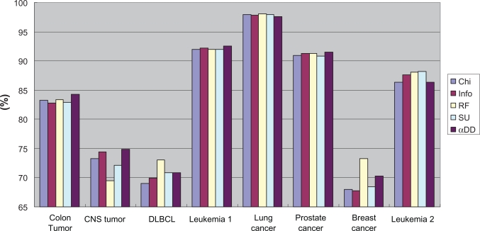
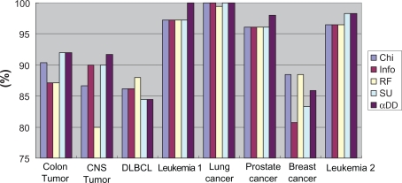
Figure 9 and Figure 10 contrast the average and best classification accuracies in all of the eight datasets for different feature selection methods. In the average accuracy, the α depended degree attained the best results in four datasets; in the best accuracy, the α depended degree attained the best results in six datasets. Taken together, the classification performance with the α depended degree are superior to or at least match that with the other four popular feature selection approaches.

Figure 9.

Contrast in average accuracy for different feature selection methods.

Figure 10.

Contrast in best accuracy for different feature selection methods.

Discussion and Conclusions

Because of the severe imbalance between feature numbers and instance numbers in microarray-based gene expression profiles, feature selection is essentially crucial in addressing the problem of molecular classification and identifying important biomarkers of cancer. To better molecularly classify cancers and detect significant marker genes, developing flexible and robust feature selection methods are of extreme importance. However, the conventional rough sets based feature selection method, the depended degree of attributes, was deficient in flexibility and robustness. Some indeed important genes may be missed just as their exceptional expression in a small number of samples if the depended degree criterion is used for gene selection. In contrast, we can avoid this kind of situations by the utility of the α depended degree criterion, which shows strong robustness by the flexible tuning of the α value. The α depended degree has been proven to be more efficient than the depended degree in gene selection through a series of classification experiments. Moreover, the α depended degree was comparable with the other established feature selection standards: chi-square, information gain, Relief-F and symmetric uncertainty, which was also demonstrated by the classification experiments. It should be noted that the classification results exhibited in this work might be biased towards higher estimates since the feature selections were ahead of LOOCV. However, the comparisons were generally just because all of the classification results were obtained based on the same procedures.

An interesting finding in the present study was that the α depended degree could reflect the inherent classification difficultness of one microarray dataset. Generally speaking, when the α depended degree was used for gene selection, if we could achieve the comparatively good classification accuracy in some cancerous microarray dataset, the corresponding α value would be relatively high, regardless of what classifier being used; otherwise, it would be relatively low. Moreover, once some dataset has been identified as difficultly-classified or easily-classified through the α depended degree, the dataset would be equally difficultly-classified or easily-classified using other gene selection methods, irrespective of classifiers. Therefore, if we want to gauge the difficultness of the cancer-related classification based on a new microarray dataset, the α depended degree can be used for addressing the problem. In fact, if excluding the quality factor of a cancerous microarray dataset, the classification difficultness of the dataset might reflect the essential biological properties of the relevant cancer.

The size of the selected gene subset by which a good classification is achieved is also an important factor in assessing the quality of a feature selection approach. In general, the accurate classification with a small size of genes is the better classification than that with a large number of genes. Our experiments did not exhibit substantial differences in the optimum gene numbers concerned with every feature selection method, partly because finding the optimum gene sizes need more delicate feature selection strategies instead of simply selecting a few top-ranked genes. One of our future work is to develop more favorable gene selection methods by merging the α depended degree based feature ranking with some heuristic strategies.

Table 1.

Summary of the eight gene expression datasets.

Dataset	# Original genes	Class	# Samples
Colon tumor	2000	negative/positive	62 (40/22)
CNS tumor	7129	class 1/class 0	60 (21/39)
DLBCL	7129	cured/fatal	58 (32/26)
Leukemia 1	7129	ALL/AML	72 (47/25)
Lung cancer	12533	MPM/ADCA	181 (31/150)
Prostate cancer	12600	tumor/normal	102 (52/50)
Breast cancer	24481	relapse/non-relapse	78 (34/44)
Leukemia 2	12582	ALL/MLL/AML	57 (20/17/20)

References

- 1.Golub TR, Slonim DK, Tamayo P, et al. Molecular classification of cancer: class discovery and class prediction by gene expression monitoring. Science. 1999;286(5439):531–7. doi: 10.1126/science.286.5439.531. [DOI] [PubMed] [Google Scholar]
- 2.Wang X, Gotoh O. Microarray-Based Cancer Prediction Using Soft Computing Approach. Cancer Informatics. 2009;7:123–39. doi: 10.4137/cin.s2655. [DOI] [PMC free article] [PubMed] [Google Scholar]
- 3.Li J, Wong L. Identifying good diagnostic gene groups from gene expression profiles using the concept of emerging patterns. Bioinformatics. 2002;18(5):725–34. doi: 10.1093/bioinformatics/18.5.725. [DOI] [PubMed] [Google Scholar]
- 4.Geman D, d’Avignon C, Naiman DQ, Winslow RL.Classifying gene expression profiles from pairwise mRNA comparisons Stat Appl Genet Mol Biol 20043:Article 19. [DOI] [PMC free article] [PubMed] [Google Scholar]
- 5.Alon U, Barkai N, Notterman DA, et al. Broad patterns of gene expression revealed by clustering analysis of tumor and normal colon tissues probed by oligonucleotide arrays. Proc Natl Acad Sci U S A. 1999;96(12):6745–50. doi: 10.1073/pnas.96.12.6745. [DOI] [PMC free article] [PubMed] [Google Scholar]
- 6.Pomeroy SL, Tamayo P, Gaasenbeek M, et al. Prediction of central nervous system embryonal tumour outcome based on gene expression. Nature. 2002;415(6870):436–42. doi: 10.1038/415436a. [DOI] [PubMed] [Google Scholar]
- 7.Shipp MA, Ross KN, Tamayo P, et al. Diffuse large B-cell lymphoma outcome prediction by gene-expression profiling and supervised machine learning. Nat Med. 2002;8(1):68–74. doi: 10.1038/nm0102-68. [DOI] [PubMed] [Google Scholar]
- 8.Gordon GJ, Jensen RV, Hsiao LL, et al. Translation of microarray data into clinically relevant cancer diagnostic tests using gene expression ratios in lung cancer and mesothelioma. Cancer Res. 2002;62(17):4963–7. [PubMed] [Google Scholar]
- 9.Singh D, Febbo PG, Ross K, et al. Gene expression correlates of clinical prostate cancer behavior. Cancer Cell. 2002;1(2):203–9. doi: 10.1016/s1535-6108(02)00030-2. [DOI] [PubMed] [Google Scholar]
- 10.van ‘t Veer LJ, Dai H, van de Vijver MJ, et al. Gene expression profiling predicts clinical outcome of breast cancer. Nature. 2002;415(6871):530–6. doi: 10.1038/415530a. [DOI] [PubMed] [Google Scholar]
- 11.Armstrong SA, Staunton JE, Silverman LB, et al. MLL translocations specify a distinct gene expression profile that distinguishes a unique leukemia. Nat Genet. 2002;30(1):41–7. doi: 10.1038/ng765. [DOI] [PubMed] [Google Scholar]
- 12.Pawlak Z. Rough sets. International Journal of Computer and Information Sciences. 1982;11:341–56. [Google Scholar]
- 13.Li D, Zhang W. Gene selection using rough set theory. The 1st International Conference on Rough Sets and Knowledge Technology. 2006:778–85. [Google Scholar]
- 14.Momin BF, Mitra S. Reduct generation and classification of gene expression data. First International Conference on Hybrid Information Technology. 2006:699–708. [Google Scholar]
- 15.Liu H, Li J, Wong L. A comparative study on feature selection and classification methods using gene expression profiles and proteomic patterns. Genome Inform. 2002;13:51–60. [PubMed] [Google Scholar]
- 16.Quinlan J. Induction of decision trees. Machine Learning. 1986;1:81–106. [Google Scholar]
- 17.Wang Y, Makedon FS, Ford JC, Pearlman J. HykGene: a hybrid approach for selecting marker genes for phenotype classification using microarray gene expression data. Bioinformatics. 2005;21(8):1530–7. doi: 10.1093/bioinformatics/bti192. [DOI] [PubMed] [Google Scholar]
- 18.Robnik-Sikonja M, Kononenko I. Theoretical and Empirical Analysis of ReliefF and RReliefF. Machine Learning Journal. 2003;53:23–69. [Google Scholar]
- 19.Fayyad UM, Irani KB. Multi-interval discretization of continuous-valued attributes for classification learning. The 13th International Joint Conference of Artificial Intelligence. 1993:1022–7. [Google Scholar]
- 20.Witten IH, Frank E. Data mining: practical machine learning tools and techniques. second edition. Morgan Kaufmann; 2005. [Google Scholar]
Associated Data
This section collects any data citations, data availability statements, or supplementary materials included in this article.