A Motion-Based Approach to Abdominal Clutter Reduction

Abstract

In ultrasound images, clutter is a noise artifact most easily observed in anechoic or hypoechoic regions. It appears as diffuse echoes overlying anatomical structures of diagnostic importance, obscuring tissue borders and reducing image contrast. A novel clutter reduction method for abdominal images is proposed, wherein the abdominal wall is displaced during successive-frame image acquisitions. A region of clutter distal to the abdominal wall was observed to move with the abdominal wall, and finite impulse response (FIR) and blind source separation (BSS) motion filters were implemented to reduce this clutter. The proposed clutter reduction method was tested in simulated and phantom data and applied to fundamental and harmonic in vivo bladder and liver images from 2 volunteers. Results show clutter reductions ranging from 0 to 18 dB in FIR-filtered images and 9 to 27 dB in BSS-filtered images. The contrast-to-noise ratio was improved by 21 to 68% and 44 to 108% in FIR- and BSS-filtered images, respectively. Improvements in contrast ranged from 4 to 12 dB. The method shows promise for reducing clutter in other abdominal images.

I. Introduction

In diagnostic ultrasound, clutter is a noise artifact that appears as diffuse echoes overlying structures or signals of interest. It is most easily observed in anechoic or hypoechoic regions of images, such as in the gall bladder or urinary bladder. clutter obscures diagnostic measurements and degrades image contrast [1].

Previous work identifies 2 primary mechanisms of clutter generation: off-axis scatter and reverberation [2]-[4]. Harmonic imaging, in which higher harmonics generated by nonlinear sound propagation through tissue are imaged, has been shown to reduce clutter due to both mechanisms [5]-[9]. a wide range of apodization [10], [11] and adaptive beamforming [12]-[14] techniques are aimed at reducing clutter due to off-axis scatterers. In this paper, we present a technique for reducing clutter due to abdominal wall reverberations.

Abdominal images can be modeled as containing 2 components, the abdominal wall and an underlying organ of interest, each contributing to image clutter via one of the primary clutter generation mechanisms. clutter due to off-axis scattering is proposed to arise from axial and elevational structures in and surrounding the organ of interest, while structures in the abdominal wall are proposed to cause clutter due to reverberation. Random (thermal) noise is also a potential source of clutter, however, clutter appears stationary in most applications, indicating that this clutter contribution is minimal and can be ignored.

The proposed clutter reduction method is well suited for abdominal images, where tissue-to-clutter ratios can range from 0 to 35 dB [1]. The method requires axial displacement of the abdominal wall during real-time imaging. Given the proposed model, clutter that arises from acoustic interaction (i.e., reverberation) in abdominal wall structures would experience similar displacements to the abdominal wall. This clutter is reduced by applying motion filters to the acquired images. The proposed method was tested in simulated, phantom, and in vivo images.

II. Methods

A. Field II Simulations

Field II [15], [16] was used to simulate clutter moving in the same direction and with the same velocity as the transducer, in the presence of stationary tissue, a necessary condition for the proposed clutter reduction method. When the motion is considered in a reference frame attached to the transducer, clutter moving with the transducer appears stationary, and stationary tissue appears to be moving. Thus, motion was simulated by incrementally displacing one speckle pattern representative of homogeneous tissue relative to a stationary speckle pattern representative of clutter.

The speckle patterns were created by insonifying a 6 cm (axial) × 5 cm (lateral) × 1 cm (elevation) phantom, containing at least 10 scatterers per resolution volume. Half of the scatterers in the phantom were given random amplitudes at random locations, representative of homogeneous tissue. The other scatterers were given random amplitudes weighted by a factor of 10(1 − z_p/6), where z_p is the axial distance (cm) from the proximal phantom surface. (Note: z_p is defined for 0 < z_p < 6 and z_p = z − 3, where z is the axial distance (cm) from the transducer surface.) This weighting function resulted in random scatterer amplitudes that linearly decreased with depth, similar to clutter noise in phantom and in vivo images [1]. The scatterers representing tissue were shifted 10 times in 0.1-mm increments toward the transducer to create motion relative to the simulated clutter. In addition to imaging tissue moving in the presence of stationary clutter, the tissue and clutter were imaged separately (i.e., all phantom scatterers represented either stationary clutter or moving tissue), and the resulting images were placed side by side.

The transducer parameters used in the simulations are listed in Table I. The axial transmit focus was 6 cm. Dynamic focusing was applied during receive beamforming, and Hanning window apodization was applied to the transmit and receive apertures.

Table I.

Transducer Parameters for Field II Simulations.

Parameter	Value
Number of elements (total)	192
Number of elements in subaperture	64
Element height	12 mm
Element width	0.314 mm
Kerf	0.014 mm
Center frequency	2.5 MHz
Sampling frequency	100 MHz
Fractional bandwidth	60%

B. Phantom and In Vivo Studies

A siemens Antares ultrasound scanner and Siemens CH6-2 curvilinear transducer (Siemens Medical Solutions USA, Inc., Issaquah, WA) were used to obtain phantom images and in vivo bladder and liver images from 2 male volunteers (ages 53 and 33). The scanner was operated in fundamental and harmonic imaging modes with transmit frequencies of 4.4 MHz and 2.5 MHz, respectively. The Axius Direct Ultrasound Research Interface (Siemens Medical Solutions USA, Inc., Issaquah, WA) was used to acquire raw radio frequency (RF) data without significant time-gain compensation and before the application of nonlinear processing steps. In harmonic imaging mode, the scanner implements the pulse inversion technique [17], [18], and harmonic RF data were obtained by summing the normal and inverted pulse-echo signals. To form B-mode images, the RF data obtained in fundamental or harmonic imaging mode were envelope detected, normalized to the brightest point, log-compressed, limited to a dynamic range of 45 dB, and then scan-converted. The axial sampling frequency was 40 MHz. The line densities were 0.25, 0.28, and 0.30 degrees per line, respectively, in phantom and in vivo liver images, in vivo fundamental bladder images, and in vivo harmonic bladder images. The pulse repetition frequencies were 7.2, 4.0, and 5.3 kHz, respectively. The frame rates were 25, 15, and 11 Hz, respectively. All image processing and analysis was implemented with Matlab (MathWorks Inc., Natick, MA) software.

A custom bladder phantom was created by submerging a water-filled balloon in a slurry solution of graphite, propanol, and water (RMI, now Gammex, Inc., Middleton, WI, SuperSpheres Model TM-C, discontinued by manufacturer). The ultrasonic transducer was placed in the slurry solution, with its imaging surface approximately 2 cm above the submerged balloon. A linear translation stage (Newport Motion Controller Model MM3000, Newport Corporation, Irvine, CA) was used to translate the transducer axially at a controlled velocity of 0.5 mm/s during real-time imaging. The distance the transducer traveled between successive images was 0.02 MM. To generate clutter that moved with the transducer, a wiry copper household scouring pad (ScrubIT Copper Scourers, Supply Plus, Inc. Newark, NJ) cut to 1 cm in thickness was placed at the transducer surface, the transducer and wire mesh were confined in A transducer bag containing enough water to provide acoustic coupling, and the motion experiment was repeated. In a previous study [1], the copper wire mesh was shown to generate clutter with similar characteristics to that of in vivo data (i.e., similar in magnitude, clutter magnitude greatest in near field, magnitude decreases with depth). This clutter is likely a reverberation artifact due to the highly reflective metallic material.

As a corollary to the phantom study, the abdominal wall was translated during successive-frame in vivo imaging of the bladder and liver. Abdominal wall motion was achieved by asking the volunteers to translate their abdominal muscles slowly while the hand-held transducer, resting and lightly supported on the abdominal skin, followed the motion. We anticipate that this motion allows the transducer, abdominal wall, and underlying clutter to move approximately in unison, while distal tissues remain stationary.

Displacement estimates for phantom and in vivo data were obtained by applying a normalized 2-D cross-correlation search method (i.e., speckle tracking) to successive frames of envelope-detected RF data [19]. Thus, while displacements are assumed to be axial along the probe axis, they were calculated along the beam axis. Given that a curvilinear probe was used for imaging, these 2 axes are similar for center beams (to the extent that the small angle approximation is valid) but not for outer beams.

The speckle-tracking kernel size was selected by minimizing false peaks in the cross correlation function, while maintaining acceptable resolution in displacement results. The optimal kernel size in fundamental bladder images was 25 × 5 pixels, and this kernel size was kept constant for all data. In scan-converted images, the kernel sizes correspond to 0.48 mm × 1.3° in phantom and in vivo liver data, 0.48 mm × 1.4° in the in vivo fundamental bladder images, and 0.48 mm × 1.5° in harmonic images. Kernels in one frame were compared with search regions of 100 × 10 pixels in the consecutive frame. In scan-converted images, the search region sizes correspond to 1.9 mm × 2.5° in phantom and in vivo liver data, 1.9 mm × 2.8° in the in vivo fundamental bladder images, and 1.9 mm × 3.0° in harmonic images. The search regions were centered about the kernel location. The speckle-tracking algorithm was not applied to kernels near the edges of the B-mode image where the search region extended beyond the image border.

C. Clutter Reduction with Motion Filters

Motion filters were applied to simulated, phantom, and in vivo images to remove clutter moving in the same direction and with the same velocity as the transducer (i.e., clutter that appears stationary to the transducer). The first filter was a conventional 1,−1 FIR motion filter, also known as a stationary echo canceller, wherein the RF echoes in one frame were subtracted from those in a consecutive frame to reject stationary RF echoes [20]. The second filter was a BSS filter, where basis functions were selected and/or rejected to reconstruct a filtered image [21]-[23].

BSS filtering was implemented by performing robust principal component analysis with the robpca function in the Matlab Library for Robust Analysis [24], [25]. This function requires an input data matrix with observations in its rows and variables in its columns. The input data matrix consisted of envelope-detected RF echoes taken from the same lateral position (observations) in consecutive images (variables). Basis function selection was based on the time and depth projections associated with the principal components of the input data [22], [23].

As described by Gallippi et al. [22], [23], a time projection yields the motion profile associated with a particular principal component, while the corresponding depth projection indicates the relative strength of that principal component at each axial position. For example, a time projection with zero slope represents a basis function associated with a stationary signal component, while a time projection with nonzero slope represents a basis function associated with a moving signal component. A depth projection with uniform amplitude represents a basis function associated with a signal component that is equally weighted at all axial positions. A depth projection with dominant magnitudes at specific axial positions indicates that the associated basis function is dominant at those positions. The relative amplitudes in a depth projection also depend on relative amplitudes in the associated signal component.

Although known to be true in simulated images and expected to be true in phantom images, axial motion was assumed to be uniform across the lateral dimension of in vivo images. Uniform motion implies similar basis functions for all lateral positions, thus, the selected basis function generated by one lateral position was used to filter all axial lines in an image. To reconstruct a BSS-filtered image, the data matrix of each axial line was projected onto the selected basis function, as described by

$$y_i=x_i{\mathit{vv}}^T,$$ (1)

where y_i is the ith lateral position (or ith axial line) of the filtered image, x_i is the data matrix of the ith lateral position in the original image, v is the eigenvector of the selected basis function, and v^T is the eigenvector transposed. The filtered RF lines were then normalized to the brightest point, log-compressed, and limited to a dynamic range of 45 dB. Scan conversion was the final step in filtered phantom and in vivo images.

Filter efficacy was demonstrated with contour maps illustrating magnitude differences between filtered and reference images. The contour maps were formed from envelope-detected RF echo data. The reference and motion-filtered data were low-pass filtered with a rectangular kernel of 151 × 15 pixels (2.9 mm × 3.8°, 2.9 mm × 4.2°, and 2.9 mm × 4.5° in scan-converted phantom and in vivo liver images, in vivo fundamental bladder images, and in vivo harmonic bladder images, respectively), and the pixel-wise ratio between resulting images was calculated.

The contrast in reference and filtered phantom and in vivo data was calculated using

$$\mathrm{C}=20\log {}_{10}\left(\frac{S_o}{S_i}\right),$$ (2)

where S_o and S_i are the mean envelope-detected RF data outside and inside a hypoechoic region, respectively. The contrast-to-noise ratio (CNR) in phantom and in vivo data was calculated using

$$\mathrm{CNR}=\frac{C}{20\log {}_{10}\left({\sigma }_o\right)},$$ (3)

where σ_o is the standard deviation of the envelope-detected RF data outside the hypoechoic region [26], [27].

III. Results

A. Field II Simulations

Fig. 1(a) shows the simulated images representing linearly decreasing clutter noise (left panel), homogeneous tissue in the presence of the clutter noise (middle panel), and tissue (right panel). A stationary echo canceller FIR filter was applied to the RF data in 2 consecutive frames, and the resulting image is shown in Fig. 1(b). The corresponding map of magnitude reductions in the filtered image is shown in Fig. 1(c). The left panel of this image shows the reduction of the clutter noise. Although the contour map was limited to 33 dB, the clutter in this region was reduced to zero, and the magnitude reduction in this region is infinity. In the second panel, the maximum reduction in the proximal region (3 to 3.5 cm) ranges from 21 to 24 dB. The distal region (8.5 to 9 cm) experiences 0- to 3-dB magnitude reduction. There are also regions with a 3- to 6-dB signal increase. In the third panel, the average signal increase is 4 dB. Notice that the magnitude increase at the bottom of the second panel is similar to the increase in the third panel.

Fig. 1.

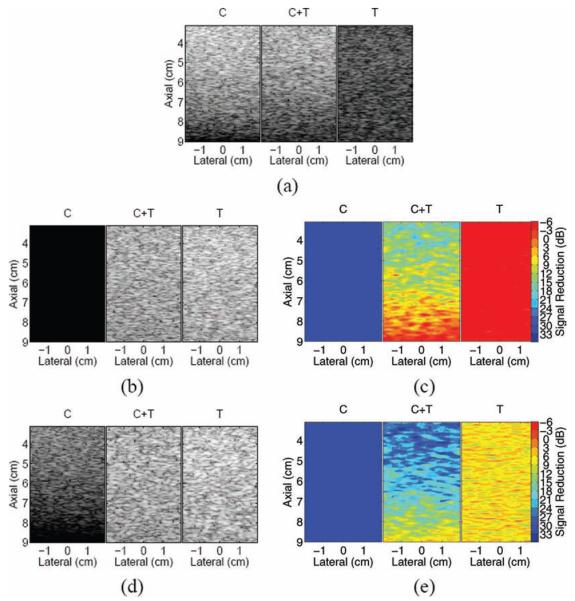
(a) Simulated phantom images showing clutter noise (C), clutter noise mixed with homogeneous tissue (C+T), and homogeneous tissue (T); (b) finite impulse response (FIR)–filtered images; (c) corresponding maps of magnitude reductions in FIR-filtered images; (d) blind source separation (BSS)–filtered images; and (e) corresponding maps of magnitude reductions in BSS-filtered images.

Robust principal component analysis was applied to the central lateral position of Fig. 1(a) (0 cm in C+T image), and Fig. 2(a) shows the first 4 time and depth projections, corresponding to the 4 most energetically significant principal components. The first depth projection has a slope that decreases with depth, much like the slope of the weighting function applied to the simulated clutter amplitudes. Similar results were achieved for the first depth projection of all lateral positions, as shown in Fig. 2(b). The first time projection has zero slope, indicating that this component of the signal is stationary (relative to the transducer). Similar results were achieved for the first time projections of all lateral positions, as shown in the top panel of Fig. 2(c). The described characteristics of the first depth and time projections provide strong evidence that the first basis function is associated with the simulated clutter.

Fig. 2.

Blind source separation time and depth projections of the simulated data: (a) the first 4 time (top) and depth (bottom) projections for the central lateral position; (b) average of the first depth projection of all lateral positions; and (c) average of the first (top) and second (bottom) time projections of all lateral positions. Error bars indicate one standard deviation.

The slope of the second time projection in Fig. 2(a) is constant and nonzero throughout, indicating that it is associated with uniform displacement, much like the incremental displacement applied to the simulated tissue. Similar results were achieved for the second time projections of all lateral positions, as shown in the bottom panel of Fig. 2(c). The described characteristics of the second time projection provide compelling evidence that the second basis function is associated with the simulated tissue motion. Given the characteristics of the third and fourth time and depth projections, their basis functions are likely associated with a mixture of stationary noise and tissue motion.

The second basis function generated by the central lateral position was determined to represent the most energetic nonstationary principal component. It was selected to filter all axial lines and reconstruct the BSS-filtered images shown in Fig. 1(d). A filter performance map of magnitude reductions in the filtered images is shown in Fig. 1(e). In the left panel of Fig. 1(e), the average reduction is 38 dB. In the middle panel, the map shows a maximum clutter reduction of 33 dB near the proximal phantom surface and a minimum reduction of 0 to 3 dB near the distal surface. In the right panel, the average reduction is 7 dB. Notice that the reductions at the top and bottom of the center panel are similar to the reductions of the left and right panels, respectively.

B. Phantom Experiments

Fig. 3(a) shows a B-mode image of the bladder phantom. The map of peak correlation coefficients between 2 successive frames acquired during transducer displacement is shown in Fig. 3(b). The frames were highly correlated in the regions surrounding the bladder, as well as inside the bladder, near the borders. There is less correlation inside the bladder, farther away from the borders, although the correlation coefficients are still high. Fig. 3(c) displays the corresponding axial displacement map, with displacement estimates shown relative to the transducer surface. In the reference frame of the transducer, the entire phantom is shown to have consistent motion toward the transducer.

Fig. 3.

Bladder phantom: (a) B-mode image; corresponding maps of (b) correlation coefficients and (c) axial displacements between 2 consecutive frames in the data set; (d) B-mode image of bladder phantom with clutter-generating layer placed at the transducer surface (the boxes show regions of interest used to calculate contrast and contrast-to-noise ratios in reference and filtered data); and corresponding maps of (e) correlation coefficients and (f) axial displacements between 2 consecutive frames in the data set. Displacements are relative to the transducer surface, where negative indicates motion toward the transducer and positive indicates motion away from the transducer.

Fig. 3(d) shows a B-mode image acquired when the clutter-generating wire mesh was placed between the transducer and the bladder, during simultaneous translation and successive-frame imaging. A map of the peak correlation coefficients between 2 successive frames is shown in Fig. 3(e). Similar to Fig. 3(b), the correlation coefficients are highest in the regions surrounding the bladder. The coefficients are also high inside the bladder, in a region extending well below the proximal wall. This highly correlated region inside the bladder corresponds to the clutter generated by the wire mesh, as seen in the B-mode image of Fig. 3(d). In the corresponding axial displacement map of Fig. 3(f), the region containing the wire mesh and the clutter region extending below the wire mesh have similar displacement estimates, displacements that are approximately 0 mm relative to the transducer. The surrounding regions have consistent upward motion relative to the transducer, similar to the displacements observed in Fig. 3(c).

The regions with lower correlation coefficients (approximately 0.8) in Fig. 3(e) have discontinuous displacement estimates in the corresponding axial displacement map of Fig. 3(f) (e.g., the region surrounding axial position 1 cm, lateral position −3 cm). This type of displacement is not consistent with the transducer's uniform motion toward the bladder. Therefore, regions showing such random motion are interpreted as regions of indeterminate displacements.

Results of the FIR filter applied to 2 consecutive frames of the phantom image with the wire mesh are shown in Figs. 4(a) and (b). Reductions of 6 to 18 dB are seen in the clutter region inside the bladder cavity. Reductions of 18 to 27 dB are seen in the proximal regions occupied by the wire mesh (0 to 1 cm) and distal to the wire mesh (1 to 3 cm). The regions with reduced magnitudes were shown to have approximately zero displacement (relative to the transducer) in Fig. 3(f). The regions of interest (ROIs) shown in Fig. 3(d) were used to calculate contrast and CNR in the reference and filtered phantom images. There is a 7-dB contrast increase and 42% CNR increase in the FIR-filtered image (see Table II).

Fig. 4.

Single frame results of the motion filters applied to the phantom data: (a) finite impulse response (FIR)–filtered image; (b) corresponding map of regional magnitude reductions in the FIR-filtered image, when compared with the reference image in Fig. 3(d); (c) blind source separation (BSS)–filtered image; and (d) corresponding map of regional magnitude reductions in the BSS-filtered image, when compared with the reference image in Fig. 3(d).

Table II.

Contrast and Contrast-to-Noise Ratios (CNR) in Reference and Filtered Images.

	Contrast (dB)	CNR
Bladder phantom images
Reference	23.2	0.50
FIR-filtered	30.5	0.71
BSS-filtered	32.1	0.72
In vivo bladder images
Reference (fundamental)	12.1	0.26
FIR-filtered	17.4	0.34
BSS-filtered	19.7	0.54
Reference (harmonic)	15.8	0.38
FIR-filtered	19.5	0.46
BSS-filtered	22.0	0.59
In vivo gall bladder images
Reference	16.9	0.31
FIR-filtered	29.4	0.52
BSS-filtered	26.0	0.52

FIR = finite impulse response; BSS = blind source separation.

The BSS filter results shown in Figs. 4(c) and (d) are similar to the FIR filter results. The central lateral position (0 cm) was used to generate basis functions for image reconstruction. Depth projections with large amplitudes in the distal bladder wall region and time projections with decreasing slopes represented the principal components associated with motion (relative to the transducer). The first basis function had the steepest time projection slope (i.e., it represented the most energetic component associated with motion), and it was therefore selected to reconstruct the filtered image. Reductions of 3 to 18 dB are seen in the clutter region inside the bladder cavity. Reductions of 18 to 21 dB are seen in the proximal regions occupied by the wire mesh (0 to 1 cm) and distal to the wire mesh (1 to 3 cm). Similar to FIR-filtered images, the regions with reduced magnitudes in the BSS-filtered images were shown to have approximately zero displacement (relative to the transducer) in Fig. 3(f). There is a 9-dB contrast increase and 44% CNR increase in the BSS-filtered image (see Table II).

The proximal bladder wall is not visualized in the filtered B-mode images of Figs. 4(a) and (c), because the gain in this region of the original B-mode image was minimized to achieve uniform image brightness; see Fig. 3(d). However, when the dynamic range (currently 45 dB) was increased above 60 dB in the filtered images, the proximal bladder wall was more apparent, but so was the clutter inside the bladder. The filter performance maps of Figs. 4(b) and (d) reinforce this observation, because the region representing the proximal bladder wall has a reduction that is 3 to 6 dB greater than the region representing the bladder interior.

C. In Vivo Experiment: Bladder Images

Fig. 5(a) shows a fundamental bladder image from Volunteer 1, with a manually estimated outline of the bladder wall superimposed on the image. Fig. 5(d) shows displacement estimates between 2 consecutive bladder images acquired during axial displacement of the abdominal wall. The displacement of the abdominal wall is approximately 0 mm relative to the transducer, confirming the anticipated outcome that the abdominal wall and the transducer moved approximately in unison. Similar to the phantom experiment with the wire mesh, the displacement map shows that clutter in the proximal bladder cavity was also moving with the abdominal wall (displacement estimates of approximately 0 mm relative to the transducer). The lateral and distal bladder walls and adjacent tissue have displacements of approximately 0.1 mm relative to the transducer. These results support the hypotheses about the applied motion that the transducer, abdominal wall, and underlying clutter move approximately in unison while distal tissues remain stationary.

Fig. 5.

(a) Fundamental and (g) harmonic B-mode bladder images from Volunteer 1, with estimated bladder outlines superimposed. (The images were acquired at different times, hence the different appearances.) The boxes show regions of interest (ROI) used to calculate contrast and contrast-to-noise ratios in reference and filtered data. (b) Finite impulse response (FIR)– and (c) blind source separation (BSS)–filtered fundamental images and corresponding maps of (d) axial displacements between 2 consecutive frames, (e) FIR filter performance, and (f) BSS filter performance; (h) FIR- and (i) BSS-filtered harmonic images and corresponding maps of (j) axial displacements, (k) FIR filter performance, and (l) BSS filter performance. Axial displacements are relative to the transducer surface, where negative indicates motion toward the transducer and positive indicates motion away from the transducer. Axial displacement maps show ROI in the abdominal wall, clutter distal to the abdominal wall, and the distal bladder wall. These ROI were used to calculate average displacements in all consecutive frames of the data set (see Fig. 6).

Fig. 5(g) shows a harmonic bladder image from volunteer 1, with a manually estimated outline of the bladder wall superimposed on the image. A corresponding map of axial displacements between 2 consecutive harmonic images is shown in Fig. 5(j). Although the 2-D displacement maps in Figs. 5(d) and (j) show displacements between 2 consecutive frames, similar results were achieved in all consecutive frames of each data set, as shown in Fig. 6. Similar results were achieved in fundamental and harmonic bladder images from Volunteer 2 (images not shown).

Fig. 6.

Average axial displacements of select regions in displacement maps of consecutive fundamental (a) and harmonic (b) images. The regions of interest used to calculate average displacements are shown in Figs. 5(d) and (j), respectively. Displacements are relative to the transducer surface, where negative indicates motion toward the transducer and positive indicates motion away from the transducer.

It is important to note that the displacement results of Figs. 5 and 6 were obtained while the abdominal muscles were relaxed (i.e., the muscles were not tensed/tightened while being translated). With the abdominal muscles tightened during translation (results not shown), instead of having 0 mm displacement in the proximal bladder cavity region, displacement estimates in this region were more spatially random, much like those at 6 to 9 cm in the hypoechoic bladder region of Fig. 5(d). Additionally, the distal and lateral bladder wall regions contained displacement estimates near 0.1 mm, and the proximal bladder wall was shown to have similar axial displacements to the lateral and distal bladder walls.

Results of the FIR filter applied to 2 consecutive fundamental images from volunteer 1 are shown in Fig. 5(b) and (e). Clutter reductions of 3 to 9 dB are seen in the proximal bladder cavity (2 to 6 cm). Results of the FIR applied to 2 consecutive harmonic images are shown in Figs. 5(h) and (k), where clutter reductions of 0 to 12 dB are seen in the proximal bladder cavity (3 to 6 cm). The clutter regions with reduced magnitudes in FIR-filtered fundamental and harmonic images were shown to have approximately zero displacement in Fig. 5(d) and (j), respectively. In corresponding filter performance maps, shown in Figs. 5(e) and (k), the abdominal wall experiences a magnitude reduction ranging from 3 to 18 dB (with negligible regions showing 21- to 24-db reduction), while the distal and lateral walls experience a signal increase of 3 to 6 dB. The contrasts are improved by 5 dB in the FIR-filtered fundamental image and 4 dB in the FIR-filtered harmonic image, while the CNRs are improved by 31% and 21%, respectively (see Table II).

Results of the BSS filter applied to fundamental and harmonic images are shown in Fig. 5(c) and (i), respectively. A central lateral position (0 cm and −0.7 cm, respectively) was used to generate basis functions for image reconstruction. Depth projections with large-amplitude near-field signals and time projections with slopes close to zero represented principal components associated with stationary clutter (relative to the transducer). Depth projections with large amplitudes in the distal bladder wall region and time projections with decreasing slopes represented the principal components associated with motion (relative to the transducer). The second basis function had the steepest time projection slope and was selected for image reconstruction.

As shown in Figs. 5(f) and (l), respectively, clutter in the proximal bladder cavity was reduced by 18 to 24 dB in the filtered fundamental image and 12 to 14 dB in the filtered harmonic image. The clutter regions that experienced magnitude reductions were shown to be approximately stationary relative to the transducer, as demonstrated in Figs. 5(d) and (j). In the fundamental BSS-filtered image, the abdominal wall experienced similar reductions to the proximal clutter region inside the bladder. In the harmonic BSS-filtered image, the abdominal wall was reduced by 15 to 21 dB. The tissue surrounding the lateral and distal bladder walls in fundamental and harmonic BSS-filtered images experienced reductions of 6 to 15 dB and 3 to 9 dB, respectively, similar to the distal clutter region inside the bladder. The contrast improvements in the BSS-filtered fundamental and harmonic images were 8 dB and 6 dB, respectively, while the CNRs were increased by 108% and 45%, respectively (see Table II).

D. In Vivo Experiment: Liver Images

A fundamental B-mode image of the gall bladder and surrounding liver tissue of volunteer 1 is shown in Fig. 7(a). Successive-frame liver images were acquired during axial translation of the abdominal wall. Displacement estimates between 2 consecutive images are shown in Fig. 7(b). The abdominal wall and a region distal to the abdominal wall are shown to be stationary relative to the transducer, while the distal tissues are shown to move toward the transducer. The stationary region is similar to that of in vivo bladder images from the same volunteer. Furthermore, the stationary region is juxtaposed to the moving region in the liver image, whereas the 2 regions are separated by a region of random displacements in bladder images.

Fig. 7.

Results of the motion-based clutter reduction method applied to an in vivo liver: (a) fundamental liver image from volunteer 1; the boxes show regions of interest used to calculate contrast and contrast-to-noise ratio in reference and filtered data; (b) map of axial displacements between 2 consecutive frames in the image sequence; (c) finite impulse response–filtered image and (d) corresponding map of regional magnitude reductions in the filtered image; and (e) blind source separation–filtered image and (f) corresponding map of regional magnitude reductions in the filtered image.

An FIR filter was applied to 2 consecutive frames in the data set. The filtered image is shown in Fig. 7(c), and the corresponding filter performance map is shown in Fig. 7(d). Regions that were shown to move with the transducer were reduced by 3 to 24 dB in the filtered image. Most of the distal tissues experienced a 0 to 3 dB signal increase. There is a 12-dB contrast increase and 68% CNR increase in the FIR-filtered image (see Table II).

The BSS-filtered image is shown in Fig. 7(e). The lateral position of the brightest point inside the gall bladder image (−0.2 cm) was used to generate the basis functions for image reconstruction. The second basis function had the steepest time projection slope, and it was selected for image reconstruction. As shown in Fig. 7(f), the clutter in the gall bladder is reduced by 19 to 21 dB. The region that was shown to move with the abdominal wall, as shown in Fig. 7(b), is reduced by 12 to 21 dB (disregarding the small 3- to 9-dB regions to the right of the image). There is a 9-dB contrast increase and 68% CNR increase in the BSS-filtered image (see Table II).

IV. Discussion

A. Implications for Clutter Reduction in Abdominal Images

Clutter noise is apparent in the hypoechoic regions of the bladder and gall bladder (previous literature states that these regions should be hypoechoic or anechoic in the absence of clutter [28], [29]). Such hypoechoic regions are not always present in abdominal images of diagnostic interest. The tissue may be completely echogenic throughout the field of view, allowing clutter noise to be less noticeable. The simulation results of Fig. 2 demonstrate that the FIR and BSS filters are able to reduce stationary clutter in the midst of moving tissue signals that are completely echogenic. These results imply that the proposed motion-based clutter reduction method can be implemented in several types of abdominal images, with or without hypoechoic regions for easy visualization of clutter reductions.

The inclusion of the wire mesh in phantom images produced clutter distal to the mesh, which moved with the transducer during axial translation; see Fig. 3 (f). When the mesh was absent, the clutter seen in the anechoic region of the phantom image did not move with the transducer; see Fig. 3 (c). The clutter that moved with the transducer is suspected to arise from sound reverberation in the wire mesh. It was reduced, as shown in Fig. 4, via the proposed clutter reduction method.

Similarly, in the hypoechoic regions of in vivo bladder and liver images, the displacement maps of Figs. 5 and 7 show that there is a persistent region of clutter distal to the abdominal wall that moved at the same rate as the transducer and the displaced abdominal wall. This clutter is suspected to arise from acoustic interactions within the abdominal wall, such as sound reverberation. This clutter region was not as prevalent in displacement maps when the experiment was performed with tightened abdominal muscles, further supporting the hypothesis that a major source of this clutter is reverberation in abdominal tissue. A region of similar shape and size appears in the hypoechoic region of bladder images from the same volunteer—e.g., compare Figs. 5(d) and 7(b)—as well as in the anechoic region of the phantom image with the wire mesh; see Fig. 3 (f). This region of clutter is believed to overlay a large portion of the in vivo liver image (not just the hypoechoic region) and is most likely present in other abdominal images.

Additional confirmation that clutter overlays abdominal images is found in the displacement data of in vivo images. Although random displacements were primarily seen at the boundary separating stationary and moving signals in hypoechoic regions of bladder images, as seen in Figs. 5(d) and (j), such random displacements did not separate the 2 motions in the liver image; see Fig. 7 (b). Instead, the regions containing the 2 motions were juxtaposed, and the boundary separating them occurred in the echogenic tissue region distal to the gall bladder. Thus, the echogenic regions distal to the gall bladder (as well as the echogenic regions surrounding the gall bladder) are either due to tissue (moving regions) or clutter overlying the tissue (stationary regions). This is most likely true for echogenic regions in other abdominal images. As demonstrated with simulated and in vivo liver data, the proposed clutter reduction method is feasible in such echogenic environments.

B. Motion Filter Advantages and Limitations

The expected performance of the FIR and BSS motion filters is confirmed by simulation results. When applied to the left panel of Fig. 1(a) (the panel containing only clutter noise), the FIR filter successfully cancels stationary echoes, reducing the magnitude to zero, while the BSS filter reduces clutter magnitude by 38 dB. When applied to the right panel of Fig. 1(a) (the panel containing only tissue), the filters have similar responses to the distal region (8.5 to 9 cm) of respective center panels, confirming the similarity of these regions and demonstrating repeatable filter performance. In the FIR-filtered image, the distal region of the center panel experiences a magnitude reduction of 0 to 3 dB, which is expected given that the clutter in this region has approximately zero amplitude. Furthermore, the proximal region (3 to 3.5 cm) of this FIR-filtered image experiences a magnitude reduction ranging from 18 to 24 dB, which is close to expected, given that the average magnitude of the clutter noise in this region is approximately 10 times (20 dB) greater than the average magnitude of the simulated tissue. The BSS-filtered image has greater reductions than the FIR-filtered image, as discussed in greater detail later in this section. The center panels of both FIR- and BSS-filtered images have the greatest reductions in the near-field and decreasing reductions with depth.

Similar to the center panel of filtered simulation images, the near-field regions in phantom and in vivo images experience the greatest clutter reduction. The near-field reduction is most dramatic in the filtered phantom images, as seen in Figs. 4(a) and (c), where both clutter and tissue signal are removed. Reduction of the tissue signal in the phantom data indicates that the proposed BSS and FIR filters reduce slowly moving tissue as well as stationary echoes (relative to the transducer). However, when applied to the in vivo data, the filters yield a more realistic representation of near-field structures.

Considering that the primary goal of these filters is to reduce echoes that are stationary relative to the transducer, it is expected that the wire mesh (phantom images) and the abdominal wall (in vivo images) would be reduced in the filtered images, because these structures were moving with the transducer. Although this goal is beneficial when considering clutter that moves with the wire mesh and abdominal wall, it results in the reduction of these structures. To circumvent this issue, one might consider cropping near-field structures out of the image before motion filtering, then adjoining the cropped portion to the filtered image afterwards. Nevertheless, when imaging structures at depth, near-field abdominal layers are often unimportant.

The simulated and in vivo FIR-filtered images show increased signal magnitudes in regions that are moving relative to the transducer. Signal increases are not observed in the phantom FIR-filtered images. The increase is likely due to the subtraction of RF lines with large axial shifts (shifts in simulated and in vivo data are an order of magnitude larger than shifts in phantom data). For example, if identical regions in the shifted RF lines have the same magnitude but opposite signs, subtraction would yield a signal that is twice the magnitude of the original signal. This situation may be encountered when RF lines are shifted by half the transmit pulse wavelength, λ, which occurs when there is a displacement of λ/4 relative to the transducer. Axial displacements are comparable to λ/4 in simulated and in vivo images and smaller than λ/4 in phantom images (λ/4 = 0.15 mm in simulation and harmonic images, λ/4 = 0.088 mm in fundamental images). Thus, large (~λ/4) axial displacements are likely the reason for the 3- to 6-dB signal increases observed in FIR filter performance maps of simulated and in vivo data.

Although the performance of FIR and BSS filters is similar in phantom images, the reductions in simulated and in vivo BSS-filtered images are greater than those in respective FIR-filtered images. The greater reductions in BSS-filtered simulation and in vivo images are likely due to the fact that the second principal components were used to reconstruct simulated and in vivo data, while the first principal component was used to reconstruct the phantom image. Because higher-order principal components contain less of the original image energy [21], [23], it is expected that images reconstructed with the second principal component would contain less energy than images reconstructed with the first principal component. Thus, images reconstructed with higher order principle components experience signal attenuation and are expected to contain decreased signal-to-noise ratios when significant levels of random (thermal) noise are present.

Despite the greater reductions seen in BSS filter performance maps of simulated and in vivo images, the relative clutter reductions in BSS filter performance maps are comparable to relative clutter reductions in corresponding FIR filter performance maps. This explains why some BSS filter performance maps show greater reductions than corresponding FIR filter performance maps, yet the clutter seen in corresponding FIR- and BSS-filtered B-mode images is similar; e.g., compare Fig. 5(b) with Fig. 5(c).

Previous studies have shown that harmonic imaging reduces clutter in bladder images by 15 ± 3 dB (average of 5 volunteers) [1]. Clutter reductions achieved with the BSS filter applied to in vivo fundamental images is comparable to clutter reductions achieved with harmonic imaging, while the FIR filter yields less clutter reductions. The FIR and BSS filters applied to harmonic images were shown to reduce clutter in the harmonic images, suggesting that higher levels of clutter reduction may be achieved when this motion-based approach is applied to harmonic images. Note that motion artifacts in the harmonic data are negligible, given the high pulse repetition frequency (5.3 kHz) compared with the smaller frame rate (11 Hz).

The contrast in filtered phantom and in vivo images was increased by 4 to 12 dB. The CNR was improved by 21 to 68% in FIR-filtered images and 44 to 108% in BSS-filtered images. Given the limited number of volunteers, performance assessment in a broad range of individuals is unavailable and beyond the scope of this paper. However, similar contrast and CNR improvements are likely if the proposed clutter reduction method were applied to other abdominal images.

Real-time implementation of the proposed method is more feasible for the 1,−1 FIR filter because it only requires a lag of one frame and a subtraction operation. On the other hand, the BSS filter must be implemented over several frames, and appropriate basis functions must be identified before filter implementation. The speed of the processor and the size of data sets are also important factors in determining the real-time feasibility of BSS filtering.

V. Conclusion

The proposed clutter reduction method requires axial displacement of the abdominal wall during real-time imaging. The method assumes uniform displacement of the abdominal wall and associated clutter, both of which appear stationary to the imaging transducer. FIR and BSS motion filters were applied to reduce the stationary clutter. The method was tested in simulated, phantom, and in vivo images. The results demonstrate that the FIR and BSS filters are able to isolate and reduce clutter noise in hypoechoic and echogenic regions moving relative to the transducer. Clutter reductions ranged from 12 to 24 dB and contrast improvements ranged from 4 to 12 dB. The CNR was improved by 21 to 68% in FIR-filtered images and 44 to 108% in BSS-filtered images. The successes achieved in simulated, phantom, and in vivo images are promising evidence of this method's potential for reducing clutter in a vast array of abdominal images.

Biographies

Muyinatu A. Lediju was born August 3, 1984, in Brooklyn, NY. She studied at the Massachusetts Institute of Technology, Cambridge, MA, where she earned her B.S. degree in mechanical engineering with a minor in biomedical engineering in 2006. She is currently pursuing her Ph.D. degree in biomedical engineering at Duke University, Durham, NC. Her research interests include mechanical design of medical devices, medical imaging, ultrasonic clutter, multidimensional motion tracking, and echocardiography.

Michael J. Pihl, born in 1983, is currently enrolled as an M.Sc. student in biomedical engineering at the Technical University of Denmark and the University of Copenhagen. He writes his master's thesis at the Center for Fast Ultrasound Imaging (CFU) on blood vector velocity imaging. In 2007, he spent seven months at the Biomedical Engineering Department at Duke University, Durham, NC, researching ultrasonic clutter. His research interests include medical imaging, blood velocity estimation, and signal processing.

Stephen J. Hsu was born in Huntsville, AL, in 1980. He received his B.S.E. degree in biomedical and electrical engineering from Duke University, Durham, NC, in 2001 and his Ph.D. degree in Biomedical Engineering from Duke University in 2009. His research interests include acoustic radiation force impulse imaging and cardiac ultrasound imaging.

Jeremy J. Dahl was born in Ontonagon, Michigan, in 1976. He received the B.S. degree in electrical engineering from the University of Cincinnati, Cincinnati, OH, in 1999. He received the Ph.D. degree in biomedical engineering from Duke University in 2004. He is an assistant research professor in the Department of Biomedical Engineering at Duke University. He is currently researching adaptive ultrasonic imaging systems and radiation force imaging methods.

Caterina M. Gallippi earned a B.S.E. degree in electrical engineering and a certificate in engineering biology from Princeton University in 1998. She completed her Ph.D. degree in biomedical engineering at Duke University in 2003 with a focus on ultrasonic imaging. Dr. Gallippi is currently an assistant professor in the joint Department of Biomedical Engineering at the University of North Carolina-chapel Hill and North Carolina State University. Her research interests include radiation force imaging, adaptive signal filtering, multidimensional motion tracking, and targeted contrast imaging.

Gregg E. Trahey (S'83–M'85) received the B.G.S. and M.S. degrees from the University of Michigan, Ann Arbor, MI, in 1975 and 1979, respectively. He received the Ph.D. degree in biomedical engineering in 1985 from Duke University, Durham, NC. He served in the Peace Corps from 1975 to 1978, and was a project engineer at the Emergency Care Research Institute in Plymouth Meeting, PA, from 1980 to 1982. He is a professor with the Department of Biomedical Engineering, Duke University. He is conducting research in adaptive phase correction, radiation force imaging methods, and 2-D flow imaging in medical ultrasound.

References

- 1.Lediju MA, Pihl MJ, Dahl JJ, Trahey GE. Quantitative assessment of the magnitude, impact, and spatial extent of ultrasonic clutter. Ultrason. Imaging. 2008 Jul.30(3):151–168. doi: 10.1177/016173460803000302. [DOI] [PMC free article] [PubMed] [Google Scholar]
- 2.Lediju MA, Pihl MJ, Hsu SJ, Dahl JJ, Gallippi CM, Trahey GE. Magnitude, origins, and reduction of abdominal ultrasonic clutter. Proc. Ultrasonics Symp. 2008:50–53. [Google Scholar]
- 3.Dahl JJ, Pinton GF, Lediju MA, Trahey GE. Simulation and experimental analysis of ultrasonic clutter in fundamental and harmonic imaging. Proc. SPIE. 2009;7265(726509) [Google Scholar]
- 4.Carson PL, Oughton TV. A modeled study for diagnosis of small anechoic masses with ultrasound. Radiology. 1977 Mar.122:765–771. doi: 10.1148/122.3.765. [DOI] [PubMed] [Google Scholar]
- 5.Duck FA. Nonlinear acoustics in diagnostic ultrasound. Ultrasound Med. Biol. 2002 Jan.28(1):1–18. doi: 10.1016/s0301-5629(01)00463-x. [DOI] [PubMed] [Google Scholar]
- 6.Lencioni R, Cioni D, Bartolozzi C. Tissue harmonic and contrast-specific imaging: Back to gray scale in ultrasound. Eur. Radiol. 2002 Jan.12(1):151–165. doi: 10.1007/s003300101022. [DOI] [PubMed] [Google Scholar]
- 7.Thomas JD, Rubin DN. Tissue harmonic imaging: Why does it work? J. Am. Soc. Echocardiogr. 1998 Aug.11(8):803–808. doi: 10.1016/s0894-7317(98)70055-0. [DOI] [PubMed] [Google Scholar]
- 8.Tranquart F, Grenier N, Eder V, Pourcelot L. Clinical use of ultrasound tissue harmonic imaging. Ultrasound Med. Biol. 1999 Jul.25(6):889–894. doi: 10.1016/s0301-5629(99)00060-5. [DOI] [PubMed] [Google Scholar]
- 9.Averkiou MA. Tissue harmonic imaging. Proc. IEEE Ultrasonics Symp. 2000;2:1563–1572. [Google Scholar]
- 10.Stankwitz HC, Dallaire RJ, Fienup JR. Nonlinear apodization for sidelobe control in SAR imagery. IEEE Trans. Aerosp. Electron. Syst. 1995;31(1):267–279. [Google Scholar]
- 11.Seo CH, Yen JT. Sidelobe suppression in ultrasound imaging using dual apodization with crosscorrelation. IEEE Trans. Ultrason. Ferroelectr. Freq. Control. 2008 Oct.55(10):2198–2210. doi: 10.1109/TUFFC.919. [DOI] [PMC free article] [PubMed] [Google Scholar]
- 12.Viola F, Ellis MA, Walker WF. Time-domain optimized near-field estimator for ultrasound imaging: Initial development and results. IEEE Trans. Med. Imaging. 2008 Jan.27(1):99–110. doi: 10.1109/TMI.2007.903579. [DOI] [PMC free article] [PubMed] [Google Scholar]
- 13.Mann JA, Walker WF. A constrained adaptive beamformer for medical ultrasound: Initial results. Proc. IEEE Ultrasonics Symp. 2002;2:1807–1810. [Google Scholar]
- 14.Vignon F, Burcher MR. Capon beamforming in medical ultrasound imaging with focused beams. IEEE Trans. Ultrason. Ferroelectr. Freq. Control. 2008 Mar.55(3):619–628. doi: 10.1109/TUFFC.2008.686. [DOI] [PubMed] [Google Scholar]
- 15.Jensen JA, Svendsen NB. Calculation of pressure fields from arbitrarily shaped, apodized, and excited ultrasound transducers. IEEE Trans. Ultrason. Ferroelectr. Freq. Control. 1992 Mar.39:262–267. doi: 10.1109/58.139123. [DOI] [PubMed] [Google Scholar]
- 16.Jensen JA. Field: A program for simulating ultrasound systems. Med. Biol. Eng. Comput. 1996;34:351–353. [Google Scholar]
- 17.Ma Q, Ma Y, Gong X, Zhang D. Improvement of tissue harmonic imaging using the pulse-inversion technique. Ultrasound Med. Biol. 2005 Jul.31(7):889–894. doi: 10.1016/j.ultrasmedbio.2005.03.006. [DOI] [PubMed] [Google Scholar]
- 18.Simpson DH, Chin CT, Burns PN. Pulse inversion doppler: A new method for detecting nonlinear echoes from microbubble contrast agents. IEEE Trans. Ultrason. Ferroelectr. Freq. Control. 1999 Mar.46(2):372–382. doi: 10.1109/58.753026. [DOI] [PubMed] [Google Scholar]
- 19.Pinton GF, Dahl JJ, Trahey GE. Rapid tracking of small displacements with ultrasound. IEEE Trans. Ultrason. Ferroelectr. Freq. Control. 2006 Jun.53(6):1103–1117. doi: 10.1109/tuffc.2006.1642509. [DOI] [PubMed] [Google Scholar]
- 20.Jensen JA. Stationary echo canceling in velocity estimation by time-domain cross-correlation. IEEE Trans. Med. Imag. 1993;12(3):471–477. doi: 10.1109/42.241874. [DOI] [PubMed] [Google Scholar]
- 21.Gallippi CM, Trahey GE. Adaptive clutter filtering via blind source separation for two-dimensional ultrasonic blood velocity measurement. Ultrason. Imaging. 2002 Oct.24(4):193–214. doi: 10.1177/016173460202400401. [DOI] [PubMed] [Google Scholar]
- 22.Gallippi CM, Nightingale KR, Trahey GE. BSS-based filtering of physiological and ARFI-induced tissue and blood motion. Ultrasound Med. Biol. 2003 Nov.29(11):1583–1592. doi: 10.1016/j.ultrasmedbio.2003.07.002. [DOI] [PubMed] [Google Scholar]
- 23.Gallippi CM. Dept. of Biomedical Engineering. Duke University; Durham, NC: 2003. Blind source separation for selective tissue motion measurement in ultrasonic imaging. Ph.D. dissertation. [Google Scholar]
- 24.Verboven S, Hubert M. LIBRA: A MATLAB library for robust analysis. Chemom. Intell. Lab. Syst. 2005;75(2):127–136. [Google Scholar]
- 25.Hubert M, Rousseeuw PJ, Vanden Branden K. ROBPCA: A new approach to robust principal component analysis. Techno-metrics. 2005;47(1):64–79. [Google Scholar]
- 26.Karaman M, Li PC, O'Donnell M. Synthetic aperture imaging for small scale systems. IEEE Trans. Ultrason. Ferroelectr. Freq. Control. 1995 May;42(3):429–442. [Google Scholar]
- 27.Li PC, O'Donnell M. Improved detectability with blocked element compensation. Ultrason. Imaging. 1994 Jan.16(1):1–18. doi: 10.1177/016173469401600101. [DOI] [PubMed] [Google Scholar]
- 28.Ortega D, Burns PN, Hope Simpson D, Wilson SR. Tissue harmonic imaging is it a benefit for bile duct sonography? AJR Am. J. Roentgenol. 2001 Mar.176(3):653–659. doi: 10.2214/ajr.176.3.1760653. [DOI] [PubMed] [Google Scholar]
- 29.Yarmenitis SD. Ultrasound of the gallbladder and the biliary tree. Eur. Radiol. 2002 Feb.12(2):270–282. doi: 10.1007/s00330-001-1251-8. [DOI] [PubMed] [Google Scholar]