

Summary
Image-based, high throughput genome-wide RNA interference (RNAi) experiments are increasingly carried out to facilitate the understanding of gene functions in intricate biological processes. Automated screening of such experiments generates a large number of images with great variations in image quality, which makes manual analysis unreasonably time-consuming. Therefore, effective techniques for automatic image analysis are urgently needed, in which segmentation is one of the most important steps. This paper proposes a fully automatic method for cells segmentation in genome-wide RNAi screening images. The method consists of two steps: nuclei and cytoplasm segmentation. Nuclei are extracted and labelled to initialize cytoplasm segmentation. Since the quality of RNAi image is rather poor, a novel scale-adaptive steerable filter is designed to enhance the image in order to extract long and thin protrusions on the spiky cells. Then, constraint factor GCBAC method and morphological algorithms are combined to be an integrated method to segment tight clustered cells. Compared with the results obtained by using seeded watershed and the ground truth, that is, manual labelling results by experts in RNAi screening data, our method achieves higher accuracy. Compared with active contour methods, our method consumes much less time. The positive results indicate that the proposed method can be applied in automatic image analysis of multi-channel image screening data.
Keywords: active contour, automatic image segmentation, constraint factor, fluorescent microscopy, genome-wide screening, graph cut, morphological algorithm, RNAi
Introduction
In recent years, the understanding of gene functions in various biological phenomena is becoming increasingly important. The function of agene can be determined by inspecting changes in a biological process caused by the absence of the gene. By addition of gene-specific double-stranded RNA (dsRNA), specific and reproducible loss-of-function phenotypes can be mimicked to ‘knock out’ target gene function. This process is known as RNA-interference (RNAi). Process of RNAi can be screened by automated fluorescence microscopy. The high-throughput images help biologists to decode complex cellular processes and determine genetic functions with high efficiency. Especially, we should mention that the 2006 Nobel Prize for medicine was awarded to RNAi inventors.
Members of the Rho family of small GTPases, such as Rac, Rho and Cdc42, play important roles in cellular signalling. They are involved in the regulation of various essential cellular processes, such as actin reorganization, endocytosis, cell migration, cell adhesion, cell polarity and cell cycle. Numbers of effecter molecules interact with them to relay or implement downstream responses. In the RNAi experiments, if the loss of Rho-induced cytoskeleton structures is led by a dsRNA, putative effectors will be identified. Depending on high-throughput screening by fluorescence microscopy, the present study aims to discover novel Rho protein effectors.
However, RNAi fast screening generates large numbers of images with rather poor quality; traditional manual analysis is unreasonably time-consuming and thus impractical for such large-scale data sets. Furthermore, it is difficult for manual analysis to quantitatively characterize morphological phenotypes, identify genes, and determine their dynamic relationships required for distinct cell morphologies on a genome-wide scale (Kiger et al., 2003). Therefore, a fully automated image analysis system for high-throughput genome-wide RNAi screening is urgently needed, in which segmentation is one of the most important steps.
In this paper, a fully automatic segmentation method is investigated to facilitate further analysis. There are three main challenging problems related to segmentation of RNAi cells, which are described as follows (Zhou et al., 2006a, 2006b): (1) significant intensity variations exist inside cells such that strong gradient information may be present and regions inside each cell can no longer be assumed as homogeneous; (2) cells of complex shapes, such as spiky, ruffled, etc., are observed, which violates the assumptions of many methods (Dufour et al., 2005); (3) cells are tightly clustered with weak or even no edges shown where they touch.
Various methods have been proposed for nuclei and cell segmentation during the past years. These existing methods are broadly classified into two categories. The first class of methods mainly depends on exploiting low-level image information, such as pixel intensity and image gradient. The most popular method for nuclei and cell segmentation in this category is the so-called watershed (Vincent & Soille, 1991), since it has the advantage of segmenting clustered cells. Considering the input grey-scale image as a topographic surface, the segmentation problem is addressed to generate the watershed lines on this surface. However, over-segmentation would likely happen simultaneously (Wählby et al., 2002). By removing pseudo minima before applying watershed, marker-controlled watershed algorithm (Malpica et al., 1997; Yang et al., 2006) overcomes this obstacle, which is commonly employed in segmentation of nuclei and cytoplasm. In order to correct the overlapped regions produced by marker-controlled watershed, Zhou et al. (2005) proposed to use the Voronoi diagram. In Wählby et al. (2004), all the nuclei are assumed to be round and convex, and the shape information was used to eliminate over-segmentation. However, it is difficult to devise reliable universal rules in different situations.
The second class of methods depends on exploiting high level a priori knowledge of the objects. A variety of algorithms have been investigated depending on deformable methods, in which contours or surfaces driven by internal and external forces evolve until they converge to the boundaries of interested objects in the image (Kass et al., 1987; Bamford & Lovell, 1998; Garrido & Pérez de la Blanca, 2000). Especially, a large part of these algorithms are designed based on “geometric active contour” methods (Caselles et al., 1997) using level sets (Osher et al., 1988; Sethian et al., 1999), which share the advantages that no explicit parameterization is required and no topology constraints are restricted. In Ortiz et al. (2001), level sets–based algorithm is designed to segment nuclei and cytoplasm. However, this method cannot deal with intensity variations inside cells because the gradient curvature flow is not powerful enough. Xiong et al. (2006) introduces constraint factor obtained from rough segmentation and incorporates it into the classical level set curve evolution to solve the problem of intensity variations. In addition, a multiple level sets scheme (Zhao et al., 1996; Vese & Chan, 2002) is proposed to solve the difficulty of touching cells.
Although the target results of level sets–based methods look excellent, these methods all share the shortcoming of local optimization. Especially, level sets–based method is highly time-consuming, making it unsuitable for practical application. Comparatively, graph cuts–based approaches are applied as global optimization methods for computer vision problems such as image segmentation. Usually, the cost function to be minimized is the summation of the weights of the edges that are cut and the exact solution can be found in polynomial time.
The idea of graph cut was first adopted in image ‘clustering’ methods to solve the segmentation problem (Wu & Leahy, 1993), such as normalized cuts (Shi & Malik, 2000) and minimum mean cuts (Wang & Siskind, 2001). The main goal of such methods is a completely automatic high-level grouping of image pixels. However, these methods share the shortage that have a bias towards cuts with short boundaries and results in small regions.
In Boykov & Jolly (2001), an interactive graph cuts approach is introduced, which is fairly different from previous graph-based methods. This approach aims at integrating model-specific visual cues and contextual information in order to extract objects of interest accurately, which first demonstrated how to use binary graph cuts (s − t min cut) to build efficient object extraction tools for N-D applications (Boykov & Funka-Lea, 2006). Furthermore, users can identify the object and background regions interactively as topological constraints to improve the quality of segmentation.
Built on the basic concept in Boykov & Jolly (2001), various techniques have been extended in different interesting directions. For example, geometric cues (Boykov & Kolmogorov, 2003; Kolmogorov & Boykov, 2005; Boykov et al., 2006), regional cues based on Gaussian mixture models (Blake et al., 2004), integrating high-level contextual information (Kurmar et al., 2005), Banded method (Xu et al., 2003; Slabaugh & Unal, 2005; Chen et al., 2006), etc.
Graph cuts–based active contours (GCBAC) method (Xu et al., 2003) is a kind of narrow-band algorithm using the basic concept of Boykov and Jolly (2001). Given an initial contour, by iteratively searching for the closest contour and replacing a contour with a global minimum within the contour neighbourhood (CN, which is defined as a belt-shaped neighbourhood around a contour), the objective is achieved. This approach overcomes the well-known disadvantage of yielding the short boundary of a minimum cut while keeping the advantage of being less time-consuming.
However, GCBAC fails to get satisfactory results when directly applied to real-RNAi data. GCBAC just uses gradient information of the image. The intensity variations inside cells cause inaccurate results. In addition, initial contours in GCBAC have to be defined manually, making it unsuitable for automated analysis of cell-cycle progression. Furthermore, it is impossible for GCBAC to segment tightly clustered cells in real-RNAi data.
In this paper, we present a novel approach based on constraint factor GCBAC method and morphological algorithms, to solve the automated segmentation of clustered RNAi cells. The whole process is described as follows: First, nuclei are extracted from the DNA channel image and labelled. Since the quality of RNAi image is rather poor, a novel scale-adaptive steerable filter is designed to enhance the image. Then, morphological region–growing algorithm uses each labelled nucleus to determine its initial boundary. Constraint factor GCBAC uses initial boundaries to segment clustered cells. Since cells cannot be segmented closely, three types of touching regions are defined and extracted. Finally, morphological thinning algorithm is implemented iteratively to extract the touching edges. Our approach overcomes the aforementioned drawbacks of graph cuts and level set, and inherits the advantages of global optimization and polynomial time consumption. Cells with different phenotypes are segmented successfully by our approach. As a result, the proposed method can potentially serve as the primary tool in automatic biomedical image analysis.
The rest of the paper is organized as follows: The next section overviews the experimental image data and briefly describes the algorithm of nuclei segmentation as the first step of our approach. The section on Spiky Cell Enhancement introduces the novel scale-adaptive steerable filter, which is used to enhance RNAi images before cell segmentation. The next section on Cell Segmentation presents our proposed approach for RNAi cell segmentation in details. The section on Experimental Results and Comparisons provides experimental results and comparisons with other methods. The last section concludes this paper.
Image acquisition and segmentation
A cell-based assay for Rho GTPase activity has been developed by biologists using the Drosophila Kc167 embryonic cell line (Boutros et al., 2004). In order to identify genes that may be involved in Rac signalling, an RNAi process is implemented. Drosophila cells are plated and taken up dsRNA from culture media. Expression of Rac1V12 will be induced after incubation with the dsRNA. Generally, genes encoding the downstream component of Rac signalling can be identified by dsRNA, which alerts to the loss of the RacV12 cell morphology, and these genes will be specially studied to clarify their functions in Rac signalling in vivo. The whole RNAi process is screened by automated fluorescence microscopy. By labelling DNA, F-actin and GFP-Rac, three-channel images are obtained from the experiment. Figure 1 shows examples of RNAi cell images of one well with DNA, Actin and Rac channels.
Fig. 1.
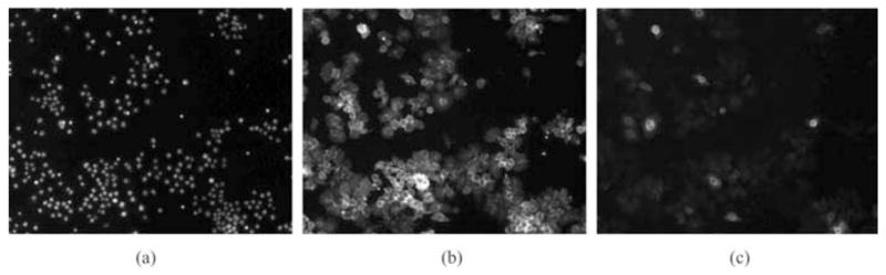
Sample RNAi fluorescent images of three channels. (a) DNA channel, (b) actin channel and (c) Rac channel. Original image of each channel contains 1280 × 1024 pixels.
Since hundreds of thousands of images with rather poor quality are generated in each study, cells from cell-based assays must be segmented automatically in a cost-effective manner. Three phenotypes with distinct shapes are observed, which are namely, round, spiky and ruffled ones. Images are shown in Fig. 2. Accurate segmentations of these cells with specific phenotypes are necessarily needed for further analysis. However, because of the dense clustering and obscure boundaries of cells, existing techniques cannot be directly applied to Actin or Rac channel image to get a satisfactory segmentation.
Fig. 2.
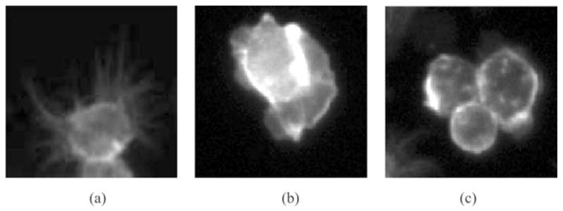
Patches of RNAi cell image in the Actin channel with specific phenotypes. (a) Spiky shape, (b) ruffled shape and (c) round shape.
Comparatively, nuclei in DNA channel are clearly screened, and relatively easy to segment. Extracted nuclei can be used to instruct segmentation of cells in other channels. Simple thresholding algorithms, such as Otsu’s method (Otsu, 1978; Ridler & Calvard, 1978), can easily complete this task by computing a threshold value and setting the pixel whose grey level is higher than the threshold value as foreground. However, there still remain some problems. Sometimes, significant intensity variations exist between close nuclei; thus, a lower threshold value may cause these nuclei to be segmented as a whole, whereas a higher threshold value may help to separate the nuclei, but it may cause some nuclei to be missed or split at the same time. In addition, noise may be regarded as nuclei.
Fortunately, accuracy of nuclei segmentation can be evaluated by the following basic biological information: (1) Only one nucleus exists within each cell and near its centre, which means that one nucleus cannot enter another nucleus’s domain. (2) The shape of nucleus is nearly convex. As a result, a non-convex object will be regarded as under-segmented. (3) With the resolution of image acquisition known, the range of nucleus’s size is estimated empirically. If the size of an object is larger than its range, it should be judged as a case of under-segmentation; if the size of an object is smaller than the range, the object should be considered as noise. (4) Noise is observed to be comparatively bright. If the average intensity of the object is higher than normal range, the object will also be considered as noise. Obviously, any global thresholding algorithm cannot address the above problems. Instead, an adaptive thresholding algorithm in Xiong et al. (2006) is employed: (1) apply Otsu’s method to threshold the DNA channel image and label each extracted object in a candidate list; (2) if one object is regarded as noise according to its intensity or size, it will be removed from the candidate list; (3) if one object is regarded to be under-segmented according to its shape or size, touching nuclei will be separated by adopting a higher threshold value to threshold in its convex hull region; (4) repeat steps (2) and (3) until all extracted objects are regarded as normal nuclei.
With the information of extracted nuclei, cells are segmented in the second step. A novel scale-adaptive steerable filter in the next section is designed to enhance the image in Actin channel and details of cell segmentation are presented in the section on Cell Segmentation.
Spiky cell enhancement using scale-adaptive steerable filter
Cells of ‘spiky’ phenotype in real-RNAi data are observed to have many long and thin protrusions with relatively low intensities. These protrusions cannot be extracted wholly by simple thresholding methods. Here, a novel scale adaptive steerable filter is designed to help solve this problem. Steerable filter theory (Freeman & Adelson, 1991) has been used in many computer vision tasks, such as texture analysis, edge detection and image enhancement. Usually, steerable filter is composed of a class of basic filters, whose impulse response at any arbitrary angle can be synthesized from a linear combination of the same filter’s impulse response rotated to certain directions with a set of prespecified rotation functions as interpolating parameters. For example, let G (x, y) be the filter’s impulse response; the filter’s rotated impulse response at an angle θ, Gθ(x, y), can be written as:
| (1) |
where M is the number of basic filters, Gθj (x, y) is the jth basic filter, θj is the j th basic angle, j ∈ 1, 2, …, M and kj(θ) is the j th interpolating parameter.
In our experiment, steerable filter is designed based on the second derivatives of circularly symmetric Gaussian function G (x, y, σ) given by Freeman and Adelson, (1991).
| (2) |
Three basic angles, θ1 = 0, θ2 = π/4 and θ3 = π/2, are selected to implement the steering property. The steerable filter is designed as follows.
| (3) |
with
| (4) |
| (5) |
| (6) |
where σ determines the scale of the filter, and A(σ) normalizes the integral of |Gxx(x, y, σ)|2 over the R2 plane to unity on the scale σ.
In our approach, enhancement is achieved through angularly adaptive filtering of the image using the steerable filter. Let I (x, y) be the given image, and Wθ(x, y, σ) be the result of filtering I (x, y) with the filter Gθ(x, y, σ) on the certain scale σ. The corresponding squared magnitude |Wθ(x, y, σ)|2 can be computed at any angle θ. At every pixel p(i, j), the dominant orientation direction at which squared magnitude is the largest will be found and its squared magnitude will be taken as the ‘optimal enhanced value’ on that pixel. The enhanced image is taken as W(x, y, σ) called ‘optimal enhanced image’. When applying the steerable filter to real-RNAi images, the scale σ plays an important role in determining the enhancement quality of the long and thin protrusions. Obviously, the steerable filter on a certain scale σ can only enhance the protrusion of certain width. Since protrusions of different widths exist in RNAi images, they should be specially enhanced by the steerable filter on a different scale σ in order to get the best performance. As a result, we propose a scale-adaptive steerable filter to achieve the goal.
During our application, the scale range [σmin, σmax ] (σ ∈ [σmin, σmax ]) is defined as [0.5, 1.1] empirically. Scale is sampled as σi in this range (σi ∈ [σmin, σmax ], σi is the i th sampled scale, i ∈1, 2, …, N, N is the number of sampled scales). The steerable filter Gθ(x, y, σi) on different sampled scale σi convolutes with the original image I (x, y) to get the corresponding ‘optimal enhanced image’ W(x, y, σi). Generally, the larger magnitude value in enhanced image means the better enhancement performance. Therefore, at each pixel p(i, j), the final enhanced value W(i, j) is selected as
| (7) |
where N is the number of sampled scale. Consequently, the best performance is achieved by adaptively choosing steerable filter of certain scale σ to enhance long and thin protrusions of different widths.
In Fig. 3, effects of enhancement on different values of σ are illustrated. Figure 3(a) shows the image enhanced by steerable filter on σ = 0.5. Figure 3(b) shows the image enhanced by steerable filter on σ = 0.9. Figure 3(c) shows the image enhanced by steerable filter on σ = 1.1.
Fig. 3.
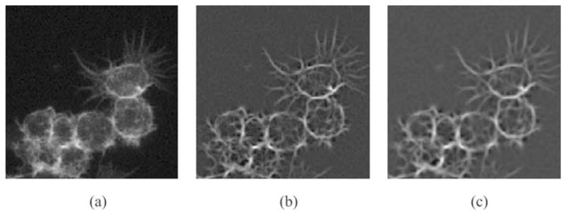
(a) The image enhanced by steerable filter on σ = 0.5. (b) The image enhanced by steerable filter on σ = 0.9. (c) The image enhanced by steerable filter on σ = 1.1.
In Fig. 4, two groups of images are illustrated. Figures 4(a) and (e) show the original image of clustered cells, in which spiky cells exist. The thresholding method is directly applied to Figs 4(a) and (e) and gets the binary segmentation result. The contours of extracted cells are shown in green in Figs 4(b) and (f). Obviously, long and thin protrusions cannot be extracted completely. Therefore, the scale-adaptive steerable filter is applied to Figs 4(a) and (e). Figures 4(c) and (g) show the enhanced image, whereas Figs 4(d) and (h) illustrate the extracted cells based on the information of both original and enhanced images, which segment the long and thin protrusions on RNAi cells completely.
Fig. 4.
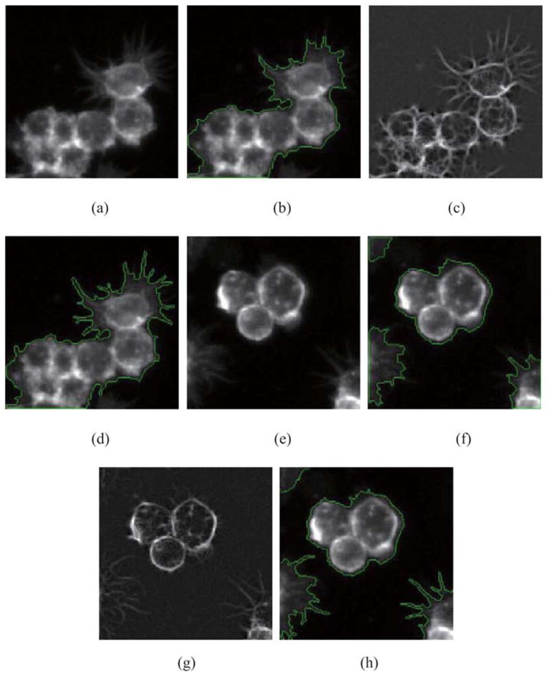
(a) The original image of spiky cells. (b) Extracted cells from the original image. (c) Enhanced image by steerable filter. (d) Extracted cells from the enhanced image. (e) Another original image of cells. (f) Extracted cells from the original image. (g) Enhanced image by steerable filter. (h) Extracted cells from the enhanced image.
Cell segmentation
In this section, we proposed our segmentation method based on constraint factor GCBAC and morphological algorithms, which consists of the following steps. First, based on the nuclei extracted from the DNA channel, we employ region-growing algorithm to find initial contours of cells. Second, constraint factor GCBAC method is presented in the next section to segment RNAi cells using initial contours. Finally, morphological algorithm is combined with constraint factor GCBAC to be an integrated method in the section on Clustered Cells Segmentation to separate tightly clustered cells.
The first step is to find initial contours for constraint factor GCBAC automatically. Generally, only one nucleus exists in one cell and near its centre; therefore, region-growing algorithm (Garbay et al., 1986; Gonzalez & Woods, 2002) can use extracted nuclei as seed regions to find initial contours. The basic approach is to start with a set of points as seed region and group their neighbouring pixels into seed region according to the pre-defined criteria. Here, we define two simple criteria: (1) the grey level of any pixel must be in a specified range around the average grey level of pixels in the seed region. If the average grey level is α, the grey level of grouping-allowed pixel β should satisfy: β ∈ [α − L1, α + L2], where L1 and L2 are the specified range sizes. We will discuss these parameters in the section on Experimental Results and Comparisons. (2) The pixels must be eight-connectivity neighbour of any one pixel in the seed region. Note that the growing regions of nuclei are not allowed to overlap others when several nuclei are growing simultaneously.
In the following, constraint factor GCBAC method and morphological algorithms are developed to extract and separate tightly clustered cells.
Constraint factor GCBAC method
Constraint factor GCBAC method overcomes graph cut method’s well-known shortcoming of yielding short boundaries and active contour method’s well-known shortcoming of local minima, while inheriting the advantage of global optimization and being polynomial time-consuming. s − t min cut, as the basic theory of graph cuts, will be introduced first.
Let G = (V, E) (V is the set of vertices, E is the set of edges between vertices) be an undirected graph with vertices i, j ∈V, and edges of neighbouring vertices (i, j) ∈E. The corresponding edge weight c(i, j) is a nonnegative measurement of the similarity between neighbouring elements i and j. Also, there are two special nodes called terminals, namely, the source s and the sink t. A cut with source s and sink t is defined as a partition of V into two sets: S and T, T = V − S, whereas the cut’s value is the summation of edge weights across the cut.
| (8) |
Consequently, s − t min cut is to find an optimal cut, whose summation of its edge weights is the smallest. The s − t min cut can be computed exactly in polynomial time via algorithms (Ford & Fulkerson, 1962) for two terminal graph cuts. Several polynomial-time algorithms for solving min-cut problem are described in Ahuja et al. (1993)). Experimental comparison of several different min-cut algorithms can be seen in Boykov and Kolmogrov (2004).
In our approach, the image is represented as an adjacency graph. Each pixel is represented as a vertex, and edges only exist between eight-connectivity neighbouring vertices. Neither edges nor edge weights exist between non-neighbouring pixels. Clearly, the edge weight function between vertices plays an important role in determining the accuracy of the following segmentation (Kolmogorov & Zabih, 2004). Traditional definition of edge weight using gradient information of original image is not enough to instruct accurate segmentation, owing to the significant intensity variations inside cells. For example, a cell’s inner part is much brighter than the outer part; such edge weight functions may cause the method to segment the inner part finally.
The concept of constraint factor has been introduced in Xiong et al. (2006) to solve the similar problem. Constraint factor is some kind of binary mask, which encodes global regional information as a supplement to the edge information in gradient of the original image. Motivated by the constraint factor, we incorporate a similar idea into our approach.
Assuming I as the original image, the binary segmentation of the original image I is used as the constraint factor H (I). The classical Otsu’s method considers the segmentation as a problem of two-class clustering. However, this assumption is often not true when dealing with fluorescence RNAi images. Generally, the threshold value of classical Otsu’s method is relatively high; as a result, only bright part inside cells is segmented. Instead, a modified Otsu’s method is employed. The image is logarithmic-transformed first; then, classical Otsu’s method is applied to the transformed image to get its threshold value; finally, this threshold value is exponential transformed and the value obtained is used to threshold the original image. In Fig. 5, three images are illustrated. Figure 5(a) shows the original image. Figure 5(b) shows the result of classical Otsu’s method. Obviously, existing holes inside the extracted cytoplasm cause a poor result. Comparatively, the result of the modified Otsu’s method in Fig. 5(c) is much more accurate.
Fig. 5.
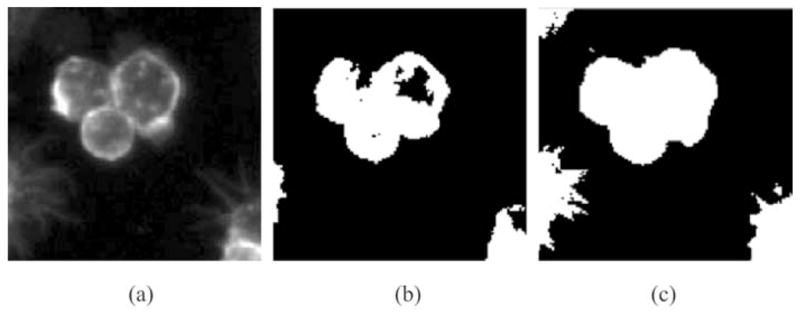
Results of both classical Otsu’s method and the modified Otsu’s method. (a) The original image. (b) Cytoplasm segmentation of Otsu’s algorithm. (c) Cytoplasm segmentation of the modified Otsu’s algorithm.
After the constraint factor H (I) is obtained, pixels’ grey level in both original image I and constraint factor H (I) are normalized to [0, 255]. Then, constraint factor image N(I) is computed by incorporating the constraint factor as follows:
| (9) |
Constant λ (0 < λ < 1) is a scalar parameter that weights the importance of two sources of information. If λ is large, we trust more original information; otherwise, we trust more global information from H (I). In our experiment, λ is selected as 0.5, which means that both sources of information have the same importance. Therefore, the edge weight function c(i, j) between pixel i and pixel j (pixel i and pixel j must be eight-connectivity neighbours) is designed as follows:
| (10) |
where g(i, j) = exp (− gradij(i)/maxk (gradij(k))) and gradij(k) is constraint factor image N(I)’s pixel intensity gradient at location k in the direction of i → j, n ∈ N. The purpose of the function c(i, j) is to measure the similarity between the pixels: the higher the edge weight, the more similar they are.
After the constraint factor image N(I) is represented as an adjacency graph G, the objective is to find an optimal cut [The objective function is the same as cut(S, T) defined in (8)], which partitions the image into two parts: S and T, and the contours between S and T are regarded as the contours of desired objects. For computation efficiency, depending on initial contour obtained in the region-growing step, constraint factor GCBAC finds the s − t min cut within the contour’s neighbourhood to extract the corresponding RNAi cell, and the optimal solution is obtained using excess scaling pre-flow push algorithm(Ahuja et al., 1993). To that end, we summarize the framework of constraint factor GCBAC as follows (Xu et al., 2003):
Given an initial contour, dilate current contour into its contour’s neighbourhood with an inner boundary and an outer boundary (Fig. 6).
Identify all the vertices corresponding to the inner boundary and outer boundary as a single source s and a single sink t.
Compute the s − t min cut to obtain a new boundary that better separates the inner boundary from the outer boundary.
Return to step 1 until the algorithm converges.
Fig. 6.
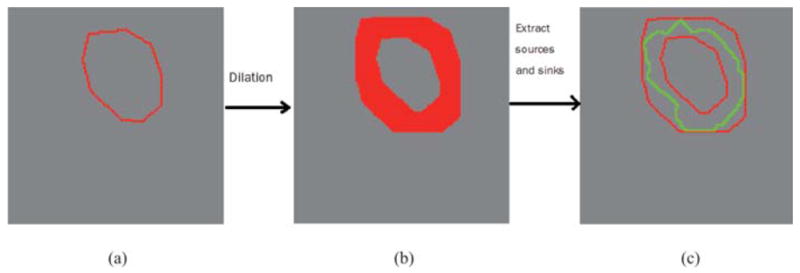
Process of finding optimal solution. (a) Initial contour shown in red. (b) Dilation of the initial contour. (c) Optimal contour shown in green.
Example figures are shown in Fig. 6 to explain each step of constraint factor GCBAC. Figure 6(a) illustrates an initial contour in red. Then, the neighbouring region of the initial contour is obtained through dilation, which is shown as a red narrow band in Fig. 6(b). Finally, the s − t min cut is computed to separate the narrow band into two parts, and the touching boundary of two parts is shown in green in Fig. 6(c) as the segmentation result.
Our constraint factor GCBAC is able to handle RNAi cells, in which intensity variations exist. Figure 7 shows a group of results. Figures 7(a) and (b) show the original image I and constraint factor image N(I), where λ = 0.5. Clearly, intensity contrast between cytoplasm and background in constraint factor image N(I) is much larger than that in original image I; as a result, constraint factor GCBAC will be able to segment the whole RNAi cell than just the bright inner part. In Fig. 7(c), GCBAC without constraint factor only segments the bright parts inside the cell. In Fig. 7(d), our constraint factor GCBAC segments the whole cell from the background.
Fig. 7.
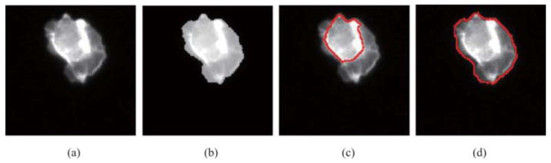
Segmentation results of both traditional GCBAC and constraint factor GCBAC. (a) Original image I of an RNAi cell. (b) The constraint factor image N(I). (c) Segmentation result without constraint factor. (d) Segmentation result using constraint factor.
Clustered cells segmentation using constraint factor GCBAC and morphological algorithm
Constraint factor GCBAC is designed in the section on Constraint factor GCBAC Method to segment RNAi cells in Actin channel. First, Constraint factor GCBAC uses the boundary of constraint factor H (I) as the initial contour to extract the whole cytoplasm of clustered cells. Then, the initial contour for each nucleus has been found by region-growing algorithm, and constraint factor GCBAC method uses each initial contour to segment the corresponding cell. However, since clustered cells touch closely and weak or even no edges exist in the touching region, cell segmentation is not always satisfactory. Boundaries of segmented cells cannot touch others closely. When two adjacent cells are segmented by the constraint factor GCBAC, the relationship of their boundary positions has three possible cases generally: (1) Part of one cell’s boundary touch the other closely. This case is regarded as the satisfactory case. (2) Segmented cells are partly overlapped and their boundaries intersect. (3) Part of both cells’ boundaries is repulsive, leaving blank regions between segmented cells. In our experiments, the touching boundaries in case 1, overlapped regions in case 2 and repulsive regions in case 3 can all be regarded as touching regions between tightly clustered cells.
The touching regions must be extracted according to the following criteria. (1) The pixel must belong to the area of clustered cells’ cytoplasm first. (2) If a pixel belongs to the area of clustered cells’ cytoplasm, while it belongs to none of the areas of segmented cells, the pixel will be regarded to be of the repulsive regions. (3) If a pixel belongs to the area of clustered cells’ cytoplasm, although it belongs to the areas of several segmented cells, the pixel will be regarded to be overlapped regions. (4) If a pixel belongs to the area of clustered cells’ cytoplasm, while the pixel satisfies: the pixel belongs to the area of one segmented cell, and parts of its eight-connectivity neighbouring pixels belong to the areas of other segmented cells. This pixel will be regarded to be touching regions.
In Fig. 8, we use artificial images to illustrate three possible cases and the corresponding touching regions. In Fig. 8(a), two cells are clustered with no edges existing in their touching regions. Owing to weak or even no edges existing in touching regions, the touching cytoplasm is segmented as a whole. The black contour shows the boundary of touching cells. Two nuclei are marked blue and red in the cells. Then, constraint factor GCBAC uses the information of nuclei to implement cell segmentation. The boundaries of two segmented cells are shown in blue and red, respectively. Three possible cases may exist generally. In Fig. 8(b), segmented cells are overlapped. The overlapped region, which is shown in blue, is regarded as the touching region. In Fig. 8(c), the two segmented cells touch closely. Then, their touching edges, including the blue edge and red edge, will be taken as the touching region. In Fig. 8(d), the boundaries of two segmented cells are repulsive. The region in yellow between the segmented cells is also taken as the touching region.
Fig. 8.
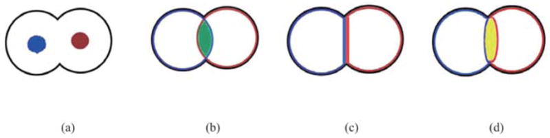
Three possible cases of touching regions. (a) Nuclei and their touching cytoplasm. (b) Overlapped case. (c) Touching case. (d) Repulsive case.
After the touching regions have been extracted, the boundary of the whole cytoplasm obtained by constraint factor GCBAC is extracted and integrated with the touching regions to be a whole called ‘boundary-incorporated-touching regions’. Finally, mathematical morphological thinning algorithm (Gonzalez & Woods, 2002) is applied to the boundary-incorporated-touching regions iteratively. Since the boundary of the cytoplasm is 1 pixel in width, it will keep unchanged, while touching edges between dense clustered cells can be extracted by thinning touching regions. When touching edges are of 1 pixel width, morphological thinning algorithm stops. The thinning result is regarded as the final segmentation result. The segmentation result seems very good. In the next section, we apply our approach to real-RNAi drosophila images. The whole process of segmentation and final segmentation results will be illustrated.
Experimental results and comparisons
In this section, we apply the proposed approach to real-RNAi data sets, especially three distinct shapes: round, spiky and ruffled, and get experimental results on segmentation of Drosophila RNAi images. Since automated segmentation is required and each image contains different kinds of cells, the fixed universal parameters are needed. We tried out all the parameters settings within a specified range on an image and the parameter setting with the best performance is then used for segmentation of all the images. The values of the parameters in our experiments are shown in Table 1. [amin, amax] are the area ranges for judging normal nucleus. [σmin, σmax] are the sampled scale ranges in scale-adaptive steerable filter. L1, L2 are the range sizes of grey scale used in region-growing algorithm. n is the power value in Eq. (10), which is used to penalize the similarity between vertices. λ (0< λ < 1)is a scalar parameter to weight the importance of the two sources of information in constraint factor GCBAC. In the following, the segmentation process of our method will be illustrated first. Then, performances of our approach and other methods are compared and evaluated.
Table 1.
Parameters settings in the experiment.
| Parameter | amin | amax | σmin | σmax | L1 | L2 | λ | n |
|---|---|---|---|---|---|---|---|---|
| Value | 120 | 500 | 0.5 | 1.1 | 40 | 30 | 0.5 | 6 |
Clustered cells segmentation using constraint factor GCBAC and morphological algorithms
Figure 9 demonstrates the whole process of clustered cells segmentation using our approach. Figures 9(a) and (b) show the original images of cytoplasm in the Actin channel and nuclei in the DNA channel, respectively. Figure 9(c) shows the result of cytoplasm segmentation in the Actin channel. The red boundary segments the cytoplasm of clustered cells as a whole. The nuclei in the DNA channel are segmented by our adaptive thresholding algorithm. In Fig. 9(d), extracted nuclei are shown by red boundaries in cytoplasm. Then, region-growing algorithm finds initial contours for extracted nuclei. In Fig. 9(e), initial contours for nuclei are shown in red. The constraint factor GCBAC uses initial contours to segment clustered cells, respectively. In Fig. 9(f), segmented cells are shown in red boundaries. Because of the significant intensity variations inside clustered cells, segmented cells cannot touch others closely. Segmented cells may touch, repulse or overlap. In Fig. 9(g), segmented cells are shown in grey. The white areas are overlapped areas. The black areas between cells are repulsive areas. These regions are called ‘touching regions’, which are extracted and shown in Fig. 9(h). Then, the boundary of cytoplasm is incorporated into touching regions, which is called ‘boundary-incorporated touching regions’, is shown in Fig. 9(i). Morphological thinning algorithm is applied to the boundary incorporated touching regions iteratively and extracts skeleton. The result is shown in Fig. 9(j). This result could be regarded as final segmentation result. In Fig. 9(k), the final segmentation result is demonstrated using red contours.
Fig. 9.
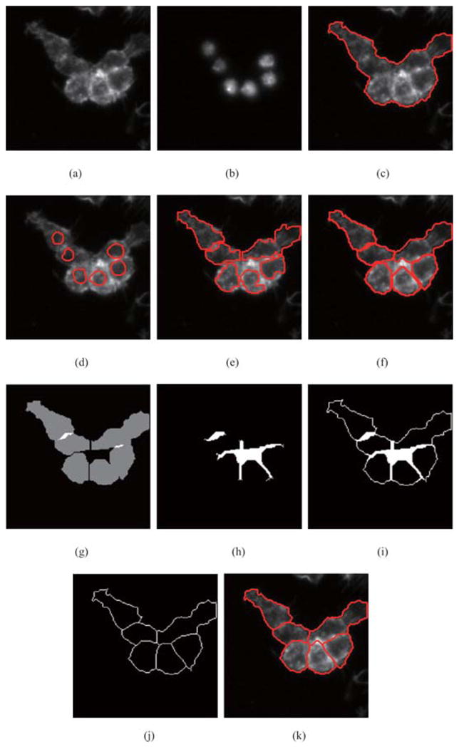
The process of clustered cells segmentation. (a) Original image of cytoplasm. (b) Original image of nuclei. (c) Cytoplasm segmentation by constraint factor GCBAC. (d) Extracted nuclei in cytoplasm. (e) Initial contour of nuclei found by region-growing algorithm. (f) Cell segmentation results by constraint factor GCBAC. (g) Segmented cells are shown in grey. (h) Extracted touching regions. (i) Boundary-incorporated regions. (j) Result of morphological thinning algorithm. (k) Final segmentation result.
Comparisons of our segmentation of clustered cells with that of seeded watershed
Some image patches are randomly obtained, in which three main distinct shapes, round, ruffled and spiky, are contained. We apply the proposed approach to these images, and the corresponding segmentation results are demonstrated in Figs 8 and 9 to prove the effect of our algorithm. For comparison purpose, we also depend on the widely used open source software CellProfiler (Carpenter et al., 2006) with default parameter setting to implement seeded watershed method on the same data set and get corresponding segmentation results. The performances of our method and seeded watershed are then compared.
In Fig. 10, spiky cells are contained. Figures 10(a) and (b) show the original images of nuclei in DNA channel and cytoplasm in Actin channel. Nuclei are extracted and shown by red boundaries in Fig. 10(c). Our approach uses the information of extracted nuclei to instruct clustered cells segmentation. The result is shown in Fig. 10(d). For comparison, seeded watershed method is applied to Figs 10(a) and (b), and the segmentation result is shown in Fig. 10(e). For evaluation, manual segmentation of biologist is obtained as ground truth, which is shown in Fig. 10(f). CellProfiler is not able to get specific shapes existing in RNAi data sets. Comparatively, our approach’s result looks better than seeded watershed’s result.
Fig. 10.
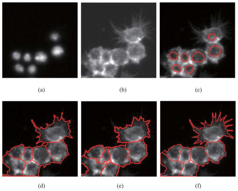
Comparison of segmentation performance between our approach and seeded watershed. (a) Nuclei in DNA channel (b) Cytoplasm in Actin channel. (c) Extracted nuclei in Actin channel. (d) Result of our approach. (e) Result of seeded watershed method. (f) Ground truth obtained by manual segmentation.
In the following Fig. 11, ruffled cells are contained. Both our approach and seeded watershed method are applied to the same data and their results are compared. Note that CellProfiler cannot distinguish between noise and real nucleus; as a result, noise is wrongly segmented as nucleus, which causes inaccurate results. In Fig. 11(e), extracted objects with red contours are selected to instruct cytoplasm segmentation. Obviously, noise is regarded as a nucleus. CellProfiler tends to lead over-segmentation of the cells. Corresponding results are shown in Fig. 11(f). Our approach has the ability to distinguish noise and nucleus. Our results are shown in Fig. 11(d), and the ground truth is shown in Fig. 11(g).
Fig. 11.
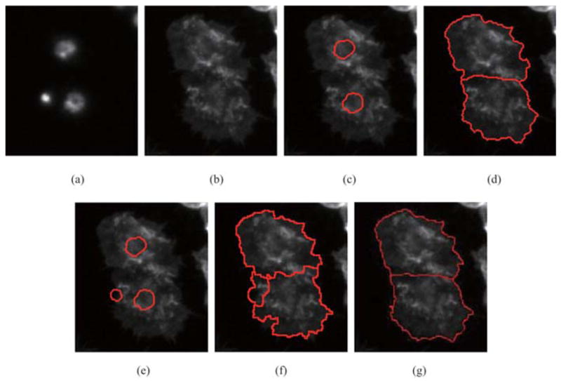
Comparison of segmentation performance between our approach and seeded watershed. (a) Nuclei in DNA channel (b) Cytoplasm in Actin channel. (c) Extracted nuclei using our approach. (d) Result of our approach. (e) Extracted nuclei using CellProfiler software. (f) Result of CellProfiler. (g) Ground truth obtained by manual segmentation.
Comparisons between our approach and geodesic active contour method
As we note in the previous section, another kind of popular segmentation technique is based on active contour. Xiong et al. (2006) used geodesic active contour–based method and level sets algorithm to solve the problem of RNAi image segmentation. The experiment results look excellent in his paper. However, geodesic active contour method has the disadvantage of being unreasonably time-consuming. Compared with geodesic active contour methods, our approach has the advantage of being polynomial time-consuming. Here, we apply our method and Xiong’s method to the same image patches on the same laptop with Centrino 1.6 GHz CPU and 768 MB memory. Processing times of the two methods are displayed in Table 2; it is obvious to see that our method consumes much less time than Xiong’s method. Also, the performances of our method and that of Xiong’s method are illustrated in Fig. 12. Figure 12(a) shows nuclei in the DNA channel. In Fig. 12(b), clustered cells cannot be segmented satisfactorily. Boundaries of extracted cells cannot touch with others.
Table 2.
Comparisons of processing times.
| Our method | Xiong’s method | |
|---|---|---|
| Patch 1 | 27 s | 1580 s |
| Patch 2 | 27 s | 1551 s |
| Patch 3 | 33 s | 1733 s |
Fig. 12.
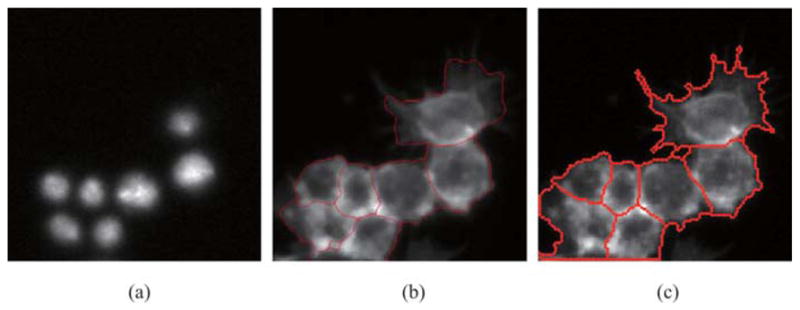
Comparison of segmentation performance between our approach and geodesic active contour method. (a) Nuclei in DNA channel. (b) Segmentation result of geodesic active contour method. (c) Segmentation result of our approach.
Quantitative evaluation
Quantitative performance evaluation is performed by comparing our results with the ground truth. For comparison purpose, the segmentation results of seeded watershed method implemented by CellProfiler and geodesic active contour method implemented by Xiong’s program (Xiong et al., 2006) on our data sets are also provided. The performance of our method and those of the seeded watershed method and geodesic active contour method has been illustrated and compared previously.
Our approach outperforms the CellProfiler in three ways. The first problem is that the CellProfiler sometimes fails to discard noise, which leads to the over-segmentation of the cells. The second problem is that CellProfiler is not able to get the specific cell shapes existing in our data sets. Comparatively, our approach could segment the whole spiky shape. The final problem is that the accuracy of clustered cells segmentation obtained by our approach is often higher than that of CellProfiler.
Our approach outperforms the geodesic active contour in two ways. One aspect is about the processing time. Our approach consumes much less time than Xiong’s method. The other aspect is that Xiong’s method sometimes fails to tackle tightly clustered cells where large intensity variations exist. As we illustrate in the section on Comparisons between Our Approach and Geodesic Active Contour Method, the whole cell cannot be extracted, or extracted cells cannot touch with others perfectly. Comparatively, our method is able to get better segmentation results.
In order to analyze the accuracy of the proposed approach, the F-score is employed as our performance measure. F-score is an evaluation measure computed from the precision and the recall values that are standard techniques used to evaluate the quality of the results of a system against the ground truth. Let X denotes the segmented regions of automatic segmentation result and Y is segmented regions of the ground truth, which is manual segmentation by biologists. The precision p and recall r are given by
| (11) |
The F-score is computed by taking the harmonic average of the precision and the recall:
| (12) |
The F-score is then computed by taking the harmonic average of the precision and the recall (van Rijsbergen, 1979), where β is the weighting parameter. In order to give the equal weight to precision and recall, a common approach is to set β = 1, such that F1 = 2pr/(p + r).
In Fig. 13, F1-scores of our method, the CellProfiler and level sets method (Xiong et al., 2006) are shown. When computing the scores, 12 sets of images are randomly chosen from all the data sets. Manual segmentation results on these images are obtained as ground truth. Compared with seeded watershed method, F1-scores of our approach are higher on most image sets. This can be explained by the reasons that the CellProfiler may have high precision values but the recall values are pretty low, whereas our method may have both high precision and high recall values. Compared with level sets method (Xiong et al., 2006), F1-scores of our approach are much higher on some image sets, owing to the fact that some cells cannot be segmented completely by level sets method, such as the examples in Fig. 12(b). However, F1-scores of level sets method are higher than those of our approach and seeded watershed method on some other image sets, which means that level sets method still has the advantage of accurate segmentation, even though it is highly time-consuming.
Fig. 13.
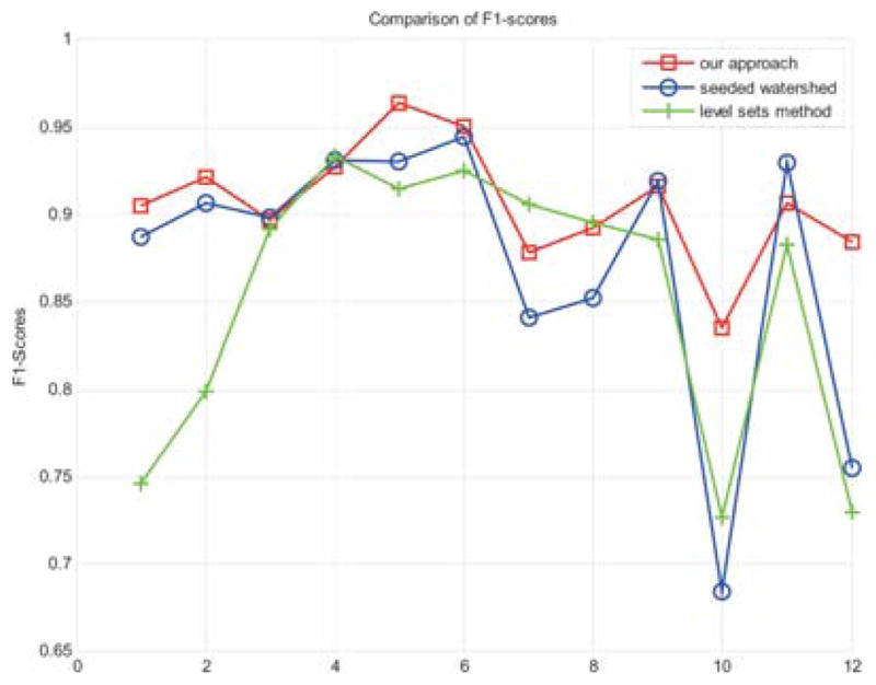
The F1-score of our method and the CellProfiler.
Conclusion and discussion
In this paper, we present a new approach for automatic segmentation of RNAi fluorescent cellular images. The proposed approach consists of two steps: nuclei segmentation and cytoplasm segmentation. In the first step, nuclei are extracted. Labelled nuclei are initialized to instruct the latter segmentation. In the second step, in order to extract long and thin protrusions on the spiky cells, a novel scale-adaptive steerable filter is designed to enhance the image first. Then, constraint factor GCBAC method and morphological algorithms are combined to segment tightly clustered cells. Promising experimental segmentation results on RNAi fluorescent cellular images are presented. Compared with other segmentation techniques, our novel approach has advantages of automatically segmenting RNAi cells in polynomial time. Excellent experimental results verify the effectiveness of our proposed approach. Our future work is to extend the segmentation to high-throughput imaging RNAi experiments of other cell types.
Acknowledgments
The authors would like to acknowledge the assistance of their biology collaborators in the Department of Genetics at Harvard Medical School in this research effort. The funding support of Drs Zhou and Wong is from HCNR Center for Bioinformatics Research Program and the NIH R01 LM008696.
References
- Ahuja N, Magnanti T, Orlin J. Network Flows: Theory, Algorithms and Applications. Prentice Hall; New Jersey: 1993. [Google Scholar]
- Bamford P, Lovell B. Unsupervised cell nucleus segmentation with active contours—an efficient algorithm based on immersion simulations. Signal Process. 1998;71:203–213. [Google Scholar]
- Blake A, Rother C, Brown M, Perez P, Torr P. Interactive image segmentation using an adaptive GMMRF model. Eur Conf Comput Vis. 2004;3:428–441. [Google Scholar]
- Boutros M, Kiger AA, Armknecht S, et al. Genome-wide RNAi analysis of growth and viability in drosophila cells. Science. 2004;303:832–835. doi: 10.1126/science.1091266. [DOI] [PubMed] [Google Scholar]
- Boykov Y, Funka-Lea G. Graph cuts and efficient N-D image segmentation. Int J Comput Vis. 2006;70(2):109–131. [Google Scholar]
- Boykov Y, Jolly M. Interactive graph cuts for optimal boundary and region segmentation of objects in N-D images. Int Conf Comput Vis. 2001;1:105–112. [Google Scholar]
- Boykov Y, Kolmogorov V. Computing geodesic and minimal surfaces via graph cuts. Int Conf Comput Vis. 2003;1:26–33. [Google Scholar]
- Boykov Y, Kolmogorov V. An experimental comparison of min-cut/max-flow algorithms for energy minimization in vision. IEEE Trans Pattern Anal Mach Intell. 2004;26(9):1124–1137. doi: 10.1109/TPAMI.2004.60. [DOI] [PubMed] [Google Scholar]
- Boykov Y, Kolmogorov V, Cremeers D, Delong A. An integral solution to surface evolution PDEs via geo-cuts. Eur Conf Comput Vis. 2006;3:409–422. [Google Scholar]
- Carpenter A, Jones T, Lamprecht M, et al. CellProfiler: image analysis for high throughput microscopy. 2006 Available at URL: http://www.Cellprofiler.org.
- Caselles V, Kimmel R, Sapiro G. Geodesic active contours. Int J Comput Vis. 1997;22(1):61–79. [Google Scholar]
- Chen S, Cao L, Liu J, Tang X. Automatic segmentation of lung fields from radiographic images of SARS patients using a new graph cuts algorithm. Int Conf Pattern Recognit. 2006;1:271–274. [Google Scholar]
- Dufour A, Shinin V, Tajbakhsh S, Guillén-Aghion N, Olivo-Marlin JC, Zimmer C. Segmentation and tracking fluorescent cells in dynamic 3-D microscopy with coupled active surfaces. IEEE Trans Image Process. 2005;14(9):1396–1410. doi: 10.1109/tip.2005.852790. [DOI] [PubMed] [Google Scholar]
- Ford L, Fulkerson D. Flows in Networks. Princeton University Press; New Jersey: 1962. [Google Scholar]
- Freeman W, Adelson E. The design and use of steerable Filters. IEEE Trans Pattern Anal Mach Intell. 1991;13(9):891–906. [Google Scholar]
- Garbay C, Chassery JM, Brugal G. An iterative region-growing process for cell image segmentation based on local color similarity and global shape criteria. Anal Quant Cytol Histol. 1986;8:25–34. [PubMed] [Google Scholar]
- Garrido A, Pérez de la Blanca N. Applying deformable templates for cell image segmentation. Pattern Recogn. 2000;33(5):821–832. [Google Scholar]
- Gonzalez RC, Woods RE. Digital Image Processing. 2. Prentice Hall; New Jersey: 2002. [Google Scholar]
- Kiger A, Baum B, Jones S, Jones M, Coulson A, Echeverri C, Perrimon N. A functional genome analysis of cell morphology using RNA interference. J Biol. 2003;2:27. doi: 10.1186/1475-4924-2-27. [DOI] [PMC free article] [PubMed] [Google Scholar]
- Kass M, Witkin A, Terzopoulos D. Snakes: active contour models. Int J Comput Vis. 1987;1:321–331. [Google Scholar]
- Kolmogorov Y, Boykov Y. What metrics can be approximated by geo-cuts, or global optimization of length/area and flux. International Conference on Computer Vision. 2005;1:564–571. [Google Scholar]
- Kolmogorov Y, Zabih R. What energy functions can be minimized via graph cuts. IEEE Trans Pattern Anal Mach Intell. 2004;26(2):147–159. doi: 10.1109/TPAMI.2004.1262177. [DOI] [PubMed] [Google Scholar]
- Kumar M, Torr PHS, Zisserman A. OBJ CUT. IEEE Conference of Computer Vision and Pattern Recognition. 2005;1:18–25. [Google Scholar]
- Malpica N, Ortiz de Solórzano C, Vaquero JJ, Santos A, Vallcorba I, García-Sagredo JM, del Pozo F. Applying watershed algorithms to the segmentation of clustered nuclei. Cytometry. 1997;28:289–297. doi: 10.1002/(sici)1097-0320(19970801)28:4<289::aid-cyto3>3.0.co;2-7. [DOI] [PubMed] [Google Scholar]
- Otsu N. A threshold selection method from gray level histogram. IEEE Trans Syst Man Cybern. 1978;8:62–66. [Google Scholar]
- Osher S, Sethian JA. Fronts propagating with curvature-dependent speed: algorithms based on Hamilton-Jacobi formulations. J Comp Phy. 1988;79:12–49. [Google Scholar]
- Ortiz de Solórzano C, Malladi R, Lelievre SA, Lockett SJ. Segmentation of nuclei and cells using membrane related protein markers. J Microsc. 2001;201:404–415. doi: 10.1046/j.1365-2818.2001.00854.x. [DOI] [PubMed] [Google Scholar]
- Ridler TW, Calvard S. Picture thresholding using an iterative selection method. IEEE Trans Syst Man Cybern. 1978;8:62–66. [Google Scholar]
- Sethian J. Level Set Methods and Fast Marching Methods. 2. Cambridge University Press; Cambridge: 1999. [Google Scholar]
- Shi J, Malik J. Normalized cuts and image segmentation. IEEE Trans Pattern Anal Mach Intell. 2000;22(8):888–905. [Google Scholar]
- Slabaugh G, Unal G. Graph cuts segmentation using an elliptical shape prior. IEEE Int. Conf. Image Processing; 2005. pp. II-1222–II-1225. [Google Scholar]
- van Rijsbergen C. Information Retrieval. 2. Butterworth; 1979. [Google Scholar]
- Vese LA, Chan TF. A multiphase level set framework for image segmentation using the Mumford and Shah model. Int J Comput Vis. 2002;50 (3):271–293. [Google Scholar]
- Vincent L, Soille P. Watersheds in digital spaces: an efficient algorithm based on immersion simulations. IEEE Trans Pattern Anal Mach Intell. 1991;13:583–598. [Google Scholar]
- Wang S, Siskind J. Image segmentation with minimum mean cut. Int Conf Comput Vis. 2001:577–524. [Google Scholar]
- Wählby C, Lindblad J, Vondrus M, Bengtsson E, Björkesten L. Algorithms for cytoplasm segmentation of fluorescence labeled cells. Anal Cell Pathol. 2002;24:101–111. doi: 10.1155/2002/821782. [DOI] [PMC free article] [PubMed] [Google Scholar]
- Wählby C, Sintorn IM, Erlandsson F, Borgefors G, Bengtsson E. Combining intensity, edge and shape information for 2D and 3D segmentation of cell nuclei in tissue sections. J Microsc. 2004;215:67–76. doi: 10.1111/j.0022-2720.2004.01338.x. [DOI] [PubMed] [Google Scholar]
- Wu Z, Leahy R. An optimal graph theoretic approach to data clustering: theory and its application to image segmentation. IEEE Trans Pattern Anal Mach Intell. 1993;15(11):1101–1113. [Google Scholar]
- Xu N, Bansal R, Ahuja N. Object segmentation using graph cuts based active contours. IEEE Conf Comput Vis Pattern Recognit. 2003;2:46–53. [Google Scholar]
- Xiong G, Zhou X, Ji L. Segmentation of drosophila RNAi fluorescence images using level sets. IEEE Trans Circuits Syst I: Fundam Theory Appl. 2006;53(11):2415–2424. [Google Scholar]
- Yang X, Li H, Zhou X. Nuclei segmentation using marker-controlled watershed, tracking using mean-shift, and Kalman filter in time-lapse microscopy. IEEE Trans Circuits Syst I: Regul Pap. 2006;53(11):2405–2414. [Google Scholar]
- Zhao HK, Chan TF, Merriman B, Osher S. A variational level set approach to multiphase motion. J Comp Phy. 1996;127:179–195. [Google Scholar]
- Zhou X, Liu K-Y, Bradley P, Perrimon N, Wong STC. Towards automated cellular image segmentation for RNAi genome-wide screening. Proc Med Image Comput Comput Assist Interv. 2005:885–892. doi: 10.1007/11566465_109. [DOI] [PubMed] [Google Scholar]
- Zhou X, Wong S. High content cellular imaging for drug development. IEEE Signal Process Mag. 2006a;23(2):170–174. [Google Scholar]
- Zhou X, Wong S. Informatics challenges of high-throughput microscopy. IEEE Signal Process Mag. 2006b;23(3):63–72. [Google Scholar]