The emerging discipline of Computational Functional Anatomy

Abstract

Computational Functional Anatomy (CFA) is the study of functional and physiological response variables in anatomical coordinates. For this we focus on two things: (i) the construction of bijections (via diffeomorphisms) between the coordinatized manifolds of human anatomy, and (ii) the transfer (group action and parallel transport) of functional information into anatomical atlases via these bijections. We review advances in the unification of the bijective comparison of anatomical submanifolds via point-sets including points, curves and surface triangulations as well as dense imagery. We examine the transfer via these bijections of functional response variables into anatomical coordinates via group action on scalars and matrices in DTI as well as parallel transport of metric information across multiple templates which preserves the inner product.

Introduction to Computational Functional Anatomy

Advances in the development of digital imaging modalities combined with advances in digital computation are enabling researchers to investigate the precise study of the awesome biological variability of human anatomy. This is the emergent field of computational anatomy (CA) (Grenander and Miller, 1998; Thompson et al., 2004). CA, has three principal aspects: (a) automated construction of anatomical manifolds $M\subset {\mathbb{R}}^3$, points, curves, surfaces, and subvolumes; (b) comparison of these manifolds; and (c) the statistical codification of the variability of anatomy via probability measures allowing for inference and hypothesis testing of disease states.

The automated construction of anatomical manifolds is receiving tremendous focus by many of the groups throughout the world supporting neuromorphometric analyses which are becoming available with large numbers of anatomical samples. Deformable and active models are being used in generating 1-dimensional manifold curves in 2,3 dimensions (Thirion and Goudon,1996; Feldmar et al.,1997; Khaneja et al.,1998; Bartesaghi and Sapiro, 2001;Montagnat et al., 2001, Lorigo et al., 2001; Rettmann et al., 2002; Cachia et al., 2003). The differential and curvature characteristics of curves and surfaces have been examined as well with active and deformable surface models for the neocortex and cardiac systems (Montagnat et al., 2001; Dale and Sereno, 1993; Joshi et al., 1997; Dale et al., 1999; Fischl et al., 1999; Xu et al., 1999; Pham et al., 2000). Local coordinate representations for cortical manifolds have included both spherical and planar representations for studying the brain (Dale and Sereno, 1993; Dale et al., 1999; Fischl et al., 1999; van Essen et al.,1998; Wandell,1999; Bakircioglu et al.,1999; van Essen et al., 2001; Gu et al., 2004; Hurdal and Stephenson, 2004; van Essen, 2004; Mangin et al., 2004; Wang et al., 2005; van Essen, 2005). A great deal of effort has focused on methods of segmentation of anatomical volumes into 3-dimensional submanifolds. Automatic methods for maximum-likelihood and Bayesian segmentation are being developed across the whole brain as well as focus on particular gyri (Wells et al., 1996; Teo et al., 1997; Crespo-Facorro et al., 2000; Shattuck et al., 2001; Fischl et al., 2002; Han et al., 2002; Ratnanather et al., 2003; Dumoulin et al., 2003; Fischl et al., 2004).

There has also been great emphasis for studying anatomical shape variability via vector comparison. The earliest vector mapping of biological coordinates via landmarks and dense imagery was pioneered in the early 1980s and continues today by Bookstein (1978; 1991; 1996) and Bajcsy et al. (1983), Bajcsy and Kovacic (1989), Dann et al. (1989), Gee and Haynor (1999), Gee (1999), and Avants and Gee (2004). Comparison via vector maps based on dense imagery is being carried on with vector mappings restricted to the cortical manifold are being computed as well (Feldmar et al., 1997; Evans et al., 1991; Toga et al., 1991; Collins et al., 1994; Friston et al., 1995; Davatzikos, 1996; Iosifescu et al., 1997; Thompson and Toga, 1999; Warfield et al., 1999; Ashburner, 2007).

Our own contribution in CA has largely focused on large deformation diffeomorphisms as a method for constructing bijective correspondences between anatomical coordinate systems. They are generated by flows as originally proposed (Christensen et al., 1996), which are not additive and provide guaranteed bijections between anatomical configurations. This framework has been formulated as a complete metric space (Grenander and Miller, 1998; Dupuis et al., 1998, Trouvé, 1995a,b, Joshi and Miller, 2000, Miller and Younes, 2001, Miller et al., 2002, Glaunès et al., 2004), providing the mapping methodology with a least-energy (shortest path) and symmetry property.

Currently, the principal focus in the generalized area of the medical image analysis is the study of function as well as structure in the local anatomical coordinates. We refer to this as Computational Functional Anatomy (CFA), which is the extension of the field of CA in the sense that CFA is the mathematical study of anatomical configurations and signals associated with structure and function in anatomical coordinates. The localized manifolds in anatomy are curved coordinate system resulting from the dense packing and interconnection of structures in the body and their functional interrelationship. There is no better illustration of this than in the deep nuclei as well as cortical areas of the brain with its many interconnections. The local curved coordinate systems are evolutionarily stable, and uniquely defined by the micro and macrostructural properties as well as functional properties. Regions of the human body are named and locally defined because of their functional and structural specificity. There are fundamentally two challenges in trying to understand function in anatomical coordinates: (i) signal processing such as filtering, smoothing, interpolation on curved manifolds is simply not as obvious as it is in Euclidean spaces, and (ii) all anatomical structures are different in shape, and therefore local analysis which accommodates statistical variation in populations of individuals is a significant challenge. Therefore, CFA must handle these issues.

This article reviews several of the basic methods in CFA. The first half begins by focusing on the construction of bijective correspondences between anatomical coordinates; both point-set LDDMM as well as dense image methods are presented. The random orbit model is presented, including dense image template estimation. The second half focuses on the transfer of physiological and functional response variables. In particular we show the transfer of fMRI response, cortical thickness, and myelination and track direction as measured in diffusion tensor imagery (DTI). Then we examine the transfer of metric information via parallel transport that preserves the inner product information from one template coordinate system to another. The approach taken here is to define for each anatomical manifold the functional signals F∈F, with $\mathbf{F}\left(x\right),x\in X\subset {\mathbb{R}}^d$. To study populations of functional response in atlas space the bijections g: X↔X^atlas are used to carry or transfer the functional measures according to g: F↦g·F defined through group actions and parallel transport.

The metric shape space

We consider a shape as a generalized image (in the sense of Grenander) indexed over the background space $X\subset {\mathbb{R}}^3$ as an element in the metric shape space I ∈I. This space is constructed as an orbit I =G· I_α of exemplars or templates I_α under groups of transformations G, the groups transforming the objects. The images I ∈I are of two types: (i) point-sets corresponding to landmarks, curves, surfaces, and segmented sub-volumes, and (ii) images corresponding to dense imagery or vectors or tensors, I (x), x∈X. The basic model is that the metric space is a collection of orbits under the transformations of the exemplar templates I=∪_αG·I_α. Flows are used to generate the diffeomorphisms, which connects CA directly to classical mechanics.

The approach constructs the diffeomorphisms g∈G as a flow of ordinary differential equations (ODEs) (Christensen et al., 1996), with g_t, t∈[0, 1] controlled by the Lagrangian evolution according to

$$\frac{\partial g_t}{\partial t}\left(x\right)={\mathit{v}}_t\left(g_t\left(x\right)\right),g_0\left(x\right)=x,x\in X,t\in [0,1].$$ (1)

The forward and inverse maps are linked through the fact that for all $t\in [0,1],x\in X,g_t^{-1}\left(g_t\left(x\right)\right)=x$, with the d×d Jacobian matrix $Df=\left(\frac{\partial f_i}{\partial x_j}\right)$ then the inverse evolution becomes

$$\frac{\partial g_t^{-1}}{\partial t}\left(y\right)=-D{g}_t^{-1}\left(y\right){\mathit{v}}_t\left(y\right),g_0^{-1}\left(y\right)=y,y\in X.$$ (2)

Throughout we will require the composition of forward and inverse maps denoted $g_{t,u}=g_u\circ g_t^{-1}$.

Unlike the matrix groups which are identified with a finite number of parameters, the vector fields v_t, t∈[0, 1] parameterize the flow of Eq. (1). The vector fields are constrained to be smooth. Over finite time, for sufficiently smooth v_t, t∈[0, 1], Eq. (1) is integrable and generates diffeomorphisms. The smoothness follows from control on the integral square of the derivatives by forcing the indexed family of vector fields v_t, t∈[0, 1] to be in a smooth Hilbert space (Sobolev spaces) (V,‖·‖_V), with s-derivatives having finite integral square and zero boundary. See Trouvé (1995a,b) and Dupuis et al. (1998) for discussion of these issues. For all of our applications we model V as a reproducing kernel Hilbert space with kernal K associated with the norm ‖·‖_V.

The smoothness conditions are dimension dependent: for $X\subset {\mathbb{R}}^d$, the number of derivatives s required in the Hilbert space with sufficient smoothness is s≥d/2+1 (Dupuis et al., 1998; Trouvé, 1995a,b). The group of diffeomorphisms G(V) are the solutions of ${\stackrel{.}{g}}_t={\mathbf{v}}_t\left(g_t\right)$ with vector fields that satisfy ${\int }_0^1{\Vert {\mathbf{v}}_t\Vert }_V\mathrm{d}t$ finite.

The metric of mathematical morphometry and conservation law for geodesics

To establish metrics on the space of shapes I,I′∈I, we associate group elements g,h∈G to them and then define metric distances in the group G. This induces the metric on the orbit I. We define the metric distance between target shape I ′ and template shape I as the length of the geodesic curves g_t · I,t∈[0, 1] carrying one to the other. These curves g_t · I,t∈[0, 1] are generalizations of simple finite dimensional curves. The length is measured via the tangents pulled back to the origin or template coordinates ${\mathbf{v}}_t=\frac{\partial g_t}{\partial t}\left(g_t^{-1}\right)$, integrating norms of the vector fields in the Hilbert space:

$$\text{Length}\left(v\right)={\int }_0^1{\parallel \frac{\partial g_t}{\partial t}\left(g_t^{-1}\right)\parallel }_{V}dt={\int }_0^1{\parallel {\mathit{v}}_t\parallel }_{V}dt.$$ (3)

The metric between shapes I, I ′ is induced by the infimum over lengths of all curves connecting the shapes according to

$$\rho {(I,I\prime )}^2=\underset{v:{\stackrel{.}{g}}_t={\mathit{v}}_t\left(g_t\right),g_0=\mathrm{id}}{\inf }{\int }_0^1{\parallel {\mathit{v}}_t\parallel }_V^2\mathrm{d}t\text{such that}{g}_1\cdot I=I\prime .$$ (4)

Now we follow Miller et al. (2006) for the Euler equation describing the shortest path geodesics connecting elements g,h∈G(V) with length Eq. (3). Since the Euler equation is a force equation, it is natural to explicitly work with the momentum, a linear function of the vector field. Defining A to be the essential inverse of the Green's kernel K_V of V, the momentum is M_t=Av_t. While the vector fields are smooth ‖v_t‖_V<∞, there are substantive technical difficulties with the momentum since in general it is not smooth enough to be in square-integrable functions. However, it acts as a 1-form on smooth objects such as elements of V. We must often interpret it weakly, although throughout we interpret it as a function.

Since the “data” for correspondence enters only through the start and endpoint g₀=g, g₁=h, the geodesic shortest path curves g_t, t∈[0, 1] connecting g,h∈G(V) have a conservation law; the path is encoded via the initial direction of the flow at time t=0. The conserved quantity is M_t=Av_t interpreted throughout as a function of the vector field which when acting against the vector field gives energy in the metric ${\Vert {\mathbf{v}}_t\Vert }_V^2=\langle M_t,{\mathbf{v}}_t\rangle$. The momentum at the identity Av₀ on the geodesic determines the entire flow g_t, t∈[0, 1], where ġ_t = v_t(g_t).

Theorem 1. (Miller et al., 2002, 2006)

1. Euler equation: Geodesics connecting with boundary conditions g₀=g, g₁=h∈G(V) with M_t=Av_t minimizing

$${\int }_0^1{\parallel {\mathit{v}}_t\parallel }_V^2\mathrm{d}t={\int }_0^1{\langle M_t,{\mathit{v}}_t\rangle }_2\mathrm{d}t,$$

are solutions of the Euler equation

$$\frac{\partial M_t}{\partial t}+\left(D{\mathit{v}}_t\right)\ast M_t+\mathrm{div}(M_t\otimes {\mathit{v}}_t)=0,$$ (5)

with divergence operator div $v={\sum }_{i=1}^d\frac{\partial v_i}{\partial x_i}$ and div(M⊗v)=(DM)v+(div v)M.

2. Momentum conservation: The momentum M_t= Av_t, which satisfies the Euler equation, acting against vector fields transported from the identity $w_t=D{g}_t\left(g_t^{-1}\right)w_0\left(g_t^{-1}\right)$ is conserved according to

$$\frac{\partial }{\partial t}{\langle M_t,w_t\rangle }_2=0,t\in [0,1];$$ (6)

the momentum M_t=Av_t is determined by the initial momentum M₀ at the identity

$$M_t=\left(D{g}_t^{-1}\right)\ast M_0\left(g_t^{-1}\right)\mid D{g}_t^{-1}\mid .$$ (7)

The momentum is a conserved object which is natural for statistical modeling. It reduces the complexity of the vector fields to the level lines of the template (Miller et al., 2006). We will see this in the next section when we examine estimation of the initial momentum for shooting one object onto another. Also, for anatomical images consisting of uniformly contrasting subvolumes, then while the vector fields are smooth (resulting from the Green's kernel), the momentum is concentrated on the boundaries of the homogeneously contrasting subvolumes and point normally to the level lines. This is illustrated in Fig. 1 which shows the result of shooting the simple template (panel 1) onto the target (panel 2). Panel 3 shows the template transformed by the geodesic. Panel 4 shows the vector field v₀ which flows the template to the target. Notice how smooth it is in all of space. Panel 5 shows the momentum M₀=Av₀. Notice how the momentum is concentrated on the boundary of the object. The momentum M₀=Av₀ and vector field v₀ were retrieved using the LDDMM shooting algorithm of Beg which is described in the dense image matching LDDM on Dense Images.

Fig. 1.

Results from shooting one heart structure onto another (Ardekani and Winslow). Top row shows the template (panel 1), target (panel 2), and the template transformed to the target (panel 3). Bottom row shows the vector field at the origin of the template v₀ (panel 4) and the momentum M₀=Av₀ (panel 5), respectively.

Constructing bijections between objects by initial momentum construction via LDDMM

With the data only at the start and end points along the geodesic, the momentum is determined by the momentum at the identity, Eq. (7). The central question becomes, where does the initial momentum M₀=Av₀ specifying the geodesic connection of one shape to another come from? Naturally, it arises by solving the variational problem of shooting one object towards another, or inexact matching of the shapes via geodesic connection. The solution of these inexact matching variational problems are termed large deformation diffeomorphic metric mapping (LDDMM).

Here, the data or observables I^D which represent the target are introduced, and modeled as a noisy version of the template carried by the unknown deformation g· I. The optimizing diffeomorphic flow is generated which carries the template onto the observables. A distance or disparity d(g· I,I^D)∈R is introduced measuring the closeness between the images I ∈I and the target observable I^D∈I^D. The geodesic connection is constructed to minimize the distance between the transformed shape at the endpoint of the flow and the target observable.

Point-set LDDMM

First examine the anatomical mapping of points (landmarks), linked lists (sulcal and gyral curves) and triangulated meshes (surfaces) in a unified framework termed point-set LDDMM. Assume we are given observations of coordinate objects through finite sets of point locations or features, x₁,x₂,…,x_n ⊂ X in the orbit. We consider these objects as n-shapes (compared to the dense images). The point-set LDDMM problem is to send one set of points onto another set of points via diffeomorphic flow of the background coordinates. The classic formulation is based on “labeled” pairs of landmarks for which the correspondence between each anatomical point is known (x_i,x_i′),i=1,…,n. The second version is unlabeled landmark matching in which there is no identification between points, and there may be different numbers of points x₁,…,x_n and x₁′,…,x_m′. The crucial breakthrough that Glaunès et al. (2004) observed was to view the unlabeled landmarks as the matching atomic measures, or distributions. In this “unlabeled setting”, it is very much like the dense image matching problem in which the algorithm must find the correspondence.

Begin with the finite point reduction of the vector fields following from the basic spline argument, the vector fields v_t∈V,t∈[0, 1] corresponding to optimum trajectories of the finite points must have the property they are a linear combination of reproducing kernels to be of minimum norm-square ${\Vert {\mathbf{v}}_t\Vert }_V^2$, with linear weights chosen to satisfy constraints.

Theorem 2.(Miller et al., 2006)

Associate the Green's kernel K to A with momentum M_t = Av_t defining the inner product and norm according to 〈v_t, v_t〉V = 〈M_t,v_t〉. The geodesic vector fields connecting the n-shapes are splines

$${\mathit{v}}_t(\cdot )=\sum _{i=1}^n\mathbf{K}(g_t\left(x_i\right),\cdot ){\beta }_{it}.$$ (8)

with momentum atomic defined by δ_gt(xi) Dirac measure at locations g_t(x_i) according to

$$M_t(\cdot )=\sum _{i=1}^n{\delta }_{g_t\left(x_i\right)}(\cdot ){\beta }_{it}.$$ (9)

Defining the 3×3 matrices K=(K₁,K₂,K₃) with kth column K_k,k=1,…,3, then the point-set LDDMM has β_it satisfying the differential equation

$$\frac{\mathrm{d}}{\mathrm{d}t}{\beta }_{it}=-\left(D{\mathit{v}}_t\right)\ast \left(g_t\left(x_i\right)\right){\beta }_{it},t\in [0,1],$$ (10)

$$=-\sum _j\sum _{k=1}^3\left({\mathrm{DK}}_{\mathrm{k}}(\cdot ,{\mathrm{g}}_{\mathrm{t}}\left({\mathrm{x}}_{\mathrm{i}}\right)){\mid }_{{\mathrm{g}}_{\mathrm{t}}\left({\mathrm{x}}_{\mathrm{i}}\right)}{\left({\beta }_{\mathrm{jt}}\right)}_{\mathrm{k}}\right)\ast {\beta }_{\mathrm{it}}$$ (11)

with boundary condition β_i1 at time t=1.

Proof Based on the conservation law of momentum in Eq. (6), we have 〈Av_t,w_t〉₂=〈Av₀, w₀〉₂, and replacing $w_t=D{g}_t\left(g_t^{-1}\right)w_0\left(g_t^{-1}\right)$ yields

$${\langle A{\mathit{v}}_t,D{g}_t\left(g_t^{-1}\right)w_0\left(g_t^{-1}\right)\rangle }_2={\langle A{\mathit{v}}_0,w_0\rangle }_2,t\in [0,1].$$

For the point sets, the momentum satisfies $A{\mathbf{v}}_t={\sum }_{i=1}^n{\delta }_{g_t\left(x_i\right)}{\beta }_{\mathit{it}}$, giving

$$\begin{array}{cc}\hfill \langle \sum _{i=1}^n{\delta }_{x_i}{\beta }_{i0},w_0\rangle & =\sum _{i=1}^n{w}_0\left(x_i\right)\ast {\beta }_{i0}={\langle \sum _{i=1}^n{\delta }_{g_t\left(x_i\right)}{\beta }_{it},D{g}_t\left(g_t^{-1}\right)w_0\left(g_t^{-1}\right)\rangle }_2\hfill \\ \hfill & =\int \sum _{i=1}^n{\delta }_{g_t\left(x_i\right)}\left(D{g}_t\left(g_t^{-1}\right)w_0\left(g_t^{-1}\right)\right)\ast {\beta }_{it}.\hfill \end{array}$$

It yields

$${\beta }_{it}={\left(D{g}_t\right)}^{-1\ast }{\beta }_{i0}=D{g}_t^{-1\ast }\left(g_t\right){\beta }_{i0}.$$

Taking derivative with respect to time t on both sides we obtain

$$\frac{\mathrm{d}}{\mathrm{d}t}{\beta }_{it}=-\left(D{\mathit{v}}_t\right)\ast \left(g_t\left(x_i\right)\right){\beta }_{it}.$$

Notice, the vector field is smooth inheriting the smoothness of the Green's kernel; the momentum is not and must be interpreted weakly.

Now examine the point-set LDDMM mapping algorithms for landmarks, curves, and surfaces, requiring the construction of a distance (Glaunès et al., 2008; Qiu, 2006). In labeled landmark matching, assumes there are n corresponding sets of paired points between the template and target (x_i,x_i′), i=1,…,n; the distance $d(\cdot ,\cdot )={\sum }_{i=1}^n{\Vert x_i-x_i^{\prime }\Vert }^2$. In unlabeled matching the number of points varies and the correspondence is not known with the distance becoming a measure distance.

Proposition 1

Define the atoms in the dual space δ∈W* with associated smooth functions f∈W with reproducing kernel with the property 〈k_W(x,·), f〉_W=f(x). The norm-squared distance between atoms (measures) takes the form

$$\begin{array}{cc}\hfill {\parallel \sum _{i=1}^n{\alpha }_i{\delta }_{x_i}-\sum _{j=1}^m{{\alpha }^{\prime }}_j{\delta }_{{x^{\prime }}_j}\parallel }_{W^{\ast }}^2=& \sum _{i=1}^n\sum _{j=1}^n{\alpha }_i\cdot k_W(x_i,x_j){\alpha }_j\hfill \\ \hfill & +\sum _{i=1}^m\sum _{j=1}^m{{\alpha }^{\prime }}_i\cdot k_W({x^{\prime }}_i,{x^{\prime }}_j){{\alpha }^{\prime }}_j\hfill \\ \hfill & -2\sum _{i=1}^n\sum _{j=1}^m{\alpha }_i\cdot k_W(x_i,{x^{\prime }}_j){{\alpha }^{\prime }}_j,\hfill \end{array}$$ (12)

where α_i are weights.

For the vector case, assume the atoms in the dual space αδ∈W* are vector valued and αδ∈W* such that for any smooth vector-valued functions f ∈W and d×d reproducing kernel associated with W we have the property 〈k_W(x,·)α,f〉_W=α·f(x). The norm-squared distance between vector valued atoms takes the form as in Eq. (12). α·β the vector dot product (see proof in Appendix A).

Throughout we shall model K_W to be a diagonal matrix, K_W (·,·)=k_W (·,·)id, id a 3×3 matrix with gradient ∇_ik(·,·) the gradient in the i=1,2 variable.

For smooth curves x(s),x′(s),s∈[0, 1], associate discrete samples x_i, i=1,…,n, x_i′, i=1,…,m. These become the principal point set that we track, with the vector field written as a superposition spline according to Eq. (8) around these trajectories, g_t(x_i), i=1,…,n interpolating the cost function involving the tangent vector on the discretely sampled curves, interpolate the curve sample points to its midpoints ${\stackrel{‒}{X}}_i=\frac{1}{2}(X_{i+1}+X_i)$, ${\stackrel{‒}{g}}_1\left(X_i\right)=\frac{1}{2}(g_1\left(X_{i+1}\right)+g_1\left(X_i\right))$, and approximate the tangents at the midpoint, ${\tau }_{{\stackrel{‒}{x}}_i}=(X_{i+1}-X_i)$, ${\tau }_{{\stackrel{‒}{g}}_1\left(x_i\right)}=(g_1\left(X_{i+1}\right)-g_1\left(X_i\right))$.

For the surface matching problem the vector information comesthrough the normal to the surface. Let S and S′ be template and target surfaces of dimension 2 discretely sampled as triangular meshes in R³. Let i,j index the faces in S,S′, with face i having vertices $f_i^1,f_i^2,f_{i3}$ and oriented edges $e_i^1=f_i^2-f_i^3,e_i^2=f_i^3-f_i^1,e_i^3=f_i^1-f_i^2$. Denote the centers as $c_i=\frac{1}{3}(f_i^1+f_i^2+f_i^3)$ and associated normals $N_{c_i}=\frac{1}{2}(e_i^3\times e_i^2)$ with length equal to its area. Define $\stackrel{‒}{g}1\left(c_i\right)=\frac{1}{3}(g_1\left(f_i^1\right)+g_1\left(f_i^2\right)+g_1\left(f_i^3\right))$ and $N_{{\stackrel{‒}{g}}_1\left(c_i\right)}=\frac{1}{2}(g_1\left(f_i^1\right)-g_1\left(f_i^2\right))\times (g_1\left(f_i^3\right)-g_1\left(f_i^1\right))$. Define F(i) as set of faces containing vertex i on M.

Theorem 3

1. Given labeled landmark pairs (x₁,x₁′), (x₂,x₂′),…(x_n,x_n′), the optimizing flow g_t, t∈[0, 1] minimizing (Miller et al., 2006)

$${\int }_0^1{\parallel {\mathit{v}}_t\parallel }_V^2\mathrm{d}t+\gamma \sum _{i=1}^n{\parallel {x^{\prime }}_i-g_1\left(x_i\right)\parallel }_{R^d}^2,$$ (13)

has momentum of the geodesic satisfying the conservation law Eq. (7) with β_it in Eq. (9) given by

$${\beta }_{it}=-\gamma \left(D{g}_{t1}\right)\ast \left(g_t\left(x_i\right)\right)({x^{\prime }}_i-g_1\left(x_i\right)).$$ (14)

.

2. Given unlabeled point sets {x₁, x₂, …x_n} and {x₁′, x₂′, …x_m′}, the optimizing flow g_t, t ∈ [0, 1] minimizing (Glaunès et al. 2004)

$${\int }_0^1{\parallel {\mathit{v}}_t\parallel }_V^{2}dt+\gamma {\parallel \sum _{i=1}^n{\alpha }_i{\delta }_{g_1\left(x_i\right)}-\sum _{i=1}^n{{\alpha }^{\prime }}_j{\delta }_{{x^{\prime }}_j}\parallel }_{W^{\ast }}^2$$ (15)

has momentum of the geodesic satisfying the conservation law Eq. (7) with β_it in Eq. (10) given by

$${\beta }_{it}=\gamma \left(D{g}_{t1}\right)\ast \left(g_t\left(x_i\right)\right)\left[\sum _{k=1}^n{\alpha }_k{\nabla }_2{k}_W(g_1\left(x_k\right),g_1\left(x_i\right))-\sum _{j=1}^m{{\alpha }^{\prime }}_j{\nabla }_2{k}_W({x^{\prime }}_j,g_1\left(x_i\right))\right]$$ (16)

3. Given unlabeled (no correspondence) atoms and tangent pairs $(X_i,{\tau }_{{\stackrel{‒}{x}}_i}),X{\prime }_i,{\tau }_{\stackrel{‒}{x}{\prime }_i},i=1,\dots ,m$ the optimizing flow g_t, t ∈ [0, 1] minimizing (Qiu et al., 2008a,b)

$${\int }_0^1{\parallel {\mathit{v}}_t\parallel }_V^{2}dt+\gamma {\parallel \sum _{i=1}^{n-1}{\tau }_{{\stackrel{‒}{g}}_1\left(x_i\right)}{\delta }_{{\stackrel{‒}{g}}_1\left(x_i\right)}-\sum _{j=1}^{m-1}{\tau }_{{\stackrel{‒}{x^{\prime }}}_j}{\delta }_{{\stackrel{‒}{x^{\prime }}}_j}\parallel }_{W\ast }^2$$ (17)

has momentum of the geodesic satisfying the conservation law Eq. (7) with β_it given by the solution of the ordinary differential equation of Eq. (10) with boundary condition at time t=1,

$$\begin{array}{cc}\hfill {\beta }_{i1}=& \gamma [\sum _{j=1}^{n-1}\left({\nabla }_2{k}_W({\stackrel{‒}{g}}_1\left(x_j\right),{\stackrel{‒}{g}}_1\left(x_j\right)){\tau }_{{\stackrel{‒}{g}}_1\left(x_j\right)}\right)\ast {\tau }_{{\stackrel{‒}{g}}_1\left(x_i\right)}\hfill \\ \hfill & +{\nabla }_2{k}_W({\stackrel{‒}{g}}_1\left(x_j\right),{\stackrel{‒}{g}}_1\left(x_{i-1}\right)){\tau }_{{\stackrel{‒}{g}}_1\left(x_j\right)})\ast {\tau }_{{\stackrel{‒}{g}}_1\left(x_{i-1}\right)})\hfill \\ \hfill & +2\sum _{j=1}^{n-1}((k_W({\stackrel{‒}{g}}_1\left(x_{i-1}\right),{\stackrel{‒}{g}}_1\left(x_j\right))-k_W({\stackrel{‒}{g}}_1\left(x_i\right),{\stackrel{‒}{g}}_1\left(x_j\right))){\tau }_{{\stackrel{‒}{g}}_1\left(x_j\right)}\hfill \\ \hfill & -2\sum _{j=1}^{m-1}(k_W({\stackrel{‒}{g}}_1\left(x_{i-1}\right),{\stackrel{‒}{x\prime }}_j)-k_W({\stackrel{‒}{g}}_1\left(x_i\right),{\stackrel{‒}{x^{\prime }}}_j)){\tau }_{{\stackrel{‒}{x\prime }}_j}))\hfill \\ \hfill & -\sum _{j=1}^{m-1}(\left({\nabla }_2{k}_W({\stackrel{‒}{x^{\prime }}}_j,{\stackrel{‒}{g}}_1\left(x_i\right)){\tau }_{{\stackrel{‒}{x^{\prime }}}_j}\right)\ast {\tau }_{{\stackrel{‒}{g}}_1\left(x_i\right)}\hfill \\ \hfill & -\left({\nabla }_2{k}_W({\stackrel{‒}{x^{\prime }}}_j,{\stackrel{‒}{g}}_1\left(x_{i-1}\right)){\tau }_{{\stackrel{‒}{x^{\prime }}}_j}\right)\ast {\tau }_{{\stackrel{‒}{g}}_1\left(x_{i-1}\right)})].\hfill \end{array}$$

4. Given surface S, S′ with unlabeled atomic points and normals (x_i, N_ci), i = 1, …, n, $(c_j^{\prime },N_j^{\prime }),j=1,\dots ,m$ the optimizing flow g_t, t ∈ [0, 1] minimizing (Vaillant and Glaunès, 2005)

$${\int }_0^1\parallel {\mathit{v}}_t\parallel v^2\mathrm{d}t+\gamma {\parallel \sum _i{N}_{{\stackrel{‒}{g}}_1\left(c_i\right)}{\delta }_{{\stackrel{‒}{g}}_1\left(c_i\right)}-\sum _j{N}_{{c^{\prime }}_j}{\delta }_{{c^{\prime }}_j}\parallel }_{W\ast }^2.$$ (18)

with the norm-squared distance between normals is given by Eq. (12) for α=N.

The momentum of the geodesic satisfies the conservation law Eq. (7) with β_it given by the solution of the ordinary differential equation of Eq. (10) with boundary condition at time t=1,

$$\begin{array}{cc}\hfill {\beta }_{i1}=& \gamma \sum _{l\in \mathbf{F}\left(i\right)}[e_1^i\times \left(\sum _k{\mathbf{K}}_W({\stackrel{‒}{g}}_1\left(c_k\right),{\stackrel{‒}{g}}_1\left(c_l\right))N_{{\stackrel{‒}{g}}_1\left(c_k\right)}-\sum _j{\mathbf{K}}_W({c^{\prime }}_j,{\stackrel{‒}{g}}_1\left(c_l\right))N_{{c^{\prime }}_j}\right)\hfill \\ \hfill & +\frac{2}{3}{\nabla }_2\left(\sum _k{\mathbf{K}}_W({\stackrel{‒}{g}}_1\left(c_k\right),{\stackrel{‒}{g}}_1\left(c_l\right))N_{{\stackrel{‒}{g}}_1\left(c_k\right)}-\sum _j{\mathbf{K}}_W({c^{\prime }}_j,{\stackrel{‒}{g}}_1\left(c_l\right))N_{{c^{\prime }}_j}\right)\ast N_{{\stackrel{‒}{g}}_1\left(c_l\right)}].\hfill \end{array}$$

Whole brain sulcal landmark mapping

Fig. 2 shows results of the LDDMM-unlabeled landmark matching on whole brains. Landmarks were extracted from sulcal curves that were generated via dynamic programming on the gray–white matter surface. The left column shows the surface with the eight sulci embedded in the template and target brains. The right column shows the mapped sulcal curves. Notice that the third curve corresponding to the template deformation is virtually identical to the target curve.

Fig. 2.

Shown are LDDMM-unlabeled landmark whole brain maps based on the points on the sulcal curves generated via dynamic programming. Column 1 shows the two views of the brain with the template and target sulcal curves embedded. Column 2 shows the additional template curves deformed to the targets. The deformed template curves virtually overlay the targets.

Fusing points, curves, and surfaces

We examined the accuracy of the point-set LDDMM on twenty cingulate cortices (Qiu et al., 2007). Panel 1 of Fig. 3 shows the location of the cingulate cortices. The accuracy of these methods were quantified on the twenty cingulate surfaces by mapping them g: X→X^atlas with distances calculated between each vertex on the target surface M compared to the vertices of the template X^atlas moved through the diffeomorphism. The bottom left panel shows the cumulative distribution functions (CDFs) of the vertex distances between template and mapped target surfaces based on the three different matching procedures. The black curve denotes the distance between each surface after rigid alignment only. Blue, green, and red curves show the CDF for LDDMM-landmark, curve, and surface mappings. Improvement of the alignment after the point based mappings compared to the rigid alignment as indicated.

Fig. 3.

Panel 1 highlights the cingulate gyrus. Panels 2, 3, 5, and 6 show template (top row) and target (bottom row) used in landmark and curve matching. Panel 4 demonstrates the average cumulative distribution function (CDF) of cingulate surfaces to the template surface distances among twenty control subjects; black, blue, green, and red curves show the CDF for rigid transformation, LDDMM-landmark, curve, and surface mappings, respectively (Qiu et al.2007).

The LDDMM-surface mapping algorithm gives accurate registration in terms of the surface-to-surface distance measurement. The LDDMM landmark and curve mappings are computationally less intensive than LDDMM-surface mapping. Also the selection of landmarks and curves can be guided by previous knowledge derived from postmortem studies (Qiu et al., 2007).

Compared to the spherical brain mapping approaches (van Essen and Drury, 1997; van Essen et al., 2001; Tosun et al., 2004; van Essen, 2004, 2005), LDDMM-surface mapping does not require an intermediate spherical representation of the brain. This intermediate step would introduce large distortion of the brain structure, which does not appear consistently across subjects. As a consequence, matchings would begin with such a distortion error. Furthermore, LDDMM-surface mapping can map two surfaces with boundaries from one to the other and the boundaries of two surfaces need not match if the geometries near the boundary are quite different from one another. This is particularly attractive because it allows us to study more local variation of anatomies due to effects of diseases in cortical substructures.

Cross modality histology and MRI

The LDDMM methodology can be used to transfer dense cross modalities (Ceritoglu et al., 2007). Shown in Fig. 4 are LDDMM mappings based on point-set and dense MRI imagery in the histological sections of area 46 superimposed on a macque atlas generated from MRI whole brain. The top row shows a coronal histological section of a Macaque brain, its gray matter white matter segmentation, and its registration to the corresponding MRI section after LDDDM transformation with landmarks. The bottom row shows the same coronal section of the Macaque MRI brain and the LDDMM mapped superimposed histological section. Shown overlayed in red is the prefrontal cortex transformed from histology and overlayed in blue is Area46 transformed from histology.

Fig. 4.

Top row shows a coronal histological section of a Macaque brain, its gray matter white matter segmentation, and its registration to the corresponding MRI slice after LDDDM transformation with landmarks. Middle row shows the same coronal section of the Macaque MRI brain and the LDDMM mapped superimposed histological section. Shown overlayed in red is the prefrontal cortex transformed from histology and overlayed in blue is Area46 transformed from histology. Bottom row shows another section. Data from the Lynn Selemon laboratory at Yale University.

LDDMM on dense images

For dense image matching quadratic distance models have been used at the endpoint with only approximate correspondence enforced. Defining g·I=I°g⁻¹, the distance between the transformed examplar image, I, and an observed image, I′, is defined as $d(g\cdot I,I\prime )={\Vert I\circ g^{-1}\Vert }_2^2$.

The dense matching corresponds to minimizing this distance function solved by Beg et al. (2005)via the LDDMM-image algorithm. We present the multi-modality LDDMM developed more recently by Ceritoglu (2008).

Theorem 4

Dense image matching: LDDMM-image Given observed images I⁽¹⁾, I⁽²⁾,… with smooth templates $I_{\mathit{temp}}^{\left(1\right)}$, $I_{\mathit{temp}}^{\left(2\right)}$, … with gradient are well defined $\nabla (I_{\mathrm{temp}}^{\left(i\right)}\circ g)=\left(Dg\right)\ast \nabla I_{\mathrm{temp}}^{\left(i\right)}\left(g\right)$, the flow g_t, t∈[0, 1] with boundary condition g₀=id minimizing the inexact matching problem [Miller et al. 2006; Ceritoglu, 2008]

$${\int }_0^1{\parallel {\mathit{v}}_t\parallel }_V^{2}dt+\gamma \sum _i{\parallel I^{\left(i\right)}-I_{\text{temp}}^{\left(i\right)}\left(g_1^{-1}\right)\parallel }_2^2,$$ (19)

satisfies for t∈[0, 1] the Euler Eq. (5) with inexact matching endpoint condition

$$A{v}_1=-\gamma \sum _i\nabla \left(I_{\text{temp}}^{\left(i\right)}\circ g_1^{-1}\right)\left(I^{\left(i\right)}-I_{\text{temp}}^{\left(i\right)}\left(g_1^{-1}\right)\right).$$ (20)

The momentum of the geodesic satisfies the conservation law Eq. (7) with momentum M_t =Av_t at t=0 given by $M_0=-\mid D{g}_1\mid {\Sigma }_i\nabla I_{\mathrm{temp}}^{\left(i\right)}(I^{\left(i\right)}\left(g_1\right)-I_{\mathrm{temp}}^{\left(i\right)})$, with momentum for all time t∈[0, 1],

$$M_t=-\gamma \mid D{g}_{t,1}\mid \sum _i\nabla \left(I_{\text{temp}}^{\left(i\right)}\circ g_t^{-1}\right)\left(I^{\left(i\right)}\left(g_{t,1}\right)-I_{\text{temp}}^{\left(i\right)}\left(g_t^{-1}\right)\right).$$ (21)

The initial momentum has the property that it is normal to the level lines (Miller et al., 2006).

Multichannel fractional anisotropy

Fig. 5 examines multichannel LDDMM from Ceritoglu and Mori. Top row shows sections from B0 and fractional anisotropy (FA) imagery demonstrating the different contrasts available with multiple modalities. The B0 images were acquired with minimal diffusion weighting (b=33 mm²/s where b-value is the diffusion weighting constant). Defining (λ₁, λ₂, λ₃) as the eigenvalues at each point of the diffusion tensor matrix, the FA image becomes

$$\mathbf{FA}=\frac{1}{\sqrt{2}}\frac{\sqrt{{({\lambda }_1-{\lambda }_2)}^2+{({\lambda }_1-{\lambda }_3)}^2+{({\lambda }_2-{\lambda }_3)}^2}}{\sqrt{{\lambda }_1^2+{\lambda }_2^2+{\lambda }_3^2}.}$$ (22)

The bottom row shows the results of using both B0 and fractional anisotropy imagery for the LDDMM mapping for the white matter areas of fiducial markers (panel 3) and the cortical areas (panel 4). The errors between the 237 fiducial markers were calculated between the template and target before and after mapping. The errors are based on only using FA (black), using only B0 (green), and using both modalities (blue).

Fig. 5.

Panel 1 shows B0 image and panel 2 shows fractional anisotropy (FA) image. Bottom row shows the resulting mapping errors using Ceritoglu's multichannel LDDMM for the white matter (panel 3) and cortical fiducials (panel 4), respectively. The errors between the 237 fiducial markers are depicted for using FA (black) only, B0 (green) only, and both (blue).

The variability of human hippocampal anatomy

Human anatomy is highly variable. Fig. 6 depicts the alignment of the hippocampus structure from a population of 15 normal subjects depicting normal hippocampal variability after Talairac alignment to the common atlas coordinates. Results of averaging the hippocampal mappings to common template coordinates are shown in coronal (left) and sagittal (right) cropped slices. For each participant, both their structural scan and a binary version of the ROI rough segmentation of their entire hippocampus were transformed. The average hippocampal segmentations across participants are shown. The overlaid colors range from red (1.0, indicating all participants agree this voxel is in the hippocampus) to blue (0.07, indicating only one participant labels this voxel as part of the hippocampus).

Fig. 6.

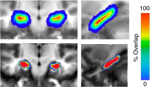
Figure depicts anatomical variability of human hippocampus for 15 normal subjects. in both coronal (left) and sagittal (right) cropped sections. The top row shows the averaging of segmentations of the 15 participants which have been Talairach aligned. The bottom row shows the segmentation agreement after LDDMM alignment. The overlaid colors range from red (all participants agree for that voxel) to blue (one participant labels this voxel in the template as part of the hippocampus).

The bottom row of Fig. 6 (right column) demonstrates the anatomical agreement after LDDMM alignment based on the segmentations. The overlaid color being almost completely red implies that all participants agree on almost all the template voxels after LDDMM alignment. The only disagreement – yellow turning to blue – occur at the boundary of the hippocampus. The results indicate that the high local dimensions of LDDMM provide increased power in terms of accommodating anatomical variation. As illustrated in the functional anatomy section, the accurate registration increases statistical power in fMRI studies.

Time series

The time-series models have been discussed previously for dense imagery for continuous observation (Miller, 2004). Beg has examined the case when given discrete time samples during the atrophy process.

Proposition 2

Given smooth template I_temp=I_t0 denoting the template corresponding to the baseline image, with observations I^(t_k), k=1… N image time-points representing the longitudinal time-sequence, with flow minimizing the variational problem

$${\int }_0^T{\parallel {\mathit{v}}_t\parallel }_V^{2}dt+\gamma \frac{1}{N}\sum _{k=1}^N{\parallel I_{t_0}\left(g_{t_k}^{-1}\right)-I^{\left(t_k\right)}\parallel }^2,$$ (23)

has momentum satisfying

$$M_t=\frac{\gamma }{N}\sum _{k=1}^N{1}_{[0,t_k]}\left(t\right)\mid D{g}_{t,t_k}\mid \left(I_{t_0}\left(g_t^{-1}\right)-I^{\left(t_k\right)}\left(g_{t,t_k}\right)\right)\nabla \left(I_{t_0}\left(g_t^{-1}\right)\right),$$ (24)

with 1_A(t) the indicator function with value 1 if t∈A.

Khan and Beg (2008) have examined the longitudinal growth model in the caudate nucleus of a Huntington's disease patient scanned on five separate occasions over a 71 month period in intervals of 24, 13, 8 and 26 months. Manual segmentations of the left and right caudate nucleus were used, smoothed with a Gaussian convolution filter (mask size: 5×5, σ=1), and discretized the longitudinal time-flow proportional to the actual time-between scans as one time-step per month. Segmentations of the left and right structures are combined into a single image volume (76×80×48) with image time-point rigidly registered to the baseline image. Fig. 7 shows the evolution of the template image along the time-flow and the corresponding input data.

Fig. 7.

Longitudinal growth model results for Huntington's Disease examining the caudate nucleus (Khan and Beg, 2008) where the subject has been scanned five times over the course of six 6 years. The time-flow is discretized to satisfy 20 time-steps per year. Input shapes are shown along with the baseline shape as deformed along the flow, colored with $\mid D{g}_t^{-1}\mid$, with values below 1 indicating localized loss of tissue.

The random orbit model and template estimation

Population study of functional and structural response always involve extrinsic coordinate systems, i.e. atlases or templates. Throughout this section we shall assume the random objects I ∈I are dense scalar images, and we will model them as conditional Gaussian random fields centered around the template. This is a local model in shape space, local to the template. Concurrently work is proceeding on developing these random models for surfaces as well.

The random orbit

The momentum conservation indicates that the momentum M_t=Av_t along the geodesic is conserved (Miller et al., 2006), implying the initial momentum M₀ encodes the geodesic connection. This reduces the problem of studying shapes of a population in a nonlinear diffeomorphic metric space to a problem of studying the initial momenta in a linear space (Vaillant et al., 2004). This momentum parameterization is the basis for our Miller–Trouve–Younes (MTY) random orbit model on shapes which we now describe.

We take as elements anatomical configurations I ∈I, functions indexed over X ⊂R³, I(x), x∈X. We assume the orbit is generated from an exemplar I_temp∈I. The template is unknown and must be estimated. All elements I ∈I are generated by the flow of diffeomorphisms from the template for some g_t, I=g₁ · I_temp.

As illustrated in Fig. 8, our random model has two parts. The first part assumes the anatomies I⁽ⁱ⁾∈I, i=1, 2, …, n, are generated via geodesic flows of the diffeomorphism equation ${\stackrel{.}{g}}_t^{\left(i\right)}={\mathbf{v}}_t^{\left(t\right)}\left(g_t^{\left(i\right)}\right)$, t∈[0, 1] from I_temp, so that the conservation equation holds and the flow satisfies the conservations of momentum. Thus, when ${\mathrm{M}}_0^{\left(i\right)}$, i=1, 2, …, n are considered as hidden variables, our probability law on I⁽ⁱ⁾∈I is induced via the random law on the initial momenta ${\mathrm{M}}_0^{\left(i\right)}$ in a linear space, which are modeled as independent and identically distributed Gaussian random fields (GRF) with zero mean and covariance matrix K/λ. The second part is the observable data I^D(i)∈I, the medical imagery. We assume the I^D(i) are conditional Gaussian random fields with mean fields $I^{\left(i\right)}\circ g_1^{\left(i\right)-1}$ with variance σ². The goal is to estimate the template I_temp and σ² from the set of observables I^D(1), I^D(2), …I^D(n).

Fig. 8.

Random orbit model of dense imagery. The momentum M₀ is modeled as a Gaussian random field, inducing the probability law on images I generated as random deformations of the template. The observed MRI imagery I^D are conditionally Gaussian random fields with mean field g·I_temp.

The EM algorithm for template construction

Study of responses in populations involve atlases or template. For constructing templates from populations of dense imagery, we follow Ma et al. (2008). Given measured anatomical data sets I^D(i), i=1, …, n, with unknown mean field $I^{\left(i\right)}=g_1^{\left(i\right)}\cdot I_{\mathit{temp}}$, our goal is to estimate the unknown template I_temp and σ². To solve for the unknown template, an ancillary initial template, I₀, is introduced so that our template is generated from it via the flow of diffeomorphisms of g_t such that I_temp=g₁ · I₀. Realizations from the random momentum process M₀ are denoted m₀. We use the Bayesian strategy to estimate initial momentum m₀ from the set of observations I^D(i), i=1, …, n by computing the maximum a posteriori (MAP) of f(m₀|I^D(1), I^D(2), … I^D(n). To estimate f(m₀|I^D(1), I^D(2), … I^D(n), we include $m_0^{\left(1\right)},\cdots m_0^{\left(m\right)}$ associated with $g_1^{\left(i\right)}$, i=1,2, …n as hidden variables with K₀ and K the covariances of m₀, $m_0^{\left(i\right)}$, respectively, that are known and correspond to the kernel of Hilbert space of velocity fields. Thus, the log-likelihood of the complete data ($m_0,m_0^{\left(i\right)},I^{D\left(i\right)},i=1,2,\dots ,n$) is written as

$$\begin{array}{cc}\hfill \log & f\left(m_0,{\sigma }^2,m_0^{\left(1\right)},\dots ,m_0^{\left(n\right)},I^{D\left(1\right)},\dots I^{D\left(n\right)}\mid I_0\right)=-\lambda {\langle m_0,{\mathbf{K}}_0^{-1}{m}_0\rangle }_2\hfill \\ \hfill & -\sum _{i=1}^n\left\{{\langle m_0^{\left(i\right)},{\mathbf{K}}^{-1}{m}_0^{\left(i\right)}\rangle }_2+\frac{1}{{\sigma }^2}{\parallel I_0\circ g_1^{-1}\circ g_1^{\left(i\right)-1}-I^{D\left(i\right)}\parallel }^2+n\log {\sigma }^2\right\},\hfill \end{array}$$ (25)

where I₀ is the initial template and I^D(i) is the i-th subject. The paired (g_t, m₀) and ($g_t^{\left(i\right)},m_0^{\left(i\right)}$) satisfy the shooting equation (Miller et al., 2006). σ² estimates the variance of the difference between $g_1^{\left(i\right)}\cdot g_1\cdot I_0$ and I^D(i) among n subjects.

The E-step computes the expectation of the log-likelihood of the complete data given the old template $m_0^{\mathit{old}}$ and variance σ^2old

$$\begin{array}{cc}\hfill Q& \left(m_0,{\sigma }^2\mid m_0^{\mathit{old}},{\sigma }^{2\mathit{old}}\right)=-\lambda {\langle m_0,{\mathbf{K}}_0^{-1}{m}_0\rangle }_2\hfill \\ \hfill & -\sum _{i=1}^n{E}_f\left\{{\langle m_0^{\left(i\right)},{\mathbf{K}}^{-1}{m}_0^{\left(i\right)}\rangle }_2+\frac{1}{{\sigma }^2}{\parallel I_0\circ g_1^{-1}\circ g_1^{\left(i\right)-1}-I^{D\left(i\right)}\parallel }^2+n\log {\sigma }^2\right\},\hfill \end{array}$$ (26)

The M-step generates the new template by maximizing the Q-function with respect to m₀, σ², giving the update equation

$$\begin{array}{cc}\hfill & {(m_0,{\sigma }^2)}^{\mathit{new}}=\arg \underset{m_0,{\sigma }^2}{\min }\lambda {\langle m_0,{\mathbf{K}}_0^{-1}{m}_0\rangle }_2\hfill \\ \hfill & +\sum _{i=1}^n{E}_f\left\{\frac{1}{{\sigma }^2}{\parallel I_0\circ g_1^{-1}\circ g_1^{\left(i\right)-1}-I^{D\left(i\right)}\parallel }^2\right\}+n\log {\sigma }^2,\hfill \end{array}$$

and with $E_f\left\{{\langle m_0^{\left(i\right)},K^{-1}{m}_0^{\left(i\right)}\rangle }_2\right\}$ a constant this yields

$${\sigma }^{2\mathit{new}}=\frac{1}{n}\sum _{i=1}^n{\parallel I_0\circ g_1^{-1\mathit{old}}\circ g_1^{\left(i\right)-1}-I^{D\left(i\right)}\parallel }^2,$$ (27)

$$m_0^{\mathit{new}}=\arg \underset{m_0}{\min }\lambda {\langle m_0,{\mathbf{K}}_0^{-1}{m}_0\rangle }_2+\frac{1}{{\sigma }^{2\mathit{new}}}{\parallel ({\stackrel{‒}{I}}_0-I_0\circ g_1^{-1})\sqrt{\alpha }\parallel }^2,$$ (28)

$$\text{where}{\stackrel{‒}{I}}_0=\frac{\sum _{i=1}^n{I}^{D\left(i\right)}\circ g_1^{\left(i\right)}\mid d{g}_1^{\left(i\right)}\mid }{\sum _{i=1}^n\mid d{g}_1^{\left(i\right)}\mid }\text{and}\alpha =\sum _{i=1}^n\mid d{g}_1^{\left(i\right)}\mid .$$

Shown in Fig. 9 are the results of generating a template of multiple subcortical structures including the hippocampus and basal ganglia. Depicted next to each set of structures are the metric distances from the initial template to the final resulting template.

Fig. 9.

Panels show template of multiple structures including hippocampus and basal ganglia (pallidus, caudate, putamen) along with metric distances between the initial template and targets in the population as well as the EM algorithm generated template and the shapes in the population.

Shown in Figs. 10 are the heart templates generated from the initial templates. Depicted on the metric distances between the template and each element of the population are shown with the second number the converged metric distance.

Fig. 10.

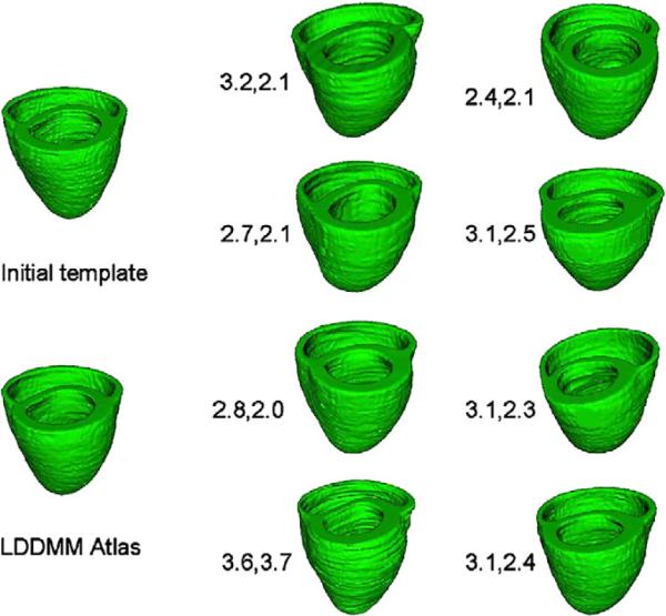
Panels shows heart population and heart template along with metric distances between the initial template and the resulting template.

Transferring functional and physiological variables via group action

In CFA, the study of functional signals in common anatomical coordinates is defined by the way the functional signals are carried by the bijective transformation between coordinate systems g:X↔X^atlas. We denote all the signals, scalars, vectors, tensors as F∈F indexed over the anatomical manifolds X⊂R³, with F(x),x∈X. The principal challenge is the fact that the structures of anatomy are curvilinear, and anatomical structures from one subject to another are not the same shape.

This approach understands the functional statistics of populations in the coordinate of the atlas X^atlas by applying dense diffeomorphisms carrying the physiological signals g:F↦g·F.

Group actions for transferring scalar information

Our group has used group actions for transferring scalar and vector valued information. When the functional information is dense imagery, then the group action used is the right action by the inverse.

Proposition 3

Let F be dense scalar imagery, then

$$g\cdot \mathbf{F}\doteq \mathbf{F}\circ g^{-1};$$ (29)

this is a group action.

Transfer of fMRI bold response into atlas coordinates

Such group actions may be used for transferring fMRI responses into common coordinates. Fig. 11 depicts such an example in the medial temporal lobe depicting the high resolution structural coordinates associated with the MRI coupled to the within subject functional MRI (fMRI) response. The overall approach carries the fMRI response from the population into the atlas or template coordinates.

Fig. 11.

Figure depicts the procedure for transferring or transporting via the diffeomorphisms the within subject fMRI functional responses back to the template coordinates M^atlas via the dense correspondence diffeomorphisms g. The structures shown here are from the medial temporal lobe (Ceritoglu, 2008).

To demonstrate the use of LDDMM mapping for transferring the functional information, shown in Fig. 12 are the basal ganglia structures being studied in an fMRI study. The left column shows the structures for one of the subjects; the middle column show the template structural coordinates.

Fig. 12.

Columns 1 and 2 show structural representations in the target and template, respectively, for the basal ganglia structures. Column 3, top panel shows the functional map after transfer via the bijection into the template coordinates g·fMRI; bottom panel shows a section through the bijection on the coordinate system.

Shown in the right column of Fig. 12 are the associated fMRI signal transferred via the bijection into atlas coordinates (top row) along with the change in coordinate system (bottom row).

Transferring bold response in populations of functional memory task in the medial temporal lobe

We now examine population averaging of the functional MRI responses in template or atlas coordinates associated with memory tasks in the medium temporal lobe (MTL). The major difficulty for fMRI study in subregions of the brain is that structures demonstrate significant variability across individuals. Stark et al. (2004), Miller et al. (2005), and Kirwan et al. (2007) have been examining the MTL in responses to memory tasks in the medial temporal lobe (MTL) in populations of normals.

Shown in Fig. 13 are results of LDDMM-image mapping of the MTL structures. The left panel shows the MTL structures which were registered with the functional response transferred via the group action of the bijection to template coordinates. The right panel shows the hemodynamic response from a 39-voxel (609 mm³) cluster within the right perirhinal cortex (voxel-wise p<0.02) following Talairach and LDDMM transformations. The beta coefficient (magnitude of response) is plotted representing the general linear model's estimate of the fMRI activity as a function of time associated with incidental encoding of stimuli during the memory retrieval task. This result demonstrates the enhancement of the activity within the region itself using LDDMM alignment versus Talairach. A similar fMRI study in the auditory cortex has been done by other researchers and shown good separation of functional activities using LDDMM-landmark mapping when comparing with spherical registration (Desai et al., 2005).

Fig. 13.

Left panel shows the MTL structures studied including the hippocampus (red), temporopolar cortex (green), perirhinal cortex (yellow), entorhinal cortex (blue), and parahippocampal cortex (cyan). Right panel plots the hemodynamic responses as represented by the beta coefficient of response from a 39-voxel (609 mm³) cluster within the right perirhinal cortex following Talairach (left) and LDDMM (right) (Stark et al., 2004; Miller et al., 2005; Kirwan et al., 2007).

Transferring vectors and DTI matrices via group action in the heart and brain

Often times the functional information is either vector or matrix information. Now examine vector and tensor information from diffusion tensor imaging applications.

When the functional information are tensor matrices, then we use the action of Alexander and Gee (2000) preserving the determinant using the Gram–Schmidt orthogonalization.

Proposition 4

1. Let F be a 3×3 tensor matrix, then with F having eigenelements λ_i, e_i, i=1,2,3, the action is defined by $g\cdot \mathbf{F}\doteq ({\lambda }_1{\widehat{e}}_1{\widehat{e}}_1^t+{\lambda }_2{\widehat{e}}_2{\widehat{e}}_2^t+{\lambda }_3{\widehat{e}}_3{\widehat{e}}_3^t)\circ g^{-1}$ where

$${\widehat{e}}_1=\frac{Dg{e}_1}{\parallel Dg{e}_1\parallel },{\widehat{e}}_2=\frac{Dg{e}_2-\langle {\widehat{e}}_1,Dg{e}_2\rangle {\widehat{e}}_1}{\sqrt{{\parallel Dg{e}_2\parallel }^2-{\langle {\widehat{e}}_1,Dg{e}_2\rangle }^2}},{\widehat{e}}_3={\widehat{e}}_1\times {\widehat{e}}_2.$$ (30)

Let F be the 3×1 first eigenelement vector λ₁e₁ of the diffusion tensor matrix, the action is defined by $g\cdot \mathbf{F}\doteq \left({\lambda }_1{\widehat{e}}_1{\widehat{e}}_1^t\right)\circ g^{-1}$ where

$${\widehat{e}}_1=\frac{Dg{e}_1}{\parallel Dg{e}_1\parallel }.$$ (31)

These are group actions.

DTI vector information in brain development

Lee and Mori (2008) have been studying growth, examining the contrast changes in the imagery independent from the geometric changes. To study changes during growth the eccentricity of the principal eigenvectors are reconstructed in the template coordinates. The diffeomorphisms are used to transfer the DTI vector images according to the group actions of Eqs. ((30)–(31)). To accomplish this 237 fiducial points were defined in each of a time sequence of brains along with the corresponding 18 year old template. The LDDMM landmark procedure was carried out for each brain. The diffeomorphism was used to carry the DTI imagery into the template coordinates using the vector group action from which registered imagery was generated for comparing the DTI contrasts independent of the geometric changes of the tissue.

Fig. 14 depicts the transport of DTI myelination response variables as encoded via the eccentricity of the eigenvectors of the DTI tensor. Shown are time samples 0, 7, 24, 36, and 60 months of original section (top row) then carried via bijection into template coordinatese (bottom row). Here the bijective correspondence is transporting the DTI eccentricity measure to the template coordinates for statistical examination.

Fig. 14.

Transfer of DTI myelination response variables as encoded via the eccentricity of the eigenvectors of the DTI tensor. Top row shows are 0, 7, 24, 36, and 60 month time samples via color coding of the principal eigenvector. The bottom row shows the color coding of the principal eigenvector in the DTI. Here the bijective correspondence is transforming the principal axis via group action on the vector carried into the template coordinates. Data taken from the laboratory of Dr. Susumu Mori of Johns Hopkins University.

DTI matrix information in the heart

Many groups have been examining the structure and function of the heart at multiple scales. Fig. 15 shows results from recent efforts of Beg et al. (2004), Helm et al. (2006) and Helm et al. (2005) from exvivo dog hearts upon which high resolution structural MRI and DTI was performed. In the top row, panels 1 and 2 show normal hearts, and panel 3 shows a failing heart. Notice the variability of global size as well as local structural shape. Each of the normal and abnormal hearts were mapped to a common extrinsic atlas using LDDMM-image mapping, from which principal components were calculated on the initial momentum Av₀.

Fig. 15.

Top row shows sections through the 3D hearts depicting heart variability in the anatomical sections. The bottom left panel shows the method for calculating the relative wall thickness RWT=h/r parameters. Rightmost block of panels depicts the RWT superimposed in atlas coordinates of the normal population (top row) and the abnormal population (bottom row) (Beg et al., 2004; Helm et al., 2006; Helm et al., 2005).

The bottom left panel shows the method for calculating the relative wall thickness RWT = h/r parameters. Rightmost block of panels depicts the RWT superimposed in atlas coordinates of the normal population (top row) and the abnormal population (bottom row).

Parallel transport of metric information between multiple templates

The basic questions we examine in this section is how to transport information between multiple local representations in shape space, i.e. between templates that each represent subpopulations. We have already seen that transporting information via bijections is nuanced, we might even say tricky. For points it is left action similar to matrices acting on vectors g:x ↦ g(x), for dense imagery viewed as functions it acts on the right via the inverse g:I ↦ I ° g⁻¹, and for DTI matrices it is defined to preserve the determinant and to rotate the eigenfunctions based on the orthogonalization procedure.

We now examine the cases for transferring vector fields in the tangent space associated with the template, along with their associated inner product, for example when we have multiple templates with their eigenfunction representations.

We have studied at least two cases involving transfer of metric information between template representations of populations. The first one arises when studying different cohorts of groups and or illnesses where there are multiple templates with different eigenfunctions. The question becomes how do we share that information from one template to another. Fig. 16 depicts the multiple template case for different population cohorts and illnesses. Panel 1 shows the EM algorithm generated hippocampus template generated in the BIRN study (Miller et al., 2008) from a population of 101 hippocampi which were segmented using FreeSurfer. The vector fields and principal components were determined for studying morphometric change of the Alzheimer's population. Superimposed are the metric distances between template and population. Panel 2 shows the Csernansky template used in hippocampus studies for schizophrenia. The natural question is how do we share template centered information.

Fig. 16.

Shown in panel 1 is a sample population of hippocampi from the BIRN study (Miller et al.2008) of an Alzheimer's population with generated template and metric distances between the subpopulation of shapes and the template. Shown in panel 2 is the Csernansky template used for studying the schizophrenia population along with a depiction of the vector information determining the effect size for separating the two populations.

The second scenario occurs for growth and or atrophy in which each time series naturally carries its own template which optimally represents the within subject sequence variation; we call this the subject's anatomical coordinate system. In the obvious sense, you are your own best template. The question becomes then how do we perform population averages across sequences when there are multiple subject anatomical coordinate systems. Depicted in Fig. 17 are a sequence of hippocampi observed over time (Qiu et al., in press). The first element in each sequence is used as the subject's anatomical coordinate system (template).

Fig. 17.

Framework for handling growth and atrophy with multiples subjects each corresponding to a different sequence. The first element in each time series is taken as the template for its sequence. LDDMM geodesic connection is calculated between each element in the sequence with its own template (Qiu et al., in press). Parallel transport is used to transform all of the geometric information encoded in each subject's sequence template to the common hypertemplate which collects all of the results (Qiu et al., in press) in the population.

In Euclidean space, the operation of transferring vector fields is the standard translation of vectors. In curved spaces such as shape space, we use parallel transport following the original developments of Younes based on Jacobi fields (Younes, 2007) (see Younes et al., 2008; Qiu et al., in press) for derivations of algorithms for computing parallel transport for point-sets). The coordinate system which collects the information we call the hypertemplate. Parallel transport is used since it has the advantage that the vector information (such as the momentum) encoding each of the sequences is transferred to the common hypertemplate coordinate system so that the metric (inner products on the vector information being transferred) is maintained. Therefore inner products associated with principal components and random fields representations will be preserved when transferred to the hypertemplate. We shall focus solely on point-set transfer of the metric information here; for transferring the dense imagery this is described in Younes et al. (2008).

Parallel transport of point sets

The goal is to calculate F_t,t∈[0, 1], F₀ = F, which transports the metric vector field information F along the geodesic flows h_t,t∈[0, 1] connecting the within subject sequences to the hypertemplates. Throughout assume the kernel is diagonal K(x,y)=k(x,y)id, id a 3×3 identity matrix, and we use the shorthand notation h_it=h_t(x_i) to denote the location of a particle in the point-set x_i at time t. The geodesic connection to the hypertemplate, h_t and the ODE Eq. (11) simplifies to

$$\frac{\mathrm{d}}{\mathrm{d}t}{h}_{it}={\mathit{v}}_t\left(h_{it}\right)=\sum _{j}k(h_{jt},h_{it}){\alpha }_{jt},$$ (32)

$$\frac{\mathrm{d}{\alpha }_{it}}{\mathrm{d}t}=-\sum _j{\nabla }_{1}k(h_{it},h_{jt}){\alpha }_{jt}^{\ast }{\alpha }_{it}.$$ (33)

In curved spaces such as described by the geodesics in shape space, the principal tool Younes introduced for parallel transport of the vector fields along the geodesics so as to preserve the inner products are perturbation of the exponential maps by the vector fields being transported given by the Jacobi field (Younes, 2007; Younes et al., 2008).

Younes's idea for generating the transport is given F_t the transport of F to time t, then for small s, ${\mathbf{F}}_{t+s}~\frac{J_{t+s}}{S}$ with J the Jacobi field to perturbation direction F_t. The Jacobi field is the directional derivative of the geodesic; perturbing v_t→v_t+εδv_t gives the perturbation of the geodesic flow h_t→h_t+εδh_t. The Jacobi field is the ε limit and therefore a tangent vector to the curve.

Since we are in the point setting, the vector fields are parameterized in their local coordinate representation involving the particle paths with the perturbations in terms of the perturbation of the particle momenta. The Jacobi field is calculated via the perturbation α→α+εδα of the flow Eq. (32) giving

$$\begin{array}{cc}\hfill \frac{\mathrm{d}}{\mathrm{d}s}{J}_{it+s}& (\alpha ,\mathbf{F}){{\mid }_t={\mathbf{F}}_t\frac{\mathrm{d}}{\mathrm{d}s}\delta h_{it+s}(\alpha ,\mathbf{F})=\frac{\mathrm{d}}{\mathrm{d}\epsilon }\mid }_{\epsilon =0}\sum _{j}k\left(h_{jt+s}^{{\alpha }_t+\epsilon \delta {\alpha }_t},h_{it+s}^{{\alpha }_t+\epsilon \delta {\alpha }_t}\right)\hfill \\ \hfill & \times ({\alpha }_{jt+s}+\epsilon \delta {\alpha }_{jt+s})=\sum _j({\nabla }_1^{\ast }k(h_{jt+s},h_{it+s})\delta h_{jt+s}\hfill \\ \hfill & +{\nabla }_2^{\ast }k(h_{jt+s},h_{it+s})\delta h_{it+s}){\alpha }_{jt+s}+\sum _{j}k(h_{jt+s},h_{it+s})\delta {\alpha }_{jt+s},\hfill \end{array}$$ (34)

with $\frac{\mathrm{d}}{d_s}{J}_{\mathit{it}+s}(\alpha ,\mathbf{F})\mid t={\mathbf{F}}_t$. The ODE on the local coordinate evolution δα_js+s is computed according to the perturbation of Eq. (33) given by

$$\begin{array}{cc}\hfill \frac{\mathrm{d}}{\mathrm{d}s}\delta {\alpha }_{it+s}& =-\frac{d}{d\epsilon }{\mid }_{\epsilon =0}\sum _j{\nabla }_{1}k\hfill \\ \hfill & \times \left(h_{it+s}^{{\alpha }_t+\epsilon \delta {\alpha }_t},h_{jt+s}^{{\alpha }_t+\epsilon \delta {\alpha }_t}\right)({\alpha }_{jt+s}+\epsilon \delta {\alpha }_{jt+s})\ast ({\alpha }_{it+s}+\epsilon \delta {\alpha }_{it+s})\hfill \\ \hfill & =-\sum _j({\nabla }_1^{\ast }{\nabla }_{1}k(h_{it+s},h_{jt+s})\delta h_{it+s}+{\nabla }_2^{\ast }{\nabla }_{1}k(h_{it+s},h_{jt+s})\delta h_{jt+s})\hfill \\ \hfill & \times {\alpha }_{jt+s}^{\ast }{\alpha }_{it+s}-\sum _j{\nabla }_{1}k(h_{it+s},h_{jt+s})\left(\delta {\alpha }_{jt+s}^{\ast }{\alpha }_{it+s}+{\alpha }_{jt+s}^{\ast }\delta {\alpha }_{it+s}\right).\hfill \end{array}$$ (35)

The algorithm becomes, given F_t the transported vector F to time t, then F_{t + s} for small s is computed from the Jacobi field with the algorithm cycling to the next small increment.

Hippocampal atrophy at two time points

We present a longitudinal study on hippocampal shape in aging and AD to demonstrate the use of parallel transport in time-dependent anatomical characterization for assessing disease stages (Qiu et al., 2008). Hippocampal surface structure was assessed twice two years apart in 26 nondemented subjects (CDR 0), in 18 subjects with early AD (CDR 0.5), and in 9 subjects who converted from the nondemented (CDR 0) to the demented (CDR 0.5) state. The objective was to distinguish converters from healthy subjects and subjects with AD using the pattern of hippocampal shape changes during the two-year time interval.

All hippocampi were delineated. We assessed within-subject hippocampal shapes at the two time points using LDDMM-surface mapping. We translated the within-subject hippocampal shape variation from the subject's anatomical coordinate system to the hypertemplate coordinate system using parallel transport for statistical testing. Our results from random field analysis revealed that inward surface deformation across time occurred in a non-uniform manner across the hippocampal surface in subjects with early AD relative to the healthy controls. As illustrated in Fig. 18, the lateral aspect of the left hippocampal tail showed inward surface deformation in the converters and whole hippocampal body showed inward surface deformation in the early AD when compared with the healthy controls. Using surface deformation patterns as features in a classification analysis, we were able to respectively distinguish converters and patients with early AD from healthy controls at classification rates of 0.77 and 0.87.

Fig. 18.

Statistically significant shape difference between diagnostic groups. The warm color denotes that the outward surface deformation in the former group relative to the latter group, while the cool color corresponds to inward surface deformation. The color bar indicates the strength of the surface deformation in terms of the local rate of volume loss during the two year period.

Signal processing and statistical inference in anatomical coordinates

Performing classical signal filtering, smoothing and statistical inference on the physiological signals F∈F on curved manifolds X is challenging. We unify these issues by essentially constructing the Hilbert space, H(X), in the anatomical coordinate X with the physiological signals elements F∈H(X). The construction of H(X) requires the generation of a complete orthonormal (CON) base {ϕ(·)} indexed over X. Given such a base then least-square smoothing and splines on X all become available. In the statistical testing, our observations include both anatomical manifold X and physiological signal F defined on X, (F, X). The analysis for understanding the functional and structural pair (F, X) is to place them in atlas coordinates X^atlas via the dense diffeomorphism g:X→X^atlas, the mapping of tha anatomical manifold X to the atlas X^atlas. For each pair (F, X), g is applied according to g:(F,X)→(F^atlas, X^atlas). Thus, given a basis ϕ(x), x∈X^atlas and diffeomorphism g, statistical inference via random fields built on the atlas coordinates becomes convenient.

We model the physiological and structural signals F(x), x∈X⊂R^d indexed over the manifolds as arising from a Hilbert space, F, with inner product and a complete set of orthonormal bases ϕ. For all F∈F, we have

$$\mathbf{F}\left(x\right)=\sum _i{\mathbf{F}}_i{\varphi }_i\left(x\right),x\in X,\sum _i{\parallel {\mathbf{F}}_i\parallel }^2<\infty .$$ (36)

Constructing the Hilbert space F in local anatomical coordinates

We have two ways of generating complete orthonormal (CON) bases in submanifolds. The first which we shall describe and have used extensively for surfaces is based on the eigenfunctions of the Laplace–Beltrami operator. The second approach is to directly perform principal component analysis (PCA) thereby generating the “principal components” which describe anatomical variation with respect to a privileged CON base.

First examine CON bases generated with self-adjoint differential operators. Since many of the manifolds of CFA are volumes and surfaces the differential operator used for inducing the orthonormal basis is the generalization to the Laplace–Beltrami operator (Qiu et al., 2006). In cubic volumes and on the sphere it is complex exponentials and spherical harmonics.

Proposition 5

Given smooth manifold X⊂R^d, then eigenfunctions of the Laplace–Beltrami (LB) operator solving the spectral problem below generate a complete set of orthonormal bases in the Hilbert space F on X⊂R^d.

The LB spectral problem with Neumann boundary conditions for X is posed as

$$\begin{array}{cc}\hfill \Delta \varphi +\lambda \varphi & =0,\text{on}X,\hfill \\ \hfill {\int }_X{\mid \varphi \left(x\right)\mid }^2\mathrm{d}x& =1,\hfill \\ \hfill \langle \nabla \varphi (\cdot ),\overrightarrow{n}\rangle {\mid }_{\partial X}& =0,\hfill \end{array}$$ (37)

where Δ is the LB operator, with $\overrightarrow{n}$ the normal vector on the boundary of X. Such bases ϕ are only dependent on the geometry of X.

Fig. 19 shows examples of the first several eigenfunctions of open surfaces the occipital (top row) and central sulcus (bottom row)

Fig. 19.

Top rows shows eigenfunctions of the Laplace–Beltrami operator generated from the open surfaces the occipital cortex; bottom row shows the central sulcus. The central sulcus is shown in planar coordinates because it is highly curved. The regions change in sign from red to blue.

Shown in Fig. 20 are eigenfunctions from closed surfaces including the hippocampus, putamen amygdala and globus pallidus.

Fig. 20.

Rows show eigenfunctions of the Laplace–Beltrami operator generated from closed surfaces including the hippocampus, putamen, amygdala and globus pallidus.

Principal components in anatomical coordinates

Now examine the second method for generating complete orthonormal (CON) bases in submanifolds based on PCA. Fig. 21 shows the first eigenfunction on the hippocampus reconstructed from PCA on vector fields mapping normal elderly subjects to candidates with Alzheimer's disease (Wang et al., 2003). Panel 2 of top row shows the reconstruction in the 1st, 2nd, and 5th eigenfunctions of the differences between the two populations. The second row of Fig. 21 shows the 1st eigenfunction on the thalamus generated from PCA on vector fields mapping controls to schizophrenics (Csernansky et al., 2004). The bottom row shows the reconstructions of the difference between the two population in the 1,8, and 10th eigenfunctions.

Fig. 21.

Top row shows the 1st eigenfunctions of the hippocampus (Wang et al.2003) (panel 1) and difference between normal and Schizophrenics expanded in the 1st, 2nd, and 5th eigenfunctions generated via PCA. The second row shows the first eigenfunction of the thalamus (Csernansky et al.2004) reconstructed from PCA on vector fields mapping normals to Alzheimer's. Row 3 shows the reconstructions in the thalamus in 1st, 8th, and 10th eigenfunctions of the differences between the normals and Alzheimer's (Csernansky et al.2004).

Fig. 22 shows PCA results from the MRI and DTI heart data from Fig. 15 (Beg et al., 2004; Helm et al., 2006; Helm et al., 2005). Each of the normal and abnormal hearts were mapped to a common atlas using LDDMM-image mapping, from which principal components were calculated on the initial momentum M₀ = Av₀. The two rows show geodesic shooting of the momentum according to Eq. (21) using only the first principal component Av₀=αϕ for the normal (top row) and failing populations (bottom row), with α varied from positive to negative one and running the conservation equation for one time unit. These vectors point in the directions of the highest geometric variability. Notice for the normal the variation of the right ventricle insertion point and the change in left ventricular shape. The failing population shows its principal change as ventricular dilation and wall thinning. The bottom two rows of Fig. 22 show evolution of normal template mouse heart within 2 standard deviations (SD) along the direction of highest geometric variance estimated for normal (row 3) and failing mice hearts (row 4) at end systole. The middle column in each row represents the normal template. The far left and right columns in each row represents images synthesized at −2 and +2 SD, respectively. In comparison to the normal population, there are more prominent changes in chamber diameter, wall thickness, and right ventricle insertion point. (The colors were added to enhance structural details and do not represent any quantitative measures.)

Fig. 22.

Top two rows show geodesic shooting of the momentum using only the principal component M₀=Av₀=αϕ for the normal (row 1) and failing ex-vivo populations (row 2), with α varied from positive to negative one and running the conservation equation for one time unit (Helm et al., 2006; 2005). Bottom two rows show evolution of normal template mouse heart within 2 standard deviations (SD) along the direction of highest geometric variance estimated for normal (row 3) and failing mice hearts (row 4) at end systole. The middle column in each represents the normal template. The far left and right columns in each row represents images synthesized at −2 and +2 SD, respectively.

Spline interpolation in anatomical coordinates

Processing the signals directly in the local coordinates is powerful because it represents the local geometry. For smoothing and filtering, distances within the anatomical structure are preserved and respected. In the case of the brain, signals far away in gyral or sulcal length should not be averaged, or only averaged weakly. The classical spline model takes the following form on F.

Proposition 6

Spline Interpolation Problem Let Y(x), x∈X be the observation of F(x), x∈X with mean field μ_F and covariance $\mathbf{K}={\Sigma }_i\frac{1}{{\lambda }_i}{\varphi }_i{\varphi }_i^{\ast }$, where ϕ is the orthonormal basis of the Hilbert space H(X^atlas). Then the “smoothed spline representation” of F given by

$$\widehat{\mathbf{F}}=\arg \underset{{\mathbf{F}}_i:\mathbf{F}=\sum _i{\mathbf{F}}_i{\varphi }_i}{\min }{\parallel Y(\cdot )-\sum _i{\mathbf{F}}_i{\varphi }_i(\cdot )\parallel }^2+\langle \sum _i{\mathbf{F}}_i{\varphi }_i,{\mathbf{K}}^{-1}\sum _i{\mathbf{F}}_i{\varphi }_i\rangle ,$$ (38)

satisfies

$$\widehat{\mathbf{F}}(\cdot )={\mathbf{F}}_0(\cdot )+\sum _{k=1}^n{\beta }_k\mathbf{K}(x_k,\cdot ).$$ (39)

Given X as a 2-dimensional manifold embedded in R³ (e.g., surface), we choose (λ_i, ϕ_i) as the eigenelements of the Laplace–Beltrami operator. The solution to F₀ and β_k is obtained by minimizing

$$\widehat{\mathbf{F}}\left(u\right)=\underset{\mathbf{F}={\mathbf{F}}_0(\cdot )+\sum _{k=1}^n{\beta }_k\mathbf{K}(x_k,\cdot )}{\arg \min }\gamma {\int }_X{\parallel \nabla \mathbf{F}\parallel }^2\mathrm{d}x+\sum _{k=1}^n{(Y_k-\mathbf{F}\left(x_k\right))}^2,$$ (40)

for fixed γ>0.

Fig. 23 depicts the local spline representation of functional responses to ring stimuli in the visual cortex (Qiu et al., 2006). Column 1 shows the occipital cortical reconstruction. Column 2 shows the two ring stimuli used for obtaining the functional maps with a fixation disk at rings' centers. The red circles mark the centers of the rings. Column 3 shows the smoothed functional statistical maps (t-value) for the two different stimuli generated via the spline model on the cortical manifold X using the spline interpolation. Bright color represents the high t-value region, while dark color denotes the low t-value region. The right column show the functional response with the ridge corresponding to the center of the ring tracked using dynamic programming on the planar view (Qiu et al., 2006).

Fig. 23.

Column 1 illustrates the location of the occipital lobe in the brain. Column 2 shows the ring stimulus with fixation disks and center marked by red circles. Columns 3 and 4 show the functional responses on the surface of the visual cortex generated via the spline interpolation solution and in the planar coordinates respectively, with ridges corresponding to the centers of the rings (Qiu et al.2006). Bright color represents the high t-value region, while dark color denotes the low t-value region.

Random field models for statistical analysis

To accommodate a statistical analysis, the most general approach is to consider that observations arise from an infinite dimensional random process (X, F) that includes the manifold X and the physiological signal F that is carried by X. In the extrinsic atlas analysis, (X, F) are studied in a common atlas coordinate system X^atlas via diffeomorphic correspondences g:X→X^atlas. The random field modeling performs hypothesis testing in the coordinates of the atlas.

Proposition 7

Given atlas X, and associated orthonormal bases ϕ(x), x∈X^atlas, let F transformed by g to X^atlas be modeled as

$$\mathbf{F}\circ g=\sum _i{\mathbf{F}}_i{\varphi }_i,$$ (41)

then in extrinsic analysis with F₁, F₂,… Gaussian variables, F on X^atlas is a Gaussian random field with mean and covariance induced according to

$${\mu }_{\mathbf{F}}=\sum _{i}E\left({\mathbf{F}}_i\right){\varphi }_i,{\mathbf{K}}_{\mathbf{F}}=\sum _{ij}E\left({\mathbf{F}}_i{\mathbf{F}}_j\right){\varphi }_i{\varphi }_j^{\ast }.$$ (42)

This is a powerful methodology for analyzing brain function since the choice of the basis ϕ is done once for the atlas, and then transported to the observed manifolds. In this approach of course the inference depends on the implemented registration algorithm. In Qiu's thesis work (Qiu, 2006) intrinsic methods were studied which are independent of the diffeomorphic mapping.

Alzheimer's shape change via momentum mapping in atlas coordinates

The geodesics determining the metric in the LDDMM connection of one shape to another is encoded via the initial momentum denoted M₀ (Miller et al., 2006). It is natural to compute the statistically significant locations of the shape change between the populations as characterized by these initial vector fields. The Av₀ completely determines the LDDMM maps from the atlas onto the target shapes. The initial momentum has the added attractive property that it is normal to the level lines of the atlas (Miller et al., 2006). For surface mapping it is normal to the atlas surface and specified by a scalar field indexed over it according to

$$M_0\left(x\right)=\mu \left(x\right)N\left(x\right),x\in X^{\mathit{atlas}},$$ (43)

with N(·) is the normal field to the surface. Population shape variation is represented by the length of the scalar fields μ(x),x∈X^atlas with positive sign pointing outward motion and negative pointing inward motion relative to the atlas coordinates. For statistics we model μ(x), as a Gaussian field in the form of

$$\mu \left(x\right)=\sum _k{U}_k{\varphi }_k\left(x\right),x\in X^{\mathit{atlas}},$$ (44)

where the U_k are Gaussian random variables and ϕ_k(x) are chosen as the k-th eigenfunction of a complete orthonormal base generated from the Laplace–Beltrami operator on X^atlas (Qiu et al., 2006). The eigenfunctions for the hippocampus are exemplified by those depicted in the top row of Fig. 20.

Using the scalar of the initial momentum and Gaussian random field model, we studied hippocampus shape change in Alzheimer's disease in population of 57 healthy elder controls (age: 75.5±7.72, 31 males and 26 females) and 38 patients with very mild Alzheimer's patients (age: 73.6±5.98, 23 males and 15 females). We estimated an atlas from the population (Ma et al., 2008) and deformed it to all hippocampi in the study using LDDMM-surface mapping to obtain initial momenta. Then the initial momentum from each hippocampus was modeled as Gaussian field on the atlas in Eq. (44). To compare the shape difference between the two populations, two-sample student t-test was performed on each of the first twenty expansion coefficients U_k. The statistically significant group difference occurs in the 1st, 5th, 20th components at a significance level of 0.05. Fig. 24 shows the statistically significant shape differences between the normal and Alzheimer's disease populations constructed in the basis representation indexed over the template coordinate X^atlas. The warm and cool colors respectively denote regions where the hippocampus has compressed or expanded in the Alzheimer's population. The statistical results suggest that the subiculum of the hippocampus is most affected by the disease.

Fig. 24.

Panel (a) shows statistically significant shape difference expanded in the three statistically significant coefficients Σ_k∈{1,5,20}U_kϕ_k between 38 patients with Alzheimer's disease and 57 comparison controls. Panels (b,c) show statistically significant shape differences using subsets of sample subjects. Red color denotes the region where the hippocampus is compressed; blue is the region where the hippocampus is expanded in the group of patients with Alzheimer's disease.

To quantify the reliability of the method, we split subjects into two subsets. The first subset had 45 subjects including 27 healthy comparison controls and 18 very mild AD patient. The second subset had 50 subjects including 30 healthy comparison controls and 20 very mild AD subjects. Gender and age are matched in the two subsets. We applied the same statistical analysis procedure as described above. Fig. 24 shows results from the two subsets that are in close agreement with the one used from the entire population.

Statistical inference via cortical thickness in planum temporale atlas coordinates for schizophrenia

Cortical thickness F(·)=thickness is a scalar field indexed over the cortical submanifold X⊂R³ which is transferred via to the template. We have been studying cortical thickness variation of the left planum temporale (PT) between 20 healthy comparison subjects and 20 schizophrenia patients (Qiu et al., 2008). The left PT was selected since it is the auditory association cortex responsible for language and speech processing function and has received great attention in schizophrenia research. To investigate the group difference in thickness, we first selected a template from the healthy control group and then applied the LDDMM-surface mapping to deforming the template to all other left PT surfaces. The thickness maps F_thick of each subject were transformed to the template based on the closest vertices on the template to vertices on other surfaces. The average thickness maps within each group are illustrated in columns 1 and 2 of the first row in Fig. 25. Cortical thickness maps indicate that thickness varies across the PT from 1.5 mm to 4 mm. The PT is thin at the bottom of Heschl's sulcus (HS), then progressively thicker away from HS, and finally thinner towards the posterior ramus. The variation in cortical thickness may be related to the geometry of the PT cortical surface in the sense that regions with high curvature (perhaps gyral regions) have larger thickness value while regions with low curvature (sulcal regions) have smaller thickness value. The bottom row of Fig. 25 (c) shows the difference in the average thickness maps between the control and schizophrenia groups.

Fig. 25.

Panels 1 and 2 show the mean cortical thickness maps in the control and schizophrenic groups on the planum temporale. Panel 3 shows the cortical difference between the control and schizophrenic groups. Panel 4 shows the statistically significant group difference (Qiu et al.2008) reconstructed from the basis functions of the Laplace–Beltrami like those shown in Fig. 19.

To investigate the non-uniform changes, we constructed the Gaussian random field (GRF) model on the template as in Eq. (41). The rightmost column shows the second and third basis generated in the template coordinates. Then, the Hotelling's T² test was performed on coefficient vectors under the null hypothesis that the coefficient vectors are equal in both control and schizophrenic groups. Table 1 lists T² statistics and the corresponding p-values shown as a function of the progressive increase in the number of coefficients each time. These p-values determined from F-distribution suggest that the pattern of significant difference in the thickness map between the control and schizophrenic groups is caused by the second basis. Such a pattern can be reconstructed by subtracting the mean coefficient in the schizophrenic group from one in the control group, and then multiplying this basis (see Fig. 25(d)).

Table 1.

The Hotelling's T² statistics and their corresponding p-values for the tests involving the first N coefficients

N	CON vs. SCZ
	$T_N^2$	p-value
1	5.4072	0.0255
2	5.4083	0.0853
3	5.4366	0.1809
4	6.1440	0.2494
5	6.1677	0.3766

Control and schizophrenia are respectively abbreviated as CON and SCZ.

Comparison of random field models and point-wise based testing

Point-wise hypothesis testing has been widely used in neuroimaging studies, including volume-based and surface-based fMRI, cortical thickness and gray matter density (Chung et al., 2005; Genovese et al., 2002) False discovery rate (FDR) (Genovese et al., 2002) and random field theory (RFT) (Chung et al., 2005; Worsley et al., 2004, 1996) approaches are applied to seeking objective and effective threshold for point-wise statistics derived from neuroimaging data. However, the threshold determined by both approaches is dependent on the smoothness of data. In the following, we first explore thickness difference between the healthy comparison control and schizophrenia groups from the point-wise hypothesis testing approach thresholded using FDR or RFT at two different smooth scales. Then, we compare the findings with those using the random field model. The same dataset as one in the previous section was examined. In the point-wise hypothesis testing, we first applied the heat kernel smoothing procedure (Chung et al., 2005) to our thickness data on the left PT template surfaces using smoothing kernel of full width half maximum (FWHM) at levels of 20 mm, and 30 mm. Rows (a,b) in Fig. 26 illustrate the average thickness maps over the healthy comparison control and schizophrenia groups at different smooth levels. As FWHM increases, the thickness value at each location of the left PT template surface gets close to each other. However, the heat kernel smoothing procedure may not guarantee the convergence to the sample mean of the thickness data on a surface with boundary when a large FWHM is applied (Chung et al., 2005). We next hypothesized that the thickness at each location of the left PT template is equal in both healthy comparison control and schizophrenia groups against the thickness is larger in the healthy comparison control group than in the schizophrenia. We performed two-sample t-test on the thickness data at each vertex of the left PT template surface. The t-value threshold was obtained using both FDR at a desired FDR bound of 0.10 and the random field theory at a significance level of 0.05 when considering smoothness of the data in multiple comparisons. For instance, when FWHM is chosen as 20 mm, the t-value threshold is 2.08 via FDR and 2.40 via RFT. Vertices where the t-value is above the threshold represent the locations where the thickness is larger in the healthy comparison control group than in the schizophrenia group. Rows (c,d) in Fig. 26 respectively show the t-value maps thresholded using FDR and RFT, respectively. The t-values below the threshold were replaced by zero and remained otherwise. Red denotes the region where the thickness is statistically significantly larger in the healthy control group than in the schizophrenia group. Each column corresponds to one level of the data smoothness. Both FDR and RFT gave the roughly same region with statistically significantly larger thickness in the control group than in the schizophrenia group. However, as the smoothness increases, such a region becomes smaller via FDR (see row (c)) while it becomes larger via RFT (see row (d)). In summary, the statistical conclusion drawn from the FDR or RFT methods is dependent on the smoothness of the data. As a comparison with our random field model, the smoothness of the data is automatically taken into account in the random field model and determined by the number of bases in the model. Our result shown in Fig. 25(d) captures the pattern that is observed in Fig. 25(c). It shows that thickness is larger in the control than in the schizophrenia in the same region as FDR and RFT detected as well as some other region on the PT template surface.

Fig. 26.

Rows (a, b) show average thickness maps within the healthy comparison control and schizophrenia groups at different smooth scales (FWHM= 20, 30 mm) via heat kernel smoothing. Row (c) shows the t-value maps where t-value remains when it is higher than the threshold obtained using FDR correction and t-value is assigned to zero when it is lower than the threshold. The region denoted by red is where the thickness is statistically significantly larger in the healthy control group than in the schizophrenia group. Similarly, row (d) illustrates the t-value maps corresponding to the correction using the random field theory. Each column corresponds to the result at different smooth scales.

Conclusions

This paper focuses on the use of bijections for transferring functional and physiological response variables into anatomical coordinates. Functional information comes in many forms, from scalar information such as cortical thickness and BOLD response in fMRI, vector information such as encoded in DTI, as well as metric information associated with template coordinates for encoding population properties. Methods are examined for transferring such functional information using both group actions as well as parallel translation.

Similarly, for signal processing and performing inference in anatomical coordinates methods built for curved coordinate systems are examined. The two methods discussed for building CON bases are from differential operators and PCA. Statistical inference have been shown using both of these representations for inferring response properties based on physiological signal representations in various anatomical coordinate systems.

Appendix

A Norm of measure

We prove the norm of measures taking the form

$$\begin{array}{cc}\hfill {\parallel \sum _{i=1}^n{\alpha }_i{\delta }_{x_i}-\sum _{j=1}^m{{\alpha }^{\prime }}_j{\delta }_{{x^{\prime }}_j}\parallel }_{W^{\ast }}^2& =\sum _{i=1}^n\sum _{j=1}^n{\alpha }_i\cdot k_W\left(x_i{x}_j\right){\alpha }_j\hfill \\ \hfill & +\sum _{i=1}^m\sum _{j=1}^m{{\alpha }^{\prime }}_i\cdot k_W\left({x^{\prime }}_i{x^{\prime }}_j\right){{\alpha }^{\prime }}_j\hfill \\ \hfill & -2\sum _{i=1}^n\sum _{j=1}^m{\alpha }_i\cdot k_W(x_i,{x^{\prime }}_j){{\alpha }^{\prime }}_j,\hfill \end{array}$$ (45)

Proof 2

The norm-square between atoms is given by viewing it as an operator using the operator-norm and the Cauchy–Schwartz inequality.

$$\begin{array}{cc}\hfill & {\parallel \sum _{i=1}^n{\alpha }_i{\delta }_{x_i}-\sum _{j=1}^m{{\alpha }^{\prime }}_j{\delta }_{{x^{\prime }}_j}\parallel }_{W\ast }^2=\underset{f:\langle f,f\rangle W=1}{\sup }{\mid \int \left(\sum _{i=1}^n{\alpha }_i{\delta }_{x_j}-\sum _{j=1}^m{{\alpha }^{\prime }}_j{\delta }_{{x^{\prime }}_j}\right)fdx\mid }^2\hfill \\ \hfill & =\underset{f:\langle f,f\rangle w=1}{\sup }\langle \sum _{i=1}^n{k}_W(x_i,\cdot ){\alpha }_i-\sum _{j=1}^m{k}_W({x^{\prime }}_j,\cdot ){{\alpha }^{\prime }}_j,f\rangle \underset{\mathrm{W}}{2}\hfill \\ \hfill & \le \langle \sum _{i=1}^n{\alpha }_i{k}_W(x_i,\cdot )-\sum _{j=1}^m{k}_W({x^{\prime }}_j,\cdot ){{\alpha }^{\prime }}_j,\sum _{i=1}^n{\alpha }_i{k}_W(x_i,\cdot )-\sum _{j=1}^m{k}_W({x^{\prime }}_j,\cdot ){{\alpha }^{\prime }}_j\rangle \underset{\mathrm{W}}{2}\hfill \\ \hfill & =\sum _{i=1}^n\sum _{j=1}^n{\alpha }_i\cdot k_W(x_i,x_j){\alpha }_j+\sum _{i=1}^m\sum _{j=1}^m{{\alpha }^{\prime }}_i\cdot k_W({x^{\prime }}_i,{x^{\prime }}_j){{\alpha }^{\prime }}_j\hfill \\ \hfill & -2\sum _{i=1}^n\sum _{j=1}^{m}2{\alpha }_i\cdot k_W(x_i,{x^{\prime }}_j)\left({{\alpha }^{\prime }}_j\right)\hfill \end{array}$$ (46)

where equality is achieved by the upper bound of Cauchy–Schwartz. For the vector case, it simply requires working with the vector dot product.

References

- Alexander D, Gee J. Elastic matching of diffusion tensor images. Comput. Vis. Image Understand. 2000;77:233–250. [Google Scholar]
- Ashburner J. A fast diffeomorphic image registration algorithm. NeuroImage. 2007;38:95–113. doi: 10.1016/j.neuroimage.2007.07.007. [DOI] [PubMed] [Google Scholar]
- Avants B, Gee J. Geodesic estimation for large deformation anatomical shape averaging and interpolation. NeuroImage. 2004;23:S139–S150. doi: 10.1016/j.neuroimage.2004.07.010. [DOI] [PubMed] [Google Scholar]
- Bajcsy R, Kovacic S. Multiresolution elastic matching. Comput. Vis. Graph. Image Process. 1989;46:1–21. [Google Scholar]
- Bajcsy R, Lieberson R, Reivich M. A computerized system for the elastic matching of deformed radiographic images to idealized atlas images. J. Comp. Assist. Tomogr. 1983;7(4):618–625. doi: 10.1097/00004728-198308000-00008. [DOI] [PubMed] [Google Scholar]
- Bakircioglu M, Joshi S, Miller M. Landmark matching on brain surfaces via large deformation diffeomorphisms on the sphere. Proceedings SPIE Medical Imaging 1999: Image Processing. 1999 [Google Scholar]
- Bartesaghi A, Sapiro G. A system for the generation of curves on 3d brain images. Hum. Brain Mapp. 2001;14:1–15. doi: 10.1002/hbm.1037. [DOI] [PMC free article] [PubMed] [Google Scholar]
- Beg MF, Miller MI, Trouvé A, Younes L. Computing large deformation metric mappings via geodesic flows of diffeomorphisms. Int. J. Comput. Vis. 2005;61:139–157. [Google Scholar]
- Beg M, Helm P, McVeigh E, Miller M, Winslow RL. Computational cardiac anatomy using magnetic resonance imaging. Magn. Reson. Med. (MR) 2004;52(5):1167–1174. doi: 10.1002/mrm.20255. [DOI] [PMC free article] [PubMed] [Google Scholar]
- Bookstein FL. Shape and the information in medical images: a decade of the morphometric synthesis. Mathematical Methods in Biomedical Image Analysis, Proceedings of the Workshop; 21–22 Jun 1996.1996. pp. 2–12. [Google Scholar]
- Bookstein F. The Measurement of Biological Shape and Shape Change. vol. 24. Springer-Verlag: Lecture Notes in Biomathematics; New York: 1978. [Google Scholar]
- Bookstein FL. Morphometric Tools for Landmark Data: Geometry and Biology. University Press; Cambridge: 1991. [Google Scholar]
- Cachia A, Mangin JF, Riviere D, Kherif F, Boddaert N, Andrade A, Papadopoulos-Orfanos D, Poline JB, Bloch I, Zilbovicius M, Sonigo P, Brunelle F, Regis J. A primal sketch of the cortex mean curvature: a morphogenesis based approach to study the variability of the folding patterns. IEEE Trans. Med. Imag. 2003;22(6):754–765. doi: 10.1109/TMI.2003.814781. [DOI] [PubMed] [Google Scholar]
- Ceritoglu C. PhD thesis. The Johns Hopkins University; Apr, 2008. Multichannel large deformation diffeomorphic metric mapping and registration of diffusion tensor images. [Google Scholar]
- Ceritoglu C, Wang L, Malhotra N, Ratnanather JT, Selemon LD, Csernansky JG, Miller MI. Delineation of a cytoarchitectonically defined macaque cortical area (46) in MRI via large deformation diffeomorphic metric mapping. Society for Neuroscience Annual Meeting; San Diego. 2007. [Google Scholar]
- Christensen GE, Rabbitt RD, Miller MI. Deformable templates using large deformation kinematics. IEEE Trans. Image Process. 1996;5(10):1435–1447. doi: 10.1109/83.536892. [DOI] [PubMed] [Google Scholar]
- Chung MK, Robbins SM, Dalton KM, Davidson RJ, Alexander AL, Evans AC. Cortical thickness analysis in autism with heat kernel smoothing. Neuro-Image. 2005;25:1256–1265. doi: 10.1016/j.neuroimage.2004.12.052. [DOI] [PubMed] [Google Scholar]
- Collins D, Neelin P, Peters TM, Evans A. Automatic 3d intersubject registration of mr volumetric data in standardized Talairach space. J. Comp. Assist. Tomogr. 1994;18(2):192–205. [PubMed] [Google Scholar]
- Crespo-Facorro B, Kim JJ, Andreasen NC, Spinks R, O'Leary DS, Bockholt HJ, Harris G, Magnotta VA. Cerebral cortex: a topographic segmentation method using magnetic resonance imaging. Psychiatry Res.: NeuroImaging. 2000;100:97–126. doi: 10.1016/s0925-4927(00)00072-x. [DOI] [PubMed] [Google Scholar]
- Csernansky J, Schindler M, Spliner N, Wang L, Gado M, Selemon L, Rastogi-Cruz D, Posener P, Miller M. Abnormalities of thalamic volume and shape in schizophrenia. Am. J. Psychiatry. 2004;161:896–902. doi: 10.1176/appi.ajp.161.5.896. [DOI] [PubMed] [Google Scholar]
- Dale AM, Fischl B, Sereno MI. Cortical surface-based analysis – i. Segmentation and surface reconstruction. NeuroImage. 1999;9(2):179–194. doi: 10.1006/nimg.1998.0395. [DOI] [PubMed] [Google Scholar]
- Dale A, Sereno M. Improved localization of cortical activity by combining EEG and MEG with MRI cortical surface reconstruction: a linear approach. J. Cogn. Neurosci. 1993;5(2):162–176. doi: 10.1162/jocn.1993.5.2.162. [DOI] [PubMed] [Google Scholar]
- Dann R, Hoford J, Kovacic S, Reivich M, Bajcsy R. Evaluation of elastic matching systems for anatomic (CT, MR) and functional (PET) cerebral images. J. Comp. Assist. Tomogr. 1989;13(4):603–611. doi: 10.1097/00004728-198907000-00009. [DOI] [PubMed] [Google Scholar]
- Davatzikos C. Spatial normalization of 3-d brain images using deformable models. J. Comp. Assist. Tomogr. 1996;20(4):656–665. doi: 10.1097/00004728-199607000-00031. [DOI] [PubMed] [Google Scholar]
- Desai R, Liebenthal E, Possing E, Waldron E, Binder JR. Volumetric vs. surface-based alignment for localization of auditory cortex activation. NeuroImage. 2005;26:1019–1029. doi: 10.1016/j.neuroimage.2005.03.024. [DOI] [PubMed] [Google Scholar]
- Dumoulin SO, Hoge RD, Baker J, C.L., Hess RF, Achtman RL, Evans AC. Automatic volumetric segmentation of human visual retinotopic cortex. Neuro-Image. 2003;18(3):576–587. doi: 10.1016/s1053-8119(02)00058-7. [DOI] [PubMed] [Google Scholar]
- Dupuis P, Grenander U, Miller MI. Variational problems on flows of diffeomorphisms for image matching. Quart. App. Math. 1998;56:587–600. [Google Scholar]
- Evans A, Dai W, Collins L, Neelin P, Marret S. Warping of a computerized 3-d atlas to match brain image volumes for quantitative neuroanatomical and functional analysis. IEEE Image Process. 1991;1445:236–246. [Google Scholar]
- Feldmar J, Ayache N, Betting F. 3D-2D projective registration of free-form curves and surfaces. Comput. Vis. Image Understan.: CVIU. 1997;65(3):403–424. [Google Scholar]
- Fischl B, Sereno MI, Dale AM. Cortical surface-based analysis – II: inflation, flattening, and a surface-based coordinate system. NeuroImage. 1999;9(2):195–207. doi: 10.1006/nimg.1998.0396. [DOI] [PubMed] [Google Scholar]
- Fischl B, Salat DH, Busa E, Albert M, Dieterich M, Haselgrove C, van der Kouwe A, Killanay R, Kennedy D, Klaveness S, Montillo A, Makris N, Rosen B, Dale AM. Whole brain segmentation: automated labeling of neuroanatomical structures in the human brain. Neuron. 2002;33:341–355. doi: 10.1016/s0896-6273(02)00569-x. [DOI] [PubMed] [Google Scholar]
- Fischl B, van der Kouwe A, Destrieux C, Halgren E, Segonne F, Salat DH, Busa E, Seidman LJ, Goldstein J, Kennedy D, Caviness V, Makris N, Rosen B, Dale AM. Automatically parcellating the human cerebral cortex. Cereb. Cortex. 2004;14(1):11–22. doi: 10.1093/cercor/bhg087. [DOI] [PubMed] [Google Scholar]
- Friston K, Ashburner J, Frith C, Poline JB, Heather JD, Liddle, Frackowiak R. Spatial registration and normalization of images. Hum. Brain Mapp. 1995;2:165–189. [Google Scholar]
- Gee JC. On matching brain volumes. Pattern Recogn. 1999;32:99–111. [Google Scholar]
- Gee J, Haynor D. Numerical methods for high-dimensional warps. In: Toga AW, editor. Brain Warping. Academic Press; San Diego, CA: 1999. pp. 101–113. [Google Scholar]
- Genovese CR, Lazar NA, Nichols T. Thresholding of statistical maps in functional neuroimaging using the false discovery rate. NeuroImage. 2002;15:870–878. doi: 10.1006/nimg.2001.1037. [DOI] [PubMed] [Google Scholar]
- Glaunès J, Qiu A, Miller MI, Younes L. Large deformation diffeomorphic metric curve mapping. Int. J. Comput. Vis. 2008;80:317–336. doi: 10.1007/s11263-008-0141-9. [DOI] [PMC free article] [PubMed] [Google Scholar]
- Glaunès J, Trouvé A, Younes L. Diffeomorphic matching of distributions: a new approach for unlabelled point-sets and sub-manifolds matching. Computer Vision and Pattern Recognition, 2004. CVPR 2004; Proceedings of the 2004 IEEE Computer Society Conference; 27 June-2 July 2004.2004. pp. II-712–II-718. [Google Scholar]
- Grenander U, Miller MI. Computational anatomy: an emerging discipline. Quart. Appl. Math. 1998;56:617–694. [Google Scholar]
- Gu X, Wang Y, Chan TF, Thompson PM, Yau ST. Genus zero surface conformal mapping and its application to brain surface mapping. IEEE Trans. Med. Imag. 2004:23. doi: 10.1109/TMI.2004.831226. [DOI] [PubMed] [Google Scholar]
- Han X, Xu C, Braga-Neto U, Prince JL. Topology correction in brain cortex segmentation using a multiscale, graph-based algorithm. IEEE Trans. Med. Imag. 2002;21:2109–2121. doi: 10.1109/42.993130. [DOI] [PubMed] [Google Scholar]
- Helm P, Beg F, Miller M, Winslow R. Measuring and mapping cardiac fiber and laminar architecture using diffusion tensor mr imaging. N. Y. Acad. Sci. 2005;1047:296–307. doi: 10.1196/annals.1341.026. [DOI] [PubMed] [Google Scholar]
- Helm P, Younes L, Beg M, Ennis D, Leclercq C, Faris O, McVeigh E, Kass D, Miller M, Winslow R. Evidence of structural remodeling in the dyssynchronous failing heart. Circ. Res. 2006;98:125–132. doi: 10.1161/01.RES.0000199396.30688.eb. [DOI] [PubMed] [Google Scholar]
- Hurdal M, Stephenson K. Cortical cartography using the discrete conformal approach of circle packing. NeuroImage. 2004;23:119–128. doi: 10.1016/j.neuroimage.2004.07.018. [DOI] [PubMed] [Google Scholar]
- Iosifescu D, Shenton M, Warfield S, Kikinis R, Dengler J, Jolesz F, McCarley R. An automated registration algorithm for measuring MRI subcortical brain structures. NeuroImage. 1997;6:13–25. doi: 10.1006/nimg.1997.0274. [DOI] [PubMed] [Google Scholar]
- Joshi S, Miller MI. Landmark matching via large deformation diffeomorphisms. IEEE Trans. Image Process. 2000;9(8):1357–1370. doi: 10.1109/83.855431. [DOI] [PubMed] [Google Scholar]
- Joshi S, Miller M, Grenander U. On the geometry and shape of brain sub-manifolds. Int. J. Pattern Recogn. Artif. Intell. 1997;11(8):1317–1343. [Google Scholar]
- Khan A, Beg MF. Representation of time-varying shapes in the large deformation diffeomorphic metric framework. Proc. IEEE Int. Symp. Biomed. Imag. 2008:1521–1524. [Google Scholar]
- Khaneja N, Grenander U, Miller MI. Dynamic programming generation of curves on brain surfaces. IEEE Pattern Anal. Mach. Intell. 1998 November;20(10):1260–1264. [Google Scholar]
- Kirwan C, Jones C, Miller M, Stark C. High-resolution fMRI investigation of the medial temporal lobe. Hum. Brain Mapp. 2007 October;28(10) doi: 10.1002/hbm.20331. [DOI] [PMC free article] [PubMed] [Google Scholar]
- Lee N, Mori S. DTI analysis of pediatric populations using landmark-based approach. Workshop at Int Conf Med Image Comput Comput Assist Interv. Imaging the Early Developing Brain: Challenges and Potential Impact.Sep, 2008. [Google Scholar]
- Lorigo LM, Faugeras OD, Grimson WE, Keriven R, Kikinis R, Nabavi A, Westin CF. Curves: curve evolution for vessel segmentation. Med. Image Anal. 2001;5(3):195–206. doi: 10.1016/s1361-8415(01)00040-8. [DOI] [PubMed] [Google Scholar]
- Ma J, Miller MI, Trouvé A, Younes L. Bayesian template estimation in computational anatomy. NeuroImage. 2008;42(1):252–261. doi: 10.1016/j.neuroimage.2008.03.056. [DOI] [PMC free article] [PubMed] [Google Scholar]
- Mangin JF, Riviere D, Cachia A, Duchesnay E, Cointepas Y, Papadopoulus-Orfanos D, Ochiai T, Regis J. A framework for studying cortical folding patterns. NeuroImage. 2004;23:S129–S138. doi: 10.1016/j.neuroimage.2004.07.019. [DOI] [PubMed] [Google Scholar]
- Miller M. Computational anatomy: shape, growth, and atrophy comparison via diffeomorphisms. NeuroImage. 2004;23:S19–S33. doi: 10.1016/j.neuroimage.2004.07.021. [DOI] [PubMed] [Google Scholar]
- Miller M, Younes L. Group actions, homeomorphisms, and matching: a general framework. Int. J. Comput. Vis. 2001;41(12):61–84. [Google Scholar]
- Miller M, Trouvé A, Younes L. On the metrics and Euler-Lagrange equations of computational anatomy. Annu. Rev. Biomed. Eng. 2002;4:375–405. doi: 10.1146/annurev.bioeng.4.092101.125733. [DOI] [PubMed] [Google Scholar]
- Miller MI, Beg M, Ceritoglu C, Stark C. Increasing the power of functional maps of the medial temporal lobe by using large deformation diffeomorphic metric mapping. Proc. Natl. Acad. Sci. 2005;102(27):9685–9690. doi: 10.1073/pnas.0503892102. [DOI] [PMC free article] [PubMed] [Google Scholar]
- Miller MI, Trouvé A, Younes L. Geodesic shooting for computational anatomy. J. Math. Imag. Vis. 2006;24:209–228. doi: 10.1007/s10851-005-3624-0. [DOI] [PMC free article] [PubMed] [Google Scholar]
- Miller MI, Priebe C, Qiu A, Fischl B, Kolasny A, Brown T, Park Y, Ratnanather JT, Busa E, Jovicich J, Yu P, Dickerson B, Buckner RL, Morphometry BIRN Collaborative computational anatomy: an MRI morphometry study of the human brain via diffeomorphic metric mapping. Hum. Brain Mapp. 2008 doi: 10.1002/hbm.20655. http://dx.doi. org/10.1002/hbm.20655. [DOI] [PMC free article] [PubMed] [Google Scholar]
- Montagnat J, Delingette H, Ayache N. A review of deformable surfaces: topology, geometry and deformation. Image Vis. Comput. 2001;19(14):1023–1040. [Google Scholar]
- Pham DL, Xu C, Prince JL. Current methods in medical image segmentation. Annu. Rev. Biomed. Eng. 2000;2:315–337. doi: 10.1146/annurev.bioeng.2.1.315. [DOI] [PubMed] [Google Scholar]
- Qiu A. PhD dissertation. Johns Hopkins University; Sep, 2006. Intrinsic and extrinsic analysis in computational anatomy. [Google Scholar]
- Qiu A, Bitouk D, Miller MI. Smooth functional and structural maps on the neocortex via orthonormal bases of the Laplace-Beltrami operator. IEEE Trans. Med. Imag. 2006;25:1296–1306. doi: 10.1109/tmi.2006.882143. [DOI] [PubMed] [Google Scholar]
- Qiu A, Rosenau BJ, Greenberg AS, Hurdal MK, Barta P, Yantis S, Miller MI. Estimating linear cortical magnification in human primary visual cortex via dynamic programming. NeuroImage. 2006;31(1):125–138. doi: 10.1016/j.neuroimage.2005.11.049. [DOI] [PubMed] [Google Scholar]
- Qiu A, Younes L, Wang L, Ratnanather JT, Gillepsie SK, Kaplan G, Csernansky JG, Miller MI. Combining anatomical manifold information via diffeomorphic metric mappings for studying cortical thinning of the cingulate gyrus in schizophrenia. NeuroImage. 2007;37:821–833. doi: 10.1016/j.neuroimage.2007.05.007. [DOI] [PMC free article] [PubMed] [Google Scholar]
- Qiu A, Vaillant M, Barta P, Ratnanather JT, Miller MI. Region of interest based analysis of cortical thickness variation of left planum temporale in schizophrenia and psychotic bipolar disorder. Hum. Brain Mapp. 2008a;29:973–985. doi: 10.1002/hbm.20444. [DOI] [PMC free article] [PubMed] [Google Scholar]
- Qiu A, Younes L, Miller MI, Csernansky JG. Parallel transport in diffeomorphisms distinguishes the time-dependent pattern of hippocampal surface deformation due to healthy aging and the dementia of the Alzheimer's type. NeuroImage. 2008b;40:68–76. doi: 10.1016/j.neuroimage.2007.11.041. [DOI] [PMC free article] [PubMed] [Google Scholar]
- Qiu A, Albert M, Younes L, Miller MI. Time sequence diffeomorphic metric mapping and parallel transport track time-dependent shape changes. NeuroImage. 45:S51–S60. doi: 10.1016/j.neuroimage.2008.10.039. in press. [DOI] [PMC free article] [PubMed] [Google Scholar]
- Ratnanather JT, Barta PE, Honeycutt NA, Lee N, Morris HM, Dziorny AD, Hurdal MK, Pearlson GD, Miller MI. Dynamic programming generation of boundaries of local coordinatized submanifolds in the neocortex: application to the planum temporale. NeuroImage. 2003;20:359–377. doi: 10.1016/s1053-8119(03)00238-6. [DOI] [PubMed] [Google Scholar]
- Rettmann ME, Han X, Xu C, Prince JL. Automated sulcal segmentation using watersheds on the cortical surface. NeuroImage. 2002;15(2):329–344. doi: 10.1006/nimg.2001.0975. [DOI] [PubMed] [Google Scholar]
- Shattuck DW, Sandor-Leahy SR, Schaper KA, Rottenberg DA, Leahy RM. Magnetic resonance image tissue classification using a partial volume model. NeuroImage. 2001;13:856–876. doi: 10.1006/nimg.2000.0730. [DOI] [PubMed] [Google Scholar]
- Stark L, Stark C, Clark R. The medial temporal lobe. Annu. Rev. Neurosci. 2004;27:279–306. doi: 10.1146/annurev.neuro.27.070203.144130. [DOI] [PubMed] [Google Scholar]
- Teo P, Sapiro G, Wandell B. Creating connected representations of cortical gray matter for functional MRI visualization. IEEE Trans. Med. Imag. 1997;16:852–863. doi: 10.1109/42.650881. [DOI] [PubMed] [Google Scholar]
- Thirion J, Goudon A. The 3D marching lines algorithm. Graph. Models Image Process. 1996;58(6):503–509. [Google Scholar]
- Thompson PM, Toga AW. Anatomically driven strategies for high-dimensional brain image warping and pathology detection. In: Toga A, editor. Brain Warping. Academic Press; San Diego, CA: 1999. pp. 311–336. [Google Scholar]
- Thompson PM, Miller MI, Ratnanather JT, Poldrack R, Nichols TE, editors. Special Issue on Mathematics in Brain Imaging. NeuroImage. 2004;23:S1. doi: 10.1016/j.neuroimage.2008.10.033. [DOI] [PubMed] [Google Scholar]
- Toga A, Banerjee P, Payne BA. Brainwarping and averaging. J. Cereb. Blood Flow Metab. 1991;11:S560. [Google Scholar]
- Tosun D, Rettmann M, Han X, Tao X, Xu C, Resnick S, Pham D, Prince J. Cortical surface segmentation and mapping. NeuroImage. 2004;23:108–118. doi: 10.1016/j.neuroimage.2004.07.042. [DOI] [PMC free article] [PubMed] [Google Scholar]
- Trouvé A. An infinite dimensional group approach for physics based model. 1995. technical report (electronically available at http://www.cis.jhu.edu) [Google Scholar]
- Trouvé A. Infinite dimensional group action and pattern recognition. 1995;321(8):1031–1034. [Google Scholar]
- Vaillant M, Glaunès J. Surface matching via currents. In: Christensen G, Sonka M, editors. IPMI, ser. Lecture Notes in Computer Science; Springer; 2005. pp. 381–392. 3565. [DOI] [PubMed] [Google Scholar]
- Vaillant M, Miller M, Younes L, Trouvé A. Statistics on diffeomorphisms via tangent space representation. NeuroImage. 2004;23:S161–S169. doi: 10.1016/j.neuroimage.2004.07.023. [DOI] [PubMed] [Google Scholar]
- van Essen D. A population-average, landmark- and surface-based (PALS) atlas of human cerebral cortex. NeuroImage. 2005;28:635–662. doi: 10.1016/j.neuroimage.2005.06.058. [DOI] [PubMed] [Google Scholar]
- van Essen D, Drury H, Dickson J, Harwell J, Hanlon D, Anderson C. An integrated software suite for surface-based analyses of cerebral cortex. J. Am. Med. Inform. Assoc. 2001;8:443–459. doi: 10.1136/jamia.2001.0080443. [DOI] [PMC free article] [PubMed] [Google Scholar]
- van Essen D. Surface-based approaches to spatial localization and registration in primate cerebral cortex. NeuroImage. 2004;23:97–107. doi: 10.1016/j.neuroimage.2004.07.024. [DOI] [PubMed] [Google Scholar]
- van Essen DC, Drury H. Structural and functional analyses of human cerebral cortex using a surface-based atlas. J. Neuroscience. 1997;17:7079–7102. doi: 10.1523/JNEUROSCI.17-18-07079.1997. [DOI] [PMC free article] [PubMed] [Google Scholar]
- van Essen DC, Drury H, Joshi S, Miller MI. Functional and structural mapping of human cerebral cortex: solutions are in the surfaces. Proc. Nat. Acad. Sci. 1998;95:788–795. doi: 10.1073/pnas.95.3.788. [DOI] [PMC free article] [PubMed] [Google Scholar]
- van Essen DC, Lewis JW, Drury HA, Hadjikhani NA, Tootell RL, Bakircioglu M, Miller MI. Mapping visual cortex in monkeys and humans using surface-based atlases. Vision Res. 2001;41:1359–1378. doi: 10.1016/s0042-6989(01)00045-1. [DOI] [PubMed] [Google Scholar]
- Wandell B. Computational neuroimaging of human visual cortex. Annu. Rev. Neurosci. 1999;22:145–179. doi: 10.1146/annurev.neuro.22.1.145. [DOI] [PubMed] [Google Scholar]
- Wang L, Swank JS, Glick IE, Gado MH, Miller MI, Morris JC, Csernansky JG. Changes in hippocampal volume and shape across time distinguish dementia of the Alzheimer type from healthy aging. NeuroImage. 2003;20:667–682. doi: 10.1016/S1053-8119(03)00361-6. [DOI] [PubMed] [Google Scholar]
- Wang Y, Gu X, Hayashi KM, Chan TF, Thompson PM, Yau ST. Surface parameterization using Riemann surface structure. Lect. Notes Comput. Sci. 2005;3750:1061–1066. doi: 10.1007/11566489_81. [DOI] [PubMed] [Google Scholar]
- Warfield S, Robatino A, Dengler J, Jolesz F, Kikinis R. Brain Warping. Academic Press; 1999. Nonlinear registration and template-driven segmentation; pp. 67–84. [Google Scholar]
- Wells W, Grimson E, Kikinis R, Jolesz F. Adaptive segmentation of MRI data. IEEE Trans. Med. Imag. 1996;15(4):429–442. doi: 10.1109/42.511747. [DOI] [PubMed] [Google Scholar]
- Worsley KJ, Marrett S, Neelin P, Vandal AC, Friston KJ, Evans AC. A unified statistical approach for determining significant signals in images of cerebral activation. Hum. Brain Mapp. 1996;4:58–73. doi: 10.1002/(SICI)1097-0193(1996)4:1<58::AID-HBM4>3.0.CO;2-O. [DOI] [PubMed] [Google Scholar]
- Worsley K, Taylor J, Tomaiuolo F, Lerch J. Unified univariate and multivariate random field theory. NeuroImage. 2004;23:S189–S195. doi: 10.1016/j.neuroimage.2004.07.026. [DOI] [PubMed] [Google Scholar]
- Xu C, Pham DL, Rettmann ME, Yu DN, Prince JL. Reconstruction of the human cerebral cortex from magnetic resonance images. IEEE Trans. Med. Imag. 1999;18(6):467–480. doi: 10.1109/42.781013. [DOI] [PubMed] [Google Scholar]
- Younes L. Jacobi fields in groups of diffeomorphisms and applications. Q. Appl. Math. 2007;65:113–134. [Google Scholar]
- Younes L, Qiu A, Winslow RL, Miller MI. Transport of relational structures in groups of diffeomorphisms. J. Math. Imag. Vis. 2008;32:41–56. doi: 10.1007/s10851-008-0074-5. [DOI] [PMC free article] [PubMed] [Google Scholar]