Pulmonary Lobe Segmentation in CT Examinations Using Implicit Surface Fitting

Abstract

Lobe identification in computed tomography (CT) examinations is often an important consideration during the diagnostic process as well as during treatment planning because of their relative independence of each other in terms of anatomy and function. In this study, we present a new automated scheme for segmenting lung lobes depicted on three-dimensional CT examinations. The unique characteristic of this scheme is the representation of fissures in the form of implicit functions using Radial Basis Functions (RBFs), capable of seamlessly interpolating “holes” in the detected fissures and smoothly extrapolating the fissure surfaces to the lung boundaries resulting in a “natural” segmentation of lung lobes. A previously developed statistically based approach is used to detect pulmonary fissures and the constraint points for implicit surface fitting are selected from detected fissure surfaces in a greedy manner to improve fitting efficiency. In a preliminary assessment study, lobe segmentation results of 65 chest CT examinations, five of which were reconstructed with three section thicknesses of 0.625 mm, 1.25 mm, and 2.5 mm, were subjectively and independently evaluated by two experienced chest radiologists using a five category rating scale (i.e., excellent, good, fair, poor, and unacceptable). Thirty-three of 65 examinations (50.8%) with a section thickness of 0.625 mm were rated as either “excellent” or “good” by both radiologists and only one case (1.5%) was rated by both radiologists as “poor” or “unacceptable”. Comparable performance was obtained with a slice thickness of 1.25 mm, but substantial performance deterioration occurred in examinations with a section thickness of 2.5 mm. The advantages of this scheme are its full automation, relative insensitivity to fissure completeness, and ease of implementation.

I. INTRODUCTION

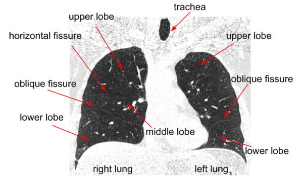
Human lungs are divided by fissures into lobes (Fig. 1). The left lung typically has 2 lobes (upper and lower) divided by one oblique fissure and the right lung typically has 3 lobes (upper, middle and lower). In healthy lungs, the major fissures typically consist of double layers of infolded invaginations of the visceral pleura. Both bronchial and vascular systems in each lobe are largely isolated with minimal connections between lobes, and the lobes can be considered as relatively independent function units. Hence, early diseases of several types may begin in and/or be confined to an individual lobe. An automated scheme for lung lobe segmentation may not only be useful for identifying and characterizing chronic diseases such as chronic obstructive pulmonary disease (COPD) and interstitial lung disease (ILD), but could also help facilitate pre-operative planning and post-operative assessments [1, 2] as well as intra-patient registration and comparison of sequential imaging procedures [3, 4]. Unfortunately, performing this task manually is extremely difficult and time consuming because of the need to mentally track and reconstruct the three-dimensional contours of pulmonary fissures that often span over multiple computed tomography (CT) images. This task is largely impractical in sub-millimeter thin-section CT examinations where hundreds of images are typically generated in each examination. Therefore, the development of a robust automated lobe segmentation scheme could be extremely beneficial for routine clinical practices and as important perhaps for quantitative lung CT image analysis.

Fig. 1.

A coronal view of the human lung as depicted on a CT examination.

Pulmonary lobe segmentation often begins with the detection of pulmonary fissures that are used as anatomical landmarks (boundaries) to separate the lobes from each other. It is well known that the fuzzy appearance of fissures on CT images, in particular in the presence of abnormalities near the fissures, makes the computer-aided detection of fissures a challenging task. Given a known fissure position (location), it is still difficult to achieve an accurate smooth segmentation of lobes because fissures depicted on CT images are frequently incomplete (Fig. 1) and commonly used algorithms (e.g., region-growing or flooding operations) may lead to a fusion of the region of interest (i.e., the lobe in question) with neighboring lobes.

Previously described lobe segmentation methods can be classified into two general categories, namely anatomy knowledge based and shape analysis based schemes. Anatomy knowledge based schemes depend on either local or global knowledge of the anatomy of lung structures. Considering the fact that there should not be any large vessels in the vicinity of pulmonary fissures, Kuhnigk et al [5] identified lobes using an interactive three-dimensional watershed algorithm. To take advantage of the linear appearance of fissures, Zhou et al. [6] and Saita et al. [7] classified the vessels and bronchi into 5 lobe regions using an edge detection method and the Hough transform based curved surface detection method, respectively. Since human lungs are similar in anatomy, Zhang et al. [8-10] developed a lobe segmentation method based on a global pulmonary atlas (template) encoded with gray level information and anatomic shape characteristics. The second class of schemes, namely shape based analysis followed by tissue classification in two- or three-dimensional image space, is somewhat different. These detection methods in the two-dimensional image space include primarily curve-growing strategies [11-12] and Vanderbrug linear feature detectors [5]. In the three-dimensional space these methods primarily include the Gaussian and mean curvature analysis approach [13] and the shape classification scheme (e.g. blobs, lines and planes classification) using an eigenvalue analysis of Hessian matrices [14]. As anatomic knowledge based schemes heavily rely on inter-examination “similarity” and largely ignore individual variability [4], these may lead to segmentation failures when the methods are applied to “new” examinations. In contrast, shape based analysis approaches in image space are often sensitive to noise or reconstruction artifacts due to the requirement for computing second derivatives of voxels’ intensity values. Although “de-noising” operations in image space (e.g. using a three-dimensional Gaussian filter [14]) are possible, filtering processes typically “broaden” the boundaries and lower the signal levels of the already weak fissure information.

On the basis of our previously developed fissure detection scheme, we present an automated lobe segmentation scheme using Radial Basis Functions (RBFs) to fit pulmonary fissure surfaces as implicit functions. The “smooth” interpolation and extrapolation enabled by the use of implicit functions allows a smooth estimation of incomplete fissures, if any, thus leading to an automatic and “natural” segmentation of lobes. The underlying assumption is that a smooth extension of fissure surfaces may be used to estimate reasonably well the “incomplete” fissures since pulmonary fissures are typically in freeform anatomic surfaces. A detailed description of the scheme and preliminary results on 65 CT examinations are described.

II. METHODS

A. Scheme Overview

The proposed automated lobe segmentation method includes three processing stages (Fig. 2): (1) lung volume segmentation, (2) fissure detection, and (3) lobe identification. The computerized schemes used in the first two stages have been described previously; therefore, the first two stages are only briefly summarized here and the majority of this paper is focused on the last stage, namely lobe identification.

Fig. 2.

Schematic diagram of the pulmonary lobe segmentation algorithm

B. Lung Volume Segmentation

To assure accurate segmentation of lung lobes, the lung itself has to be segmented appropriately. This includes adequate separation of the right and left lungs and the elimination of erroneous detection, which may lead to the inclusion of false positive identification of other organs (e.g., the liver). A large number of lung related segmentation methods have been developed for specific applications that include but are not limited to quantitative assessment of emphysema [15-16], lung nodule detection [17-19], diagnosis and quantification of interstitial lung disease [20-22], and airway analysis [23]. Many of these methods do not need to have “clean” and “complete” lung segmentation because there is little concern about possible inclusion of non-lung tissues in the analysis. Even for the purpose of fissure detection, accurate lung volume segmentation does not always have a significant effect on performance. However, for accurate lobe segmentation this is not the case. Therefore, in this study we used an automated lung segmentation approach termed Adaptive Border Marching Algorithm (ABMA) [24]. The use of this algorithm results in a “smooth” lung boundary with high computational efficiency. A detailed description of the scheme along with experimental results has been reported elsewhere [24].

C. Pulmonary Fissure Detection

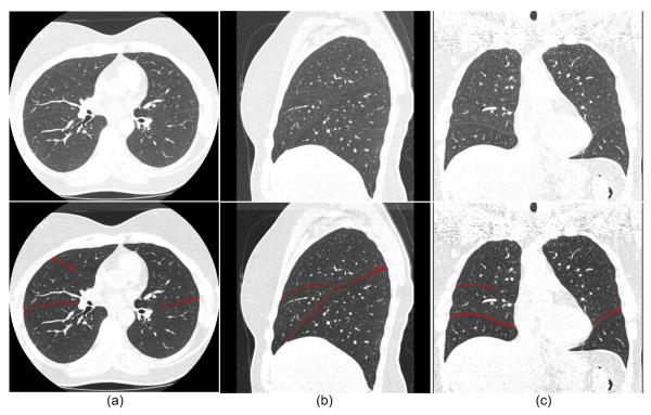
After lung segmentation, a previously developed automated scheme [25] is applied to detect pulmonary fissures by combining computational geometry approaches with statistical analysis. The underlying idea is to approximate three-dimensional freeform fissure surfaces using a set of small plane patches. In brief, the pulmonary fissure detection scheme (procedure) includes three steps (shown in Fig. 2). First, considering that the majority of pulmonary fissures are represented by higher intensity levels than parenchyma tissue and lower intensity levels than lung vessels, the scheme uses a dual threshold method (e.g., 400HU ≤ threshold ≤ 800HU) to narrow the search space for initial candidate fissure-related voxels depicted on CT images by discarding the majority of voxels related to non-fissure pulmonary tissues such as lung vessels. Second, after image thresholding, the volumetric CT image data are divided into a 3D grid structure with a set of small sub-volumes (e.g., 15×15×15 mm³) so that the fissure (if any) in each sub-volume can be approximated by a plane patch. A statistical approach based on extended Gaussian image (EGI) [26] is then applied to each sub-volume to detect depicted plane “patches” (if these exist), and the resulting plane patches are treated as initial detected fissures. Third, an “extension” procedure is performed by repeating the fissure detection procedure based on voxels contained within the initially detected fissures until there are no “plane-like” regions found. Details of this algorithm can be found elsewhere [25]. As an example, Fig. 3 shows the automated fissure detection results of the algorithm.

Fig. 3.

Examples of automated fissure detection results in an axial view (a), a coronal view (b), and a sagittal view (c). The top row shows the original images and the bottom row shows the images with an overlay of the automated fissure detection results.

D. Lobe Identification

Pulmonary fissures form the boundaries between two adjacent lobes, but it is difficult to achieve a smooth segmentation of the lobes because these fissures are often incomplete [4, 27-29] and it is extremely difficult, if not impossible, for a computerized scheme to detect all fissures depicted on CT images. Given “incomplete” fissures, typically used algorithms (e.g., region-growing or flooding operations) may lead to a fusion of neighboring lobes. As a way of “fixing” the incomplete fissures, simply extending the boundaries of the detected fissures in a linear manner to the lung boundaries using planes will lead to a non-smoothed segmentation and this approach cannot assure a reasonable estimation of incomplete fissures. To address this problem, we propose to represent the fissure surfaces in the form of smooth implicit functions using Radial Basis Functions (RBFs). The underlying motivation for this approach was to take advantage of the interpolative and extrapolative characteristics of implicit functions so that “incomplete” fissures can extend “naturally” to the lung boundaries, thus separating lung volumes into pulmonary lobes without a concern for possible fusion into neighboring lobes. There are four basic steps involved in this lobe segmentation procedure (Fig. 2).

D.1. Fissure Representation, Decomposition, and Classification

To extend detected fissures to lung boundaries properly, one needs to identify the specific fissures that may be classified as major, minor, or accessory fissure. Otherwise, it is not possible to determine where the extension procedure should terminate (e.g., the minor fissure in the right lung may penetrate the major fissure and thus divide the right lung into four different distinct segments). To achieve this goal, we represent fissures as geometric surfaces and decompose them into different patches that are then classified into major, minor, or accessory fissures using an area-based size criterion.

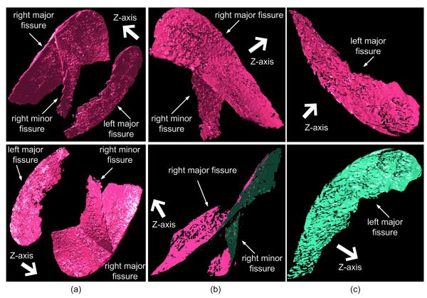
Using the Marching Cubes Algorithm (MCA) [30], the detected fissures, which are formed by discrete voxels, can be represented in the form of triangle based surfaces (Fig. 4(a)). We note that the front faces of a surface model are consistently displayed in pink while the back faces in green in this study. The MCA treats each voxel in the scalar field as a cube and determines the isosurface along each cube edge based on linear interpolation while considering the eight voxels at the corners of each cube (voxel). If a cube has one or more voxels with intensities larger than a predefined iso-value (threshold), this cube will contribute a set of triangles to the mesh. After traversing all voxels, a mesh like surface will be constructed. A detailed description of the MCA has been presented elsewhere [30]. Representation of fissures as geometric surfaces has a number of advantages. First, it provides an intuitive shape description of pulmonary fissures and fits their actual surface appearance in anatomy. Second, using this representation it is easy to compute the normal vector at any point on the assumed fissure surfaces. The computed normal vectors play an important role in the fissure decomposition and the implicit function approximation discussed later in the paper. Third, when using this representation it is possible to apply a number of well developed computational geometry techniques for specific analysis of fissures. For example, it is relatively easy to qualitatively compute (estimate) fissure completeness when fissures are represented in the form of geometric surfaces.

Fig. 4.

An example of fissure decomposition: (a) the detected fissure surfaces after modeling using the Marching Cubes Algorithm (MCA); (b) the decomposed fissure in the right lung; and (c) the decomposed fissure in the left lung. The front (top) and back (bottom) views of the modeled objects are shown. The arrow in bold in the top row of (a) indicates the Z-axis, i.e., the direction from the base of the lung to the apex.

After applying the MCA to the identified fissures, a simple approach is employed to decompose fissures by taking advantage of the relative occlusions among the different types of fissures along the z-axis (namely, the direction from the base of the lung to the apex). This can be done quite efficiently by applying a simple dot product operation. Assuming $N_i^t$ is the normal vector of the ith triangle of the fissure model, Z is the z-axis vector, and ε is a positive predetermined real value, all triangles that satisfy the condition $N_i^t\cdot Z>\epsilon$ are maintained and all other triangles are deleted / discarded. This operation has two advantages: 1) the fissures are separated into front and back surfaces and the geometric information associated with the fissure surfaces is retained; and (2) the fissures in the right lung are decomposed automatically into two patches corresponding to the “major” and the “minor” fissures (Fig. 4 (b)). The value ε in the dot product operation was set empirically to 0.3 based on experimental observations. This experiment also indicated that the performance of the scheme was insensitive to the value of ε as long as 0.25 ≤ ε ≤ 0.5. The examples in Fig. 4 (b) and (c) demonstrate the detected fissure patches after application of this operation. The major and minor fissures are separated and only their front surfaces remain, while the back surfaces are deleted / discarded. The small sparse “holes” indicate “bumpy” regions that are deleted by the dot product operation. Due to the higher curvatures of the points around the bumpy regions, a larger ε will result in larger holes because fewer triangles around the bumpy regions satisfy the condition $N_i^t\cdot Z>\epsilon$.

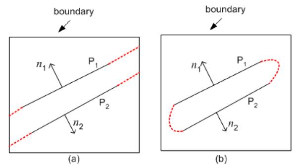
In this study, we aim to “naturally” expand computationally incomplete fissures to the lung boundary using the interpolation / extrapolation properties of implicit functions that are described in detail in the next section. To allow for an appropriate expansion we have to first decompose fissures into front-side and back-side surfaces and use only one of these surfaces for the implicit surface fitting. If we use both sides during fitting, the energy minimization based expansion, will result in rapid merging of the front and back surfaces. A simple example of this problem is presented in Fig. 5. Assuming two planes P₁ and P₂ with normal vectors n₁ and n₂, respectively, our objective is to expand these planes to the boundary surrounding the box. Fig. 5(a) shows the desired result when the surfaces are represented independently as an implicit function. Fig. 5(b) shows the results when the surfaces are not treated separately and energy minimization causes the two surfaces (P₁ and P₂) to connect / merge rather than expand to the boundary.

Fig. 5.

Expansion of two planes, namely P₁ and P₂ with normal vectors n₁ and n₂ respectively, to the boundary of a box: (a) expansion results when the two planes (P₁ and P₂) are represented separately by an implicit function; and (b) expansion results when the two planes (P₁ and P₂ ) are represented by an implicit function as a unit. The red dashed lines indicate the expansion results.

Once fissure surfaces are decomposed, the scheme identifies the type of fissures in question (i.e., major, minor, and accessory fissures) depicted in the right lung using a simple area-based size criterion. Based on this criterion, the scheme sorts the order of decomposed fissure patches in the right/left lung from the largest to the smallest in area. The first two in the sorting list related to the right lung are assigned as the major and minor fissures respectively, and the remaining fissures (if any) are considered as accessory fissures (Fig. 4). The first fissure patch in the sorting list related to the left lung is assigned as the major fissure in the left lung. The areas of the decomposed fissure patches can simply be computed by summing up the areas of the contained triangles ( mm² ). In addition, for lobe segmentation purposes, the accessory fissures are discarded.

D.2. Implicit Surface Fitting Using Radial Basis Functions

The possible existence of incomplete fissures forces us to implement an algorithm aimed to “expand” fissures to the lung boundaries. In this study, we do so by representing fissure surfaces in implicit functions. The motivation is to exploit the interpolation and extrapolation properties exhibited by an implicit function, thus estimating the missing regions of fissures in an “implicit” manner. The problem can be stated as: given a set of points in any dimensional space {x₁, x₂, …, x_n}, find a smooth function F (x) that passes through all points:

$$F\left({\mathbf{x}}_i\right)=0,i=1,2,\dots ,n$$ (1)

In our case F has a dimensionality of three due to the three-dimensional shape of the fissure surfaces, and the scattered points are all assumed to be located on the detected fissures.

There are two primary approaches to surface fitting [31-34]. One approach is an algebraic implicit surface fitting that can be represented as a polynomial (linear, quadratic, or higher) with real roots. Despite the theoretically possible high accuracy, the need for high degree polynomials frequently makes the fitting process somewhat unpredictable [33]. The other approach uses variational techniques that are based on the minimization of an energy measurement function. In the three-dimensional space, one of the simplest energy measures that can be used for this purpose can be represented as a combination of the square of the second partial derivatives along each dimension, namely:

$$\begin{array}{cc}\hfill E& =\int \int \int \left[{\left(\frac{{\partial }^{2}F}{\partial x^2}\right)}^2+{\left(\frac{{\partial }^{2}F}{\partial y^2}\right)}^2+{\left(\frac{{\partial }^{2}F}{\partial z^2}\right)}^2+{\left(\frac{{\partial }^{2}F}{\partial xy}\right)}^2+{\left(\frac{{\partial }^{2}F}{\partial xz}\right)}^2+{\left(\frac{{\partial }^{2}F}{\partial yz}\right)}^2\right]dxdydz\hfill \\ \hfill & ={\int }_{\Omega }(F_{xx}^2+F_{yy}^2+F_{zz}^2+2F_{xy}^2+2F_{xz}^2+2F_{yz}^2)d\Omega \hfill \end{array}$$ (2)

where Ω denotes a three-dimensional surface and E is a measure of the energy function in “smoothness”. Any perturbation (e.g. creases) in the surface, which is computed by second partial derivatives, would result in large changes in the computed energy. In other words, minimization of E will assure a smooth surface. As pointed out by Duchon [35], this type of energy minimization process can be solved through representation of a given surface using RBFs:

$$F\left(\mathbf{x}\right)=\sum _{i=1}^n{\lambda }_i\Phi (\mid \mathbf{x}-{\mathbf{x}}_i\mid )+P\left(\mathbf{x}\right)$$ (3)

where Φ is the RBF, λ_i are real number coefficients, P is a low degree polynomial, and { x_i } are the scattered points. For a given application, the RBFs need to be selected appropriately taking into consideration the dimensionality of the space. Several popular RBFs are listed below:

1. Φ(x) =∣x∣ (bi-harmonic or linear spline)

2. Φ(x) =∣x∣³ (tri-harmonic spline)

3. Φ(x) = e^−a∣x∣2 (Gaussian RBF)

4. Φ(x) =∣x∣² log∣x∣ (thin-plate spline)

5. $\Phi \left(\mathbf{x}\right)=\sqrt{{\mid \mathbf{x}\mid }^2+c},(c>0)$ (multi-quadric)

For example, Gaussian RBFs are primarily used in neural networks, the thin-plate spline is suitable for two-dimensional fitting problems, and the bi-harmonic and tri-harmonic splines generally work well in three-dimensional fitting problems. In this study, we used the tri-harmonic spline as the RBF in Eq. (3).

In our specific case the degree of the polynomial part in Eq. (3) should be four or lower. Otherwise, it may be difficult to control the fitting result [36]. By setting a proper constraint on the polynomial part, even in sparse datasets, appropriate shape features can be captured in the fitted surface [33]. For simplicity purposes, P(x) is often represented in a linear form for three-dimensional fitting problems:

$$P\left(\mathbf{x}\right)=\mathbf{cx}=c_0+c_{1}x+c_{2}y+c_{3}z$$ (4)

where c = (c₀,c₁,c₂,c₃).

If F passes through all scattered points { x_i }, the following condition is met:

$$F\left({\mathbf{x}}_k\right)=\sum _{i=1}^n{\lambda }_i\Phi (\mid {\mathbf{x}}_j-{\mathbf{x}}_i\mid )+P\left({\mathbf{x}}_j\right)=0$$ (5)

where j ∈ [1, n], and λ and c are unknowns. To avoid a trivial solution (i.e., λ =0 and c=0), we can sample additional points to verify that F(x) is non-zero. One simple approach is to sample off-surface points along the normal vectors of the scattered points. When an off-surface point is located on the positive/negative direction of a normal vector, it defines the “outside/inside” regions of an object. Thus, we can assign a positive/negative value to this point, namely the off-surface distance. The off-surface distance should be small enough to ensure that it does not pass through other parts of the same surface [34]. This formulation is similar to the definition of the signed distance field of an object.

Assuming a total of k off-surface points are sampled, Eq. (5) can be rewritten in a form

$$\left[\begin{array}{cccccccc}\hfill {\Phi }_{11}\hfill & \hfill {\Phi }_{12}\hfill & \hfill \cdots \hfill & \hfill {\Phi }_{1m}\hfill & \hfill 1\hfill & \hfill x_1\hfill & \hfill y_1\hfill & \hfill z_1\hfill \\ \hfill {\Phi }_{21}\hfill & \hfill {\Phi }_{22}\hfill & \hfill \cdots \hfill & \hfill {\Phi }_{2m}\hfill & \hfill 1\hfill & \hfill x_2\hfill & \hfill y_2\hfill & \hfill z_2\hfill \\ \hfill ⋮\hfill & \hfill ⋮\hfill & \hfill \hfill & \hfill ⋮\hfill & \hfill ⋮\hfill & \hfill ⋮\hfill & \hfill ⋮\hfill & \hfill ⋮\hfill \\ \hfill {\Phi }_{m1}\hfill & \hfill {\Phi }_{m2}\hfill & \hfill \cdots \hfill & \hfill {\Phi }_{mm}\hfill & \hfill 1\hfill & \hfill x_m\hfill & \hfill y_m\hfill & \hfill z_m\hfill \\ \hfill 1\hfill & \hfill 1\hfill & \hfill \cdots \hfill & \hfill 1\hfill & \hfill 0\hfill & \hfill 0\hfill & \hfill 0\hfill & \hfill 0\hfill \\ \hfill x_1\hfill & \hfill x_2\hfill & \hfill \cdots \hfill & \hfill x_m\hfill & \hfill 0\hfill & \hfill 0\hfill & \hfill 0\hfill & \hfill 0\hfill \\ \hfill y_1\hfill & \hfill y_2\hfill & \hfill \cdots \hfill & \hfill y_m\hfill & \hfill 0\hfill & \hfill 0\hfill & \hfill 0\hfill & \hfill 0\hfill \\ \hfill z_1\hfill & \hfill z_2\hfill & \hfill \cdots \hfill & \hfill z_m\hfill & \hfill 0\hfill & \hfill 0\hfill & \hfill 0\hfill & \hfill 0\hfill \end{array}\right]\left[\begin{array}{c}\hfill {\lambda }_1\hfill \\ \hfill {\lambda }_2\hfill \\ \hfill ⋮\hfill \\ \hfill {\lambda }_m\hfill \\ \hfill c_0\hfill \\ \hfill c_1\hfill \\ \hfill c_2\hfill \\ \hfill c_3\hfill \end{array}\right]=\left[\begin{array}{c}\hfill {\nu }_1\hfill \\ \hfill {\nu }_2\hfill \\ \hfill ⋮\hfill \\ \hfill {\nu }_m\hfill \\ \hfill 0\hfill \\ \hfill 0\hfill \\ \hfill 0\hfill \\ \hfill 0\hfill \end{array}\right]$$ (6)

of where Φ_ij = Φ(x_i - xj) with i, j ∈ [1, m] , m = n + k , v_i = 0 for all points located on the surface, and v_i = +1 or −1 for points located either “outside” or “inside” the surface. As a symmetric linear system, a unique non-trivial solution can be computed for Eq. (6) [37].

To demonstrate the interpolation and extrapolation properties of an implicit function based on RBFs, a general example with freeform surface is presented in Fig. 6. After the implicit function fitting of the surfaces in Fig. 6(a) and 6(c), the missing regions (or holes) are smoothly estimated (filled in) as shown in Fig. 6(b) and 6(d) correspondingly.

Fig. 6.

An example of implicit surface fitting: (a) and (c) represent original surfaces with missing regions viewed from different directions, and (b) and (d) show the interpolated/extrapolated surfaces respectively.

The detected fissures have specific associated thicknesses; hence, we assigned the mid-layer of the fissures, defined as a surface having an equal distance to the front and back surfaces of any fissure, as the separation boundary between the respected lobes. As a result, the fissures themselves are assigned equally to neighboring lobes. The mid-layer is approximated by an offset operation, which is implemented by simply moving each vertex of the front surface a small distance equal to half the minimum distance to the back surface along the opposite direction of its normal vector. In the cases where fissures need to be displayed separately along with the corresponding lobes, the previously detected fissure regions can be simply marked after lobe segmentation.

As demonstrated by Eq. (6), the linear system used to compute the implicit function is not sparse and its size is proportional to the number of the sampled (scattered) points. As a symmetric matrix, it can be reduced in size by half by storing the lower or the upper triangles only. Regardless, the storage requirement remains very large with high computational cost. As an example, 50,000 scattered points require at least 5.0GB memory as compared with the storage of the fissure surfaces modeled by the MCA that contain approximately 500,000~1,000,000 triangles corresponding to 250,000~500,000 vertices. Although we only consider here the major/minor fissure patches of right/left lung separately, the storage requirement may exceed the capability of modern PCs. To represent the fissure surfaces with high accuracy while using a substantially smaller number of sampled points, we introduce a greedy sampling scheme that consists of the following four steps:

1. Randomly select a set of vertices from the triangle mesh representing a fissure and sample the same number of off-surface points along the normal vectors of these vertices. The number of vertices should not be less than 3 due to the dimensionality of the fissure surface.

2. Reconstruct an implicit surface function using these selected vertices and off-surface constraint points as constraint points for the linear system (i.e., Eq. (6)).

3. Evaluate the error of the implicit function at each vertex on the fissure surface. If the largest error is larger than a predetermined error value ζ or accuracy, then add the vertex with the largest error and its off-surface point to the constraint point set. The error value ζ is defined as the Hausdorff distance/metric between a pair of surfaces.

4. Repeat Steps (2) and (3) until a predetermined accuracy is achieved.

Using this greedy sampling scheme we found that a substantially smaller number of points can be used in the implicit surface fitting to achieve the desired error value ζ or accuracy. During testing we were able to estimate fissure surfaces with approximately 3,000 points with a maximum allowed error of 0.1 mm. We note that both surface fitting and greedy sampling operations are performed on the triangle meshes in geometric space. Hence, the fitting error is not limited by the actual CT image resolution.

D.3. Lung Lobe Identification

As the major and minor fissures are now represented in the form of implicit functions, we divide the lung volume into lobes using these implicit functions. The spatial position (x_i, y_i, z_i) of each of the voxels within the right and left lungs is checked against the implicit function representing the major respective fissure. First, the right lung volume is divided into two semi-volumes according to the positive/negative sign of each voxel with respect to the implicit function of the major fissure. Then an arbitrary point located on the minor fissure in the right lung is selected and checked against the implicit function of the major fissure. If the value is positive (or negative), the positive (or negative) semi-volume is further divided using a similar process to check each of the voxels within this semi-volume against the implicit function of the minor fissure. Thus, the right lung volume is divided into three parts and similarly, the left lung volume is divided into two semi-volumes.

III. EXPERIMENTS AND RESULTS

A. Testing CT Dataset

In a preliminary study to subjectively assess the quality of our automated lung lobe segmentation scheme we selected a dataset of 65 chest CT examinations acquired on 65 participants in a chronic obstructive pulmonary disease (COPD) screening study at the University of Pittsburgh Medical Center. These CT examinations were performed under an Institutional Review Board (IRB) approved protocol using a LightSpeed VCT 64-detector scanner (GE Healthcare, Waukesha, WI) with subjects holding their breath at end inspiration. CT data were acquired using a helical technique at a pitch of 0.969, 120 kVp, 0.4 sec gantry rotation, and 250 mA (100 mAs). The detector configuration was 32 × 0.625 mm. CT images were reconstructed to encompass the entire lung field using the GE “bone” kernel at 0.625 mm section thickness and 0.625 mm interval (without slice overlapping). The CT images were represented using a 512 × 512 pixel matrix with a pixel dimension ranging from 0.549 to 0.738 mm. To investigate the impact of CT image slice thickness on the performance of our lobe segmentation scheme, we performed two additional reconstructions for 5 of these 65 CT examinations both using the “bone” kernel: (1) 1.25 mm section thicknesses with a 1.25 mm interval and (2) 2.5 mm section thickness with a 2.5 mm interval. All subjects had relatively low levels of airflow obstruction or visually depicted emphysema on their CT examinations. Pulmonary function tests (PFT) were performed post bronchodilator using body plethysmography (Vmax 229 AutoBox, SensorMedics, Yoba Linda, CA). The mean percent predicted of forced expiratory volume in one second (FEV₁%) and forced vital capacity (FVC%) across the 65 subjects were 84.8 (±23.6) and 95.0 (±16.5), respectively.

B. Subjective Evaluation by Observers

It is extremely time consuming and in reality virtually impossible to manually segment lobes accurately through “tracing” hundreds of CT image slices in each examination and then use the manual segmentation results as a gold standard for evaluation purpose. Therefore, a direct subjective evaluation based on radiologists’ visual assessment was conducted in this study. The maximum error associated with the implicit function fitting of fissure surfaces was set at 0.1 mm for all examinations tested. We emphasize that since this fitting error is actually performed on mesh surfaces in geometric space, it is not limited by the spatial resolution of CT images after the MCA is applied. Hence, the previous qualitative assessment of our computerized fissure segmentation scheme [25] may be regarded as supporting data to be the assessment of lobe segmentation we report here. In this study, two chest radiologists (with experience of reading and interpreting chest radiographs for 28 and 15 years, respectively) were asked to independently review and subjectively rate each CT examination on a five category scale (i.e., excellent, good, fair, poor and unacceptable) to assess the quality of the computerized lobe segmentation or automated “assignment” results. During this rating process, radiologists scanned and viewed each CT examination in axial, coronal, and sagittal views. They were told that our purpose was to completely automatically segment CT examinations and provide lobar based quantitative analyses and therefore they should be critical in terms of their subjective assessment as to whether the segmentation is correct, complete, and adequate for this purpose. Since five CT examinations had been reconstructed three times with slice thicknesses of 0.625 mm, 1.25 mm and 2.5 mm and the other 60 examinations were reconstructed only once with a slice thickness of 0.625 mm, each radiologist rated a total of 75 sets of reconstructed and displayed CT examinations. Inter-reader agreement was estimated using the Weighted Kappa coefficient (PROC FREQ, SAS v.9.1.3) with significance determined by the asymptotic test under the null hypothesis that Kappa equals zero at α = 0.05 using a two-sided test.

C. Experimental Results

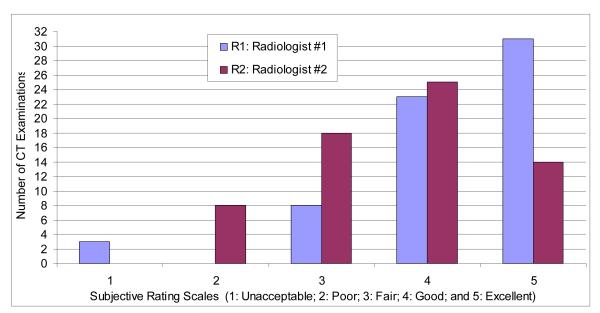
Fig. 7 summarizes the subjective performance ratings of our automated lobe segmentation scheme by the two radiologists using 65 CT examinations with a section thickness of 0.625 mm. Radiologist #1 (R1) rated 31 cases excellent, 23 good, 8 fair, and 3 unacceptable, while Radiologist #2 (R2) rated 14 examinations as excellent, 25 as good, 18 as fair, and 8 as poor. Averaging over the two readers, 50.8% (33 of 65) of the CT examinations were rated as good or better by both radiologists and only 1.5% (1 of 65) of the CT examinations was rated by both radiologists as either poor or unacceptable. Weighted Kappa was 0.1299 with a 95% confidence interval of −0.0148, 0.2746 (p = 0.0761), namely the agreement between the readers was not statistically significant.

Fig. 7.

Subjective evaluations of the computerized lobe segmentation as rated by the two radiologists (R1 and R2) on 65 CT examinations reconstructed with a section thickness of 0.625 mm.

Table 1 lists the ratings of the two radiologists for the 5 CT examinations that had been reconstructed three times with section thicknesses of 0.625 mm, 1.25 mm, and 2.5 mm. The results shown are reasonably comparable for examinations reconstructed with a section thickness of either 0.625 mm or 1.25 mm. For example, in case #3 radiologist #1 (R1) rated the examinations with a section thickness of 0.625 mm and 1.25 mm as “excellent” and “fair”, respectively, and in cases #1 and #2 radiologist #1 (R1) rated the examinations with a section thickness of 1.25 mm as “excellent”, but the examination with a section thickness of 0.625 mm as “fair”. A similar observation can also be found in the ratings provided by radiologist #2 (R2). However, the results show that no examination reconstructed with a section thickness of 2.5 mm was rated higher than those reconstructed with a section thickness of either 0.625 mm or 1.25 mm. Thus, in general, the segmentation in the CT examinations reconstructed with 2.5 mm slice thickness was largely rated as inferior to that in the corresponding examinations reconstructed with thinner slice thicknesses.

Table 1.

Subjective ratings of the computerized lobe segmentation by two radiologists (R1 and R2) of 5 CT examinations reconstructed three times with section thicknesses of 0.625 mm, 1.25 mm, and 2.5 mm.

Case	Section Thickness	Excellent		Good		Fair		Poor		Unacceptable
		R1	R2	R1	R2	R1	R2	R1	R2	R1	R2
1	0.625 mm				X	X
	1.25 mm	X					X
	2.5 mm					X			X
2	0.625 mm					X	X
	1.25 mm	X			X
	2.5 mm					X	X
3	0.625 mm	X					X
	1.25 mm					X			X
	2.5mm							X	X
4	0.625 mm						X			X
	1.25 mm						X			X
	2.5 mm								X	X
5	0.625 mm								X	X
	1.25 mm								X	X
	2.5 mm									X	X

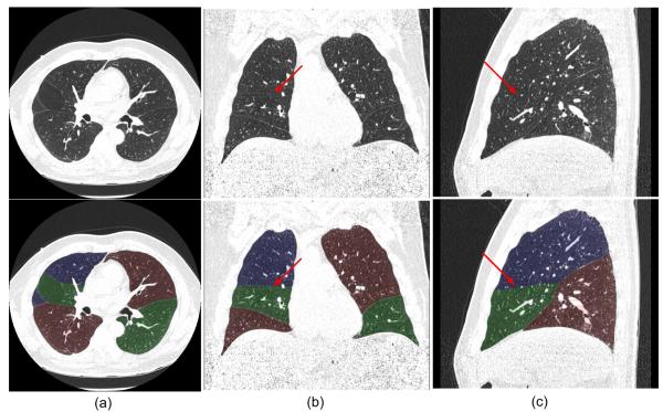
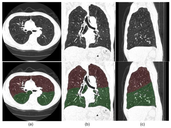
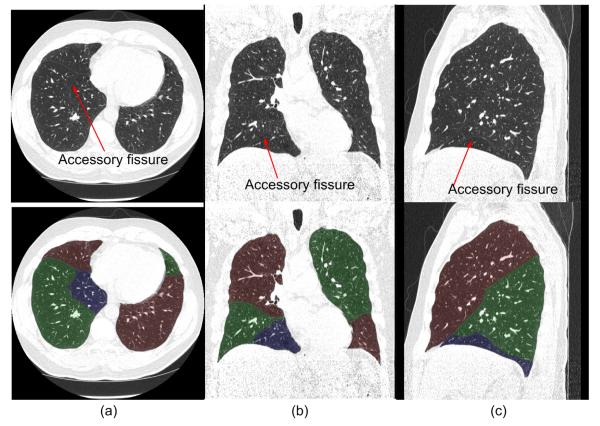
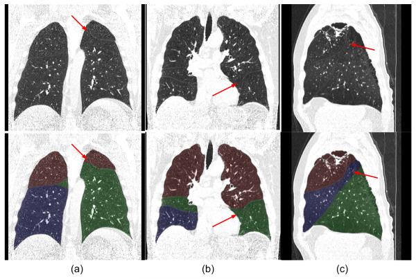
Fig. 8 shows an examination in which the “incomplete” fissures are smoothly estimated and the case was rated as “excellent” by both radiologists. Fig. 9 and 10 show two examinations rated by radiologist #2 as “unacceptable.” Among these, in one examination (as shown in Fig. 9), the middle lobe of the right lung is not segmented due to the failure in detecting the corresponding fissure surface that has extremely low contrast in the relevant CT images; while in another examination (as shown in Fig. 10), a lobe segmentation error was introduced by the detection of an accessory fissure that was misclassified as the minor fissure in the right lung. Fig. 11 shows images of three CT examinations in which the computerized lobe segmentations were rated by at least one radiologist as “good”, “fair” and “poor”, respectively. In these three examples (Fig. 11), our scheme did not detect a small fraction of fissures near the lung boundaries and as a result the fissure fitting results in a small deviation (offset) from the actual fissures.

Fig. 8.

An example of an examination with an incomplete fissure that was rated as “excellent” for lobe segmentation with the axial view (a), coronal view (b), and sagittal view (c) shown. The original images (top) and the images with transparent overlays of the automated lobe segmentation (bottom) are shown. The arrows indicate the positions where fissures are not depicted on CT images.

Fig. 9.

An examination rated as “unacceptable” for lobe segmentation in which the middle lobe was not detected. Axial view (a), coronal view (b) and sagittal view (c) are shown. The original images (top) and the images with transparent overlay of the automated lobe segmentation (bottom) are shown.

Fig. 10.

An examination rated as “unacceptable for lobe segmentation” in which the accessory fissure was assigned as a minor fissure in the right lung. Axial view (a), coronal view (b) and sagittal view (c), are shown. The original images (top) and the images with transparent overlay of the automated lobe segmentation (bottom) are shown.

Fig. 11.

Three examples of examinations rated by the radiologists as “good” (a), “fair” (b), and “poor” (c) for segmentation.

IV. DISCUSSION

We introduced an automated scheme for lung lobe segmentation, which has a number of unique characteristics. First, the scheme is largely independent of the knowledge of lung anatomy that varies quite a bit among patients. It depends on but rudimentary underlying assumptions such as the fact that fissure can be represented as three dimensional continuous surfaces. Second, unlike previous shape analysis based approaches that work in image space [11-13], the proposed segmentation procedure is performed in geometric space on the basis of a statistical fissure detection approach. Similar to the fissure detection approach, the scheme is less affected by conventional image (pixel-based) noise/artifacts in the spatial domain. It is also relatively easy to implement. Third, the implicit function based representation of fissure surfaces provides a smooth estimation of incomplete fissures, thus leading to a reasonably “natural” segmentation of lung volumes into lobes. Due to the relatively high prevalence of incomplete fissures and the possible importance of assessing fissure completeness in clinical practice [27-29], the proposed method may be used to assess fissure incompleteness in a quantitative manner. Fourth, the geometric characteristic of this scheme allows for a three-dimensional visualization of human lung anatomy. Hence, it enables both regional and local quantitative analyses to be performed. Finally, the capability of our approaches in segmenting fissures and lobes separately may provide a better understanding of lung anatomy and its correlation to lung function by building a computational model of fissure configuration and integrity. This may lead to earlier detection and diagnosis and possibly to more efficacious individualized patient management.

Although our scheme is able to detect accessory fissures, these accessory fissures do not indicate the presence of additional lobes. When an accessory fissure is larger in area than the minor fissure, the automated approach may lead to misclassification of regions as shown in Fig. 10, where the accessory fissure is misclassified as the minor fissure due to the use of our area-based fissure type classification criterion. As the fissures cannot always be fully and accurately detected by computerized schemes due to their fuzzy appearance and possible anatomical incompleteness, the reconstructed implicit function may cause obvious fissure extension errors as shown in Fig. 9 and Fig. 11. More robust approaches to solve this problem are currently under investigation.

Despite the fact that mathematically implicit surface fitting based on RBFs is a very reliable procedure for interpolation/extrapolation purposes, the fitting accuracy between the reconstruction implicit functions and the actual fissure surface in this study is largely determined by the number of sampling points. A greedy sampling strategy can adaptively select the “most important” points hence help overcome some of the limitations of computer memory. The original fissure surfaces are not perfectly “smooth;” therefore, neighboring “off-surface” sampled points may have normal vectors that vary greatly. In practice, a sparse and uneven normal vector property of the sampling points may lead to a rugged reconstructed surface because the mathematical property of the implicit function has to guarantee a smooth transition between neighboring sampling points. Adding sampling points could alleviate this problem somewhat, albeit at a heavier computational cost. For a typical CT examination consisting of 300~600 image slices (with a slice thickness of 0.625 mm ~ 1.25 mm), it takes approximately 25 minutes to execute our scheme on a desktop PC (installed with an AMD Athlon™ 64×2 Dual 2.11GHz central processor and 2GB RAM). Thus, improving efficiency remains an important issue that is currently under investigation.

We recognize that although CT images reconstructed with a section thickness of 0.625 mm have been available, the majority of CT image examinations used in routine clinical practice are reconstructed using lower resolution image slices (i.e., 1.25 mm or 2.5 mm) for a variety of clinical and cost reasons. Thus, in this study we investigated the performance dependence of our scheme on CT image slice thickness. Our experimental results showed that there was no observable difference in radiologists’ subjectively acceptance rating levels when applying our scheme to CT examinations reconstructed with a section thickness of either 0.625 mm or 1.25 mm. Generally, fissures depicted on CT images reconstructed with a section thickness of 0.625 mm have a little bit higher contrast but much smaller thickness (which means fewer information of fissures) than those on CT images with a section thickness of 1.25 mm. Such a fact occasionally leads to a more robust detection of fissures depicted on CT images with a section thickness of 0.625 mm. As a result, a radiologist may rate higher acceptance levels to some CT examinations reconstructed with a section thickness of 0.625 mm and other examinations with a section thickness of 1.25 mm. However, when the slice thickness increases to 2.5 mm, our visual observation found that the contrast of fissures decreased dramatically, thus making the segmentation performance unpredictable.

Only 33 of the 65 examinations (50.8%) evaluated in this study that had a section thickness of 0.625 mm were rated by both radiologists as either “good” or “excellent” in terms of segmentation quality. This does not mean that the scheme failed to segment other examinations. As demonstrated in Fig. 10 and Fig. 11, the radiologists rated the lobe segmentation performance primarily based on local failures / errors. The majority of the lobes were segmented successfully even in those examinations subjectively rated as “unacceptable”. This may be the very reason why only one case (1.5%) was rated by both radiologists as “poor” and /or “unacceptable”. We found out that lobe segmentation errors were directly proportional to the fraction of incompleteness of the computed (estimated) fissures. Previous studies [27-29] demonstrated that over 40% of the subjects have visually incomplete fissures on CT examinations. Similarly, in our study, the examinations in which segmentations were rated poorly are primarily those in which fissure incompleteness was prevalent. In the future, we will explore different approaches, including but not limited to, increasing the underlying lung anatomy based assumptions in an attempt to improve lobe segmentation performance.

In the absence of a verified “ground-truth”, absolute performance assessments of a computerized scheme are virtually impossible [38-39]. In the case of lobe segmentation, this problem is magnified because manually drawing lobe boundaries over hundreds of slices per examination is an extremely labor intensive task and one can expect substantially large inter-reader variability. In this study, lobe segmentation error was largely determined by the accuracy of fissure detection that had been assessed quantitatively in a previous study [25]. When the radiologists’ markings were used as a reference, approximately 95% of the fissure points detected by the scheme were less than 2 mm away from the fissures marked manually by the radiologists. The root mean square (RMS) distances between fissures marked by one radiologist and our scheme ranged from 1.48±0.92 mm to 2.04±3.88 mm and were smaller than the RMS distances between the two radiologists (3.34±4.98 mm and 2.64±2.76 mm). Hence, in this preliminary study we resorted to a subjective assessment method to evaluate radiologists’ ratings of the automated lung lobe segmentation results. Despite these limitations the results of this preliminary study are encouraging.

We recognized that a major limitation of this study was the lack of validation of the approach using CT examinations depicting severe lung disease (e.g., nodules/tumors, severe emphysema, fibrosis, scarring, and atelectasis). At this stage of development, our testing dataset only included CT examinations acquired from relatively healthy or mildly diseased lungs. Based on the unique characteristics of our fissure detection and surface fitting schemes, we believe that the variety of lung disease patterns may have limited impact on the lobe segmentation results because only planar tissues in the lungs are detected as potential fissures and the performance of lobe segmentation relies directly on the performance of fissure detection. However, testing of severely diseased lungs should be done and it is the topic of current effort. There are two categories of errors in fissure detection, namely false negative detection where fissures are not fully detected due to their “incompleteness” or extreme fuzzy appearance and false positive detection where tissues with plane like structures are incorrectly detected and identified as fissures (e.g., interstitial lung diseases or accessory fissures). The interpolation/extrapolation nature of the proposed scheme often results in an automated correction of the first error type. However, when a fissure is not fully detected and has a large estimated area, the surface fitting operation may estimate “incomplete” fissures incorrectly through the extrapolation operation (Fig. 11). When an incorrectly detected fissure has a small area as compared with the minor fissure, the second type of detection error does not present a problem to the lobe segmentation procedure because the area-based size criterion frequently filters out the misclassified non-fissure tissue. Otherwise, the misclassified tissue may be incorrectly assigned as a minor fissure resulting in incorrect lobe segmentation. These errors may occur more frequently in CT examinations of severely diseased lungs.

V. CONCLUSION

A new fully automated lung lobe segmentation scheme based on implicit function fitting of fissure surfaces was developed and tested. The interpolate/extrapolate properties of the RBF implicit function allows for a smooth estimation of incomplete fissures and offers a unified framework for similar problems. Subjective assessments by two experienced radiologists showed that 50.8% (33/65) of the CT examinations with a section thickness of 0.625 mm were rated as either “excellent” or “good” by both radiologists and only 1.5% (1/65) was rated by both radiologists as “poor” or “unacceptable”. We note the large inter-reader variability is a well-known phenomenon in subjective rating studies. The computerized scheme did not work well with CT examinations having a section thickness of 2.5 mm. The procedures involved in this scheme are performed in three-dimensional geometric space and the resulting representation of the segmented lung may ultimately enable automated segmentation and quantitative lung CT image analysis.

REFERENCES

- [1].Modgil V, Das S, Suri R. Anomalous Lobar Pattern of Right Lung: A Case Report. International Journal of Morphology. 2006;Vol. 24(1):506–507. [Google Scholar]
- [2].Venuta F, Rendina EA, Giacomo TD, Flaishman I, Guarino E, Ciccone AM, Ricci C. Technique to Reduce Air Leaks after Pulmonary Lobectomy. 1998;Vol. 3(4):361–364. doi: 10.1016/s1010-7940(98)00038-4. [DOI] [PubMed] [Google Scholar]
- [3].Sluimer I, Schilham A, Prokop M, van Ginneken B. Computer Analysis of Computed Tomography Scans of the Pulmonary: A Survey. IEEE Trans. Medical Imaging. 2006;Vol. 25(4):385–405. doi: 10.1109/TMI.2005.862753. [DOI] [PubMed] [Google Scholar]
- [4].Hayashi K, Aziz A, Ashizawa K, Hayashi H, Nagaoki K, Otsuji H. Radiographic and CT Appearances of the Major Fissures. Radiographics. 2001;Vol. 21(4):861–874. doi: 10.1148/radiographics.21.4.g01jl24861. [DOI] [PubMed] [Google Scholar]
- [5].Kuhnigk JM, Hahn H, Hindennach M, Dicken V, Krass S, Peitgen HO. Pulmonary Lobe Segmentation by Anatomy-Guided Three-dimensional Watershed Transform. Proceedings of SPIE (Medical Imaging).2003. pp. 1482–1490. [Google Scholar]
- [6].Zhou X, Hayashi T, Hara T, Fujita H, Yokoyama R, Kiryu T, Hoshi H. Automatic Recognition of Pulmonary Lobes and Fissures from Multi-slice CT Images. Proceeding of SPIE (Medical Imaging).2004. pp. 1629–1633. [Google Scholar]
- [7].Saita S, Kubo M, Kawata Y, Niki N, Ohmatsu H, Moriyama N. An Algorithm for the Extraction of Pulmonary Fissures from Low-dose Multislice CT Image. System and Computers in Japan. 2006;Vol. 37(9):63–76. [Google Scholar]
- [8].Zhang L, Hoffman EA, Reinhardt JM. Pulmonary Lobe Segmentation by Graph Search with 3-D Shape Constraints. Proceedings of SPIE (Medical Imaging).2001. pp. 204–215. [Google Scholar]
- [9].Zhang L, Reinhardt JM. Detection of Pulmonary Lobar Fissures using Fuzzy Logic. Proceedings of SPIE (Medical Imaging).1999. pp. 188–199. [Google Scholar]
- [10].Zhang L, Hoffman EA, Reinhardt JM. Atlas-driven Pulmonary Lobe Segmentation in Volumetric X-ray CT Images. IEEE Trans. Medical Imaging. 2006;Vol. 25(1):1–16. doi: 10.1109/TMI.2005.859209. [DOI] [PubMed] [Google Scholar]
- [11].Wang J, Betke M, Ko JP. Pulmonary Fissure Segmentation on CT. Medical Image Analysis. 2006;Vol. 10:530–547. doi: 10.1016/j.media.2006.05.003. [DOI] [PMC free article] [PubMed] [Google Scholar]
- [12].Wang J, Betke M, Ko JP. Lecture Notes in Computer Science. Vol. 3216. Springer-Verlag; Berlin, Germany: 2003. Shape-based Curve Growing Model and Adaptive Regularization for Pulmonary Fissure Segmentation in CT; pp. 541–548. Medical Image Computing and Computer-Assisted Intervention. [Google Scholar]
- [13].Kubo M, Kawata Y, Niki N, Eguchi K, Ohmatsu H, Kakinuma R, Kaneko M, Kusumoto M, Moriyama N, Mori K, Nishiyama H. Automatic Extraction of Pulmonary Fissures from Multidetector-row CT Images. Proceedings of the IEEE International Conference on Image Processing (ICIP’01); Greece. 2001. pp. 1091–1094. [Google Scholar]
- [14].Kitasaka T, Nakada Y, Mori K, Suenaga Y, Mori M, Takabatake H, Natori H. Recognition of Lung Lobes and its Application to the Bronchial Structure Analysis. Proceedings of the 18th International Conference on Pattern Recognition (ICPR’06).2006. pp. 288–291. [Google Scholar]
- [15].Lukose R, Paul S, Sunitha, Daniel M, Abraham SM, Abraham, Alex ME, Thomas R, Nair V, Abraham SM, Alex ME. Morphology of the Lungs: Variations in the Lobes and Fissures. Biomedicine. 1999;Vol. 19(3):227–232. [Google Scholar]
- [16].Ariyürek MO, Karabulut N, Yelgeç SN, Gülsün M. Anatomy of the Minor Fissure: Assessment with High-resolution CT and Classification. European Radiology. 2004;Vol. 12(1):175–180. doi: 10.1007/s003300100907. [DOI] [PubMed] [Google Scholar]
- [17].Bae KT, Kim JS, Na YH, Kim KG, Kim JH. Pulmonary Nodules: Automated Detection on CT Images with Morphologic Matching Algorithm—Preliminary Results. Radiology. 2005;Vol. 236:286–294. doi: 10.1148/radiol.2361041286. [DOI] [PubMed] [Google Scholar]
- [18].Lee Y, Hara T, Fujita H, Itoh S, Ishigaki T. Automated Detection of Pulmonary Nodules in Helical CT Images Based on an Improved Template-Matching Technique. IEEE Trans. Medical Imaging. 2001;Vol. 20(7):595–604. doi: 10.1109/42.932744. [DOI] [PubMed] [Google Scholar]
- [19].Rubin GD, Lyo J, Paik DS, Sherbondy A, Chow L, Leung AN, Mindelzun R, Zinck SE, Naidich DP, Napel S. Pulmonary Nodules in MDCT Scans: Impact of Computer-aided Detection. Radiology. 2005;Vol. 234:274–283. doi: 10.1148/radiol.2341040589. [DOI] [PubMed] [Google Scholar]
- [20].Brown MS, McNitt-Gray MF, Goldin JG, Suh RD, Sayre JW, Aberle DR. Patient-Specific Models for Lung Nodule Detection and Surveillance in CT Images. IEEE Trans. Medical Imaging. 2001;Vol. 20(12):1242–1250. doi: 10.1109/42.974919. [DOI] [PubMed] [Google Scholar]
- [21].Li Q, Katsuragawa S, Doi K. Computer Aided Diagnostic Scheme for Lung Nodule Detection in Digital Chest Radiographs by Use of a Multiple-Template Matching Technique. Medical Physics. 2001;Vol. 28(10):2070–2076. doi: 10.1118/1.1406517. [DOI] [PubMed] [Google Scholar]
- [22].Armato SG, III, Giger MI, Moran CJ, Blackburn JT, Doi K, MacMabon H. Computerized Detection of Pulmonary Nodules on CT Scans. Radiographics. 1999;Vol. 19:1303–1311. doi: 10.1148/radiographics.19.5.g99se181303. [DOI] [PubMed] [Google Scholar]
- [23].Park W, Hoffman E, Sonka M. Segmentation of Intrathoracic Airway Trees: A Fuzzy Logic Approach. IEEE Trans. on Medical Imaging. 1998;Vol. 17(4):489–497. doi: 10.1109/42.730394. [DOI] [PubMed] [Google Scholar]
- [24].Pu J, Roos J, Yi CA, Napel S, Rubin GD, Paik DS. Adaptive Border Marching Algorithm: Automatic Lung Segmentation on Chest CT Images. Computerized Medical Imaging and Graphics. 2008;Vol. 32(6):452–462. doi: 10.1016/j.compmedimag.2008.04.005. [DOI] [PMC free article] [PubMed] [Google Scholar]
- [25].Pu J, Leader JK, Zheng B, Knollmann F, Fuhrman C, Sciurba FC, Gur D. A Computational Geometry Approach to Automated Pulmonary Fissure Segmentation in CT Examinations. IEEE Trans on Medical Imaging. 2009;Vol. 28(5):710–719. doi: 10.1109/TMI.2008.2010441. [DOI] [PMC free article] [PubMed] [Google Scholar]
- [26].Horn B. Proc. IEEE 72. 12. Vol. 12. New Orleans, USA: 1984. Extended Gaussian Images; pp. 1671–1686. [Google Scholar]
- [27].Berkmen T, Berkmen YM, Austin JHM. Accessory Fissures of the Upper Lobe of the Left Lung: CT and Plain Film Appearance. American Journal of Roentgenology. 1994;Vol. 162:1287–1293. doi: 10.2214/ajr.162.6.8191982. [DOI] [PubMed] [Google Scholar]
- [28].Mahmut M, Nishitani H. Evaluation of Pulmonary Lobe Variations Using Multi-detector Row Computed Tomography. Journal of Computer Assisted Tomography. 2007;Vol. 31(6):956–960. doi: 10.1097/rct.0b013e3180500d23. [DOI] [PubMed] [Google Scholar]
- [29].Aziz A, Ashizawa K, Nagaoki K, Hayashi K. High Resolution CT Anatomy of the Pulmonary Fissures. Thoracic Imaging. 2004;Vol. 19(3):186–191. doi: 10.1097/01.rti.0000131590.74658.24. [DOI] [PubMed] [Google Scholar]
- [30].Lorensen WE, Cline HE. Marching Cubes: A High Resolution Three-dimensional Surface Construction Algorithm. Computer Graphics. 1987;Vol. 21(4):163–169. [Google Scholar]
- [31].Bajaj C, Ihm I, Warren J. Higher-Order Interpolation and Least-Squares Approximation Using Implicit Algebraic Surfaces. ACM Trans. Graphics. 1993;Vol. 12(4):327–347. [Google Scholar]
- [32].Keren D, Gotsman C. Fitting Curves and Surfaces with Constrained Implicit Polynomials. IEEE Trans. Pattern Analysis and Machine Intelligence. 1999;Vol. 21(1):31–41. [Google Scholar]
- [33].Li Q, Wills D, Phillips R, Viant WJ, Griffiths JG, Ward J. Implicit Fitting Using Radial Basis Functions with Ellipsoid Constraint. Computer Graphics Forum. 2004;Vol. 23(1):55–69. [Google Scholar]
- [34].Carr JC, Beatson RK, Cherrie JB, Mitchell TJ, Fright WR, McCallum BC, Evans TR. ACM SIGGRAPH 2001. Los Angeles, CA: 2001. Reconstruction and Representation of 3D Objects with Radial Basis Functions; pp. 67–76. [Google Scholar]
- [35].Duchon J. Splines Minimizing Rotation-Invariant Semi-Norms in Sobolev Spaces. In: Dolb A, Eckmann B, editors. Constructive Theory of Functions of Several Variable, Lecture Notes in Mathematics. Springer-Verlag; 1977. pp. 85–100. [Google Scholar]
- [36].Keren D, Cooper D, Subrahmonia J. Describing Complicated Objects by Implicit Polynomials. IEEE Trans. Pattern Analysis and Machine Intelligence. 1994;Vol. 16(1):38–53. [Google Scholar]
- [37].Turk G, O’Brien JF. ACM SIGGRAPH 1999. Los Angeles, CA: 1999. Shape Transformation Using Variational Implicit Functions; pp. 335–342. [Google Scholar]
- [38].Chalana V, Kim Y. A Methodology for Evaluation of Boundary Detection Algorithms on Medical Images. IEEE Trans. Medical Imaging. 1997;Vol. 16(5):642–652. doi: 10.1109/42.640755. [DOI] [PubMed] [Google Scholar]
- [39].Zhang YJ. A Survey on Evaluation Methods for Image Segmentation. Pattern Recognition. 1996;Vol. 29:1335–1346. [Google Scholar]