Cryomesh™: A new substrate for cryo-electron microscopy

Abstract

Here we evaluate a new grid substrate developed by ProtoChips Inc. for cryo-transmission electron microscopy. The new grids are fabricated from doped silicon carbide using processes adapted from the semi-conductor industry. A major motivating purpose in the development of these grids was to increase the low-temperature conductivity of the substrate, a characteristic that is thought to affect the appearance of beam-induced movement (BIM) in TEM images of biological specimens. BIM degrades the quality of data, and is especially severe when frozen biological specimens are tilted in the microscope. Our results show that this new substrate does indeed have a significant impact on reducing the appearance and severity of beam-induced movement in TEM images of tilted cryo-preserved samples. Furthermore, while we have not been able to ascertain the exact causes underlying the BIM phenomenon, we have evidence that the rigidity and flatness of these grids may play a major role in its reduction. This improvement in the reliability of imaging at tilt has a significant impact on using data collection methods such as random conical tilt or orthogonal tilt reconstruction with cryo-preserved samples. Reduction in BIM also has the potential for improving the resolution of 3D cryo-reconstructions in general.

1. Introduction

‘Beam-Induced Motion’, or BIM, is a phenomenon believed to cause a range of defects that are sometimes observed in TEM images of biological samples. These same imaging defects are also commonly referred to as ‘charging’, though the two terms are not entirely synonymous. In the process of charging, illumination from the electron beam causes the release of secondary electrons from the sample, and if the sample is electrically insulating, a build-up of positive charge within that sample. This charge build-up is thought to be the cause of imaging defects such as BIM, but does not inevitably lead to them. One model holds that this static charge can act as a lens that assists, or even deflects the electron beam (Glaeser and Downing, 2004). In this model it is easy to hypothesize that if this ‘lens’ were not uniform (i.e. the static charge were not evenly distributed within the sample), or if the charge was dynamic (for example, during the initial build-up), then the resulting deflections of the beam would be similarly non-uniform and the image distorted. A second model posits that an uneven charge distribution may cause mechanical rippling motions in the sample as the increasing charge creates internal electrostatic forces (Glaeser, 2008). These forces may exploit pre-existing structural irregularities in the sample in an attempt to distribute themselves more evenly. Such structural irregularities may also increase the likelihood of uneven charge distributions, as curved surfaces are expected to accumulate charge more quickly than flat surfaces. This was demonstrated by the observation that highly curved ice droplets were more sensitive to electron dose-rates than flat ice (Chen et al., 2008).

The evidence available suggests that both models may co-exist since the list of observations attributed to ‘charging’ are diverse, and the natures of the samples being imaged (rigidity, conductivity, etc.) would have a large effect on which model was more likely to be dominant. Some of these observations include: increases in beam diameter when moving from conductive sample areas to insulating ones (Brink et al., 1998), irregular image blurring in normal imaging modes (Bottcher, 1995), blurring and deformation of diffraction spots in diffraction mode (Henderson, 1992), residual “footprints” that can be observed in the wake of imaging (called the Berriman effect) (Brink et al., 1998), and large reductions in the quality of imaged crystals when compared to their electron diffraction patterns (Henderson and Glaeser, 1985). Of these observations, irregular image blurring best corresponds with BIM as discussed in this manuscript (see Figure 4), although some of the other observations, i.e. diffraction blurring/attenuation, may result from the same physical process. It is also important to note that there are large differences in the severity of image degradation attributed to BIM. In the case of crystal diffraction, where the quality of high-resolution data can be assessed directly, the loss of high-resolution information can be attributed to BIM though its effects may not be obvious in the actual image. In other cases, BIM can be so severe that it may make it impossible to differentiate between individual particles in a single-particle image. In this case BIM would not only limit the resolution attainable, but also the ability to perform even initial processing of the data.

Figure 4.

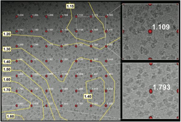
Example of a 4096² pixel CCD image at 50,000X and 45° tilt exhibiting BIM. This image would have been marked as bad in the manual evaluation even though only a small region in the lower left corner is clearly showing BIM. In this image the power spectrum peaks that were used in the computer evaluation are shown in red, centered over the 1024² pixel areas from which they were calculated. Next to each peak in white text is the computed score assigned to that region. The yellow contour lines were generated using Matlab, each encloses an image area with BIM greater than or equal to the shown score (found using interpolation). On the right, the lowest and highest scoring regions from the image are expanded for clearer visibility.

There are two situations, in particular, which can greatly increase the severity of BIM in images. The first is imaging samples that are electrically insulating, which in the case of biological materials, most acutely affects the use of cryo-preservation, a method in which biological samples are preserved in a layer of vitrified ice (Dubochet and Lepault, 1984). Cryo-preservation allows researchers to more accurately capture the biologically relevant state of specimens and to collect data at higher resolution. Unfortunately, cryo-preserved samples are more prone to BIM and are also more radiation sensitive, limiting the options available for mitigating BIM. Another problematic circumstance is imaging specimens that are tilted in the microscope. Some methods, such as electron tomography (Downing et al., 2007), electron crystallography (Glaeser, 1985), random conical tilt (RCT) (Radermacher, 1988), and orthogonal tilt reconstruction (OTR) (Leschziner and Nogales, 2006) require the collection of tilted data. Of particular interest here, RCT and OTR allow investigators to process single-particle datasets in ways that ease the study of conformationally variable or uncharacterized complexes. Unfortunately, when a sample is tilted in the microscope the specimen plane becomes less perpendicular to the electron beam and much more prone to BIM. It is theorized that this is because ‘up-and-down’ components of BIM that might have previously gone unnoticed become more harmful ‘side-to-side’ motions.

Cryo-preservation and tilted data collection rarely suffer from noticeable BIM when used alone (though BIM may still be damaging high-resolution information). Under tilted cryo conditions, however, it is our experience, and the experience of others (Rhinow and Kühlbrandt, 2008), that even in the best of cases as much as 80% of images show severe BIM. Despite the possibilities offered by combining cryo-preservation with tilted data collection, this high incidence of BIM effectively raises the number of images that must be collected by a factor of ten or more, which makes tilted single-particle techniques such as cryo RCT/OTR nearly impractical.

Several attempts have been made to reduce BIM despite an incomplete understanding of the underlying mechanism. For example, longer image exposures at reduced exposure rates have been attempted (Chen et al., 2008) based on the hypothesis that BIM may be dependent on the electron dose rate. Unfortunately, it has not been shown that this method reduces the type of BIM that affects the quality of tilted single-particle cryo-images, and the much longer exposure times (>10sec vs. <1sec) greatly increases the likelihood of specimen drift and other problems. Another strategy that has been suggested is the use of pre-exposure to the electron beam. At some point any insulating layer, upon the accumulation of sufficient charge, becomes a conductor, limiting the maximum possible charge than can be attained. Thus pre-exposure may help reduce BIM by bringing the system to a steady state before image acquisition begins. Attempts to use pre-exposure have indeed been successful, but unfortunately, require electron doses as high as 20% of the total dose typically used in low-dose cryo imaging (10-20 e/Ų).

There have also been several attempts to improve the conductivity of the support substrate so that the sample can more easily replenish or neutralize electrons lost in an insulating ice layer during charging. In particular, the use of a highly conductive silicon/titanium film instead of carbon was shown to decrease the percentage of BIM in highly tilted images from > 90% to about 50% (Rhinow and Kühlbrandt, 2008). There is also evidence that a second layer of carbon can be used to sandwich the insulating ice layer and appreciably reduce BIM (Gyobu et al., 2004). As it became more apparent that charge-induced mechanical movements might play an important role in BIM (Glaeser, 2008), it was reasonable to predict that increasing the rigidity and/or flatness of the support substrate might also help. This is difficult to accomplish using the carbon films commonly used in traditional TEM data collection and, while the titanium/silicon film study noted that the new films were stronger than carbon films, their stiffness and flatness were not extensively tested. The double carbon sandwich technique was shown to not result in a surface appreciably flatter than thin carbon, but this conclusion was drawn indirectly from the diffraction quality of crystals. In such an experiment it would be difficult to distinguish whether the cause of poor crystal diffraction was due to BIM or crystal flatness.

All these approaches have had some measure of success and provided hope that further improvements and/or a combination of strategies would yield better results. In particular, the grid technology presented in this manuscript takes just such a hybrid approach, as the entire grid substrate was manufactured to be highly rigid, flat and conductive. These are all factors that could hypothetically affect charging related BIM, regardless of which mechanism might be responsible.

2. Methods

2.1 Manufacture of Cryomesh Grids

The new grids use patent-pending Cryomesh technology and are manufactured by Protochips Inc. (Raleigh, NC 27606) as an alternative to conventional holey carbon-on-copper grids. This technology replaces the holey carbon film with a thin conductive nanocrystalline film made of doped silicon carbide patterned with an array of ~2um holes, and supported on a silicon frame. The grids are manufactured by depositing the silicon carbide film on silicon wafers using low-pressure chemical vapor deposition. After patterning the holes using photolithography, the film and silicon layers are etched to form the final ceramic-on-silicon structure. A schematic of a Cryomesh grid is shown in Figure 1.

Figure 1.

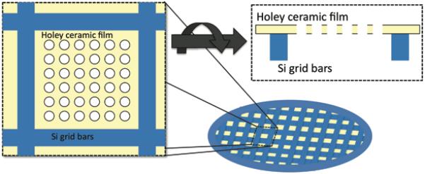
Schematic diagram of Cryomesh construction. The holey ceramic film is bonded to the Si support layer and sits above it in the side-on view. Image is adapted from material provided courtesy of Protochips Inc.

2.2 Grid Preparation and Data Collection

An additional layer of thin continuous carbon film was used in some of the datasets collected on both C-Flat and Cryomesh grids (Protochips Inc., Raleigh, NC 27606). The thin carbon on mica was a generous gift from Theresa Ruiz and Michael Radermacher of the Univ. of Vermont. The thin carbon was placed on the grids by floating the carbon off the mica onto the surface of distilled water and then picking up the carbon using the grids. The grids were then allowed to dry before use. All grids were glow discharged in a FEI Solarus plasma cleaner for 3 seconds (Ar/O₂ mix) prior to applying the specimen, which was then vitrified in liquid Ethane using a FEI Vitrobot and imaged using an Oxford CT3500 side-entry cryo-stage inserted into an FEI F20 electron microscope. All images were acquired using the software package Leginon (Suloway et al., 2005) in conjunction with its automated tilted data collection module (Yoshioka et al., 2007) to collect single-tilt images, RCT tilt pairs, and OTR tilt pairs at magnifications of 50,000X.

Three single-particle cryo datasets where collected at 45° tilt on the Cryomesh grids, one with an additional layer of thin continuous carbon. Similarly, three datasets at 45° tilt were collected on C-Flat grids with one of the datasets also containing an additional layer of thin carbon. Three large single-particle cryo datasets collected at 0° tilt were used as controls for the quantitative comparisons of BIM between grid types. The size of each of these datasets is given in Figure 5.

Figure 5.

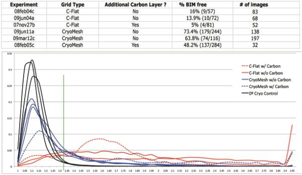
At the top is a table with datasets that were evaluated by eye and their scores. Below is a graph with histograms of the computed scores for several different datasets. In black are 0° vitreous ice datasets on C-Flats as controls. Note the very large peak in the ~1.1 range. In blue are the 45° Cryomesh datasets, and in red are the 45° C-Flat datasets. The dashed lines represent the datasets that had an additional layer of thin carbon placed on the grids. Note that while the C-Flat w/ carbon dataset has improved slightly, the majority of the improvement comes at a level where there is still noticeable BIM, ~1.6. Likewise the Cryomesh w/carbon dataset has a much smaller peak in the low score range ~1.15 compared to the unaltered Cryomesh datasets. For comparison to the manual evaluation in the Table above, the green line denotes the score that most closely corresponds to where BIM becomes visually discernible.

2.3 Evaluation of BIM in Images

Images were evaluated both by eye and by using a computational algorithm. Evaluations by eye included careful study of the images themselves, and also study of the CTF Thon rings in their power spectrums. Images that showed noticeable BIM in as little as 5% of their total area where marked as ‘bad’, but no attempt was made to measure the severity of the BIM or the size of affected areas. Toward this end, we created a novel computational assessment to quantitatively measure both the extent and severity of BIM in individual images. Historically, BIM has been most commonly evaluated in the context of 2D crystal diffraction, where its effects are easily quantified by measuring the intensity falloff of the diffraction pattern, usually in a direction perpendicular to the tilt axis. In our case, however, we were far more interested in reducing the extent of BIM in single-particle images, where the appearance of BIM is instead observed as different parts of the image appearing blurred in different directions (Figure 4).

To obtain a numerical measure of BIM from such images we attempted to determine the asymmetry in the power spectrum envelope at multiple locations within each image. Occurrence of BIM affects this envelope in several ways, most commonly by attenuating high-resolution information perpendicular to the tilt-axis, but in our case by also causing observable attenuation in the direction of the local blurring. To measure this we broke our 4096² pixel images into 1024² pixel windows with 512² pixel overlaps. For each individual window a power spectrum was calculated, then the center 100² pixels of the spectrum were extracted, Gaussian blurred (σ=3), and histogram normalized from 0.0 to 1.0 so that 1% of the pixels were clipped to the largest and smallest values. The normalized center peak of the power-spectrum was then ‘extracted’ by flood filling from the origin and only accepting pixel values > 0.3. These fully processed peaks were then summed radially, between 4-30 pixels, at 1° angular increments and the maximum ratio of these sums in perpendicular directions was used as a measure of charging. In theory, a perfect score of 1.0 would indicate that no BIM was present (since the peak would be symmetrical), although realistically, many other factors can affect this score including noise, gun tilt misalignment, objective and condenser astigmatism, strong edges in the image, etc. Care was taken to ensure that the influence of these other factors was minimized or maintained between datasets. As a result we are confident that this evaluation provided a good quantitative measurement of the relative performance between datasets. Figure 4 is a visual depiction of this process carried out on an example image from one of the 45° Cryomesh datasets. If this method were applied to a power spectrum exhibiting obvious Thon rings, then the resulting output would extract an area inside the first Thon ring, but would be guided less by the shape of this ring and more by the overall intensity falloff caused by the envelope within this area. Because of the small size of the windows being examined, Thon rings are often not visible, but the shape of this intensity falloff is a low-resolution ‘feature’ of the power spectrum that can be measured with far more confidence than the CTF could be.

2.4 Measuring Ice Thickness and Flatness

To evaluate variations in ice thickness over imaged areas we aligned the beam-shift axis with the microscope goniometer axis so that y-axis beam shifts moved along the goniometer tilt axis. Narrow channels < 180nm in width were etched through the ice in previously imaged areas by shifting a tightly focused beam across the region whilst simultaneously varying the size of the beam. In the ideal situation this resulted in bilaterally symmetrical hourglass-shaped channels that were then imaged at both 0° and 45°. Variations in the channel width allowed for easier and more accurate alignment of the channels between tilt pairs, and disruption of the bilateral symmetry provided indication of any large mechanical changes that occurred in the ice layers under subsequent exposures.

The channel tilt pairs were aligned by affine transformation of the 0° image to bring it into register with the 45° image, taking into account the foreshortening expected by the 45° tilt angle, and maximizing the alignment between features in the image (particles, edges, corners, etc.). These alignments allowed for the clear visualization of the ice thickness over imaged regions and its variations. In the case of images taken over thin carbon, alignment between the 0° and 45° proved unnecessary, as the carbon/ice and ice/vacuum interfaces both created enough contrast to make the ice layer clearly visible in the tilted image.

3. Results and Discussion

3.1 Physical Characterization of Cryomesh

Cryomesh grids have a colored sheen that is visible to the naked eye when viewed under direct lighting at the correct angle (fluorescent lighting works best). This color is due to the thin ceramic film layer (Figure 2A) and the hue is typically consistent within individual grids and is most likely related to the thickness of this layer. When viewed with this support film facing toward the viewer, the coloring is apparent over both the center of the grid and the outside silicon support ring. This side of the Cryomesh grid is equivalent to the “carbon-side” of conventional carbon-on-copper grids, as the film is above the support bars (Figure 1), and is a more appropriate surface for the application of sample or additional support films. When the same grid is flipped over and viewed from the other side, the outside support ring becomes a neutral mirror surface, while the central support area retains the same colored sheen. This can be seen in Figure 2B, where the outside support ring appears white, whereas if the same grid were flipped over, it would be colored as strongly as any of the other grids imaged in Figure 2A. Checking for this difference is the easiest way to quickly determine which side of the grid is which during sample preparation.

Figure 2.

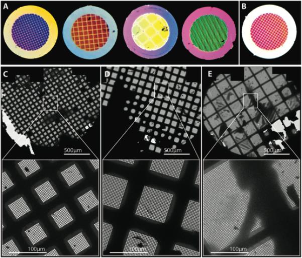
A visual characterization of Cryomesh grids. A) Cryomesh grids as imaged under standard fluorescent lighting with the ceramic silicon layer on the side of the grid facing the viewer. The colors of the grids are related to the thickness of this film layer (see Figure 1) and extend over the outside support ring since the film layer is above the support layer when viewed from this side. B) Another Cryomesh grid that has been flipped over so that the film layer is facing away from the viewer and is on the other side of the support layer. In this case, the outside support ring now has neutral, rather than colored appearance. The outside support ring of all of the grids in panel A would have a similar appearance if they were flipped over. C,D,E) low magnification (49X) and higher magnification (500x) images of different Cryomesh grids with different mesh sizes. All have samples preserved in vitreous ice. Most interesting is the grid in panel E, which has a very large mesh size, with each square containing thousands of holes and even ice distribution.

Cryomesh grids are very rigid and handle much as one would expect thin glass chips to handle - they are fragile and take some practice to manipulate adeptly. The samples received from ProtoChips Inc. came in several different configurations, with square meshes ranging from ~600 mesh (~90 um²) equivalents all the way to ~9 mesh (700 um²) (Figure 2C,D,E). We found the larger mesh sizes particularly exciting since, anecdotally, they tended toward thinner, more consistent ice thickness, and more efficient data collection (Figure 2E). These large mesh sizes are also particularly well suited for Cryomesh since conventional support films, such as carbon, could not easily span such large distances without breaking or sagging. We also tested grids with rectangular meshes of dimensions ~200um by ~50um. The diameter of the holes in the support films of all of the grids were ~2.4um and their centers were spaced ~3.9um apart. It should also be mentioned that, in principle, Cryomesh grids could be produced from any reasonably designed pattern.

To measure the thickness of the Cryomesh support film we tilted the grids to 45° in the microscope and measured the length of ridges found at the edges of holes (Figure 3A). While not exact, our measurements indicate that film thickness varied between grids, from ~750 to ~1300Å, but was relatively constant within individual grids, ±30Å. This thickness makes it difficult, but not impossible, to achieve a thin layer of vitreous ice during freezing. Measurements of specific holes showed that ice thicknesses of less than 200Å could be found in some of the Cryomesh datasets. Unfortunately, this thin ice was usually formed from liquid having a meniscus and was thus curved and likely under tension (which, as we discuss later, may affect BIM). A high-magnification (50,000X) image of the Cryomesh support film (Figure 3B) shows that the paracrystalline film creates strong fringes, similar to bend contours, which make it difficult to focus the microscope by eye. These diffraction fringes also make it difficult to focus using beamtilt induced image shift since the fringes are a major source of image contrast and shift unpredictably. The support substrate does, however, exhibit clear Thon rings when exposed sufficiently (Figure 3C), which makes it possible to focus via direct observation of the CTF in the power spectrum. Since the data acquisition software Leginon (Suloway et al., 2005) focuses using beam-tilt, we selected the edges of holes as our focus locations so that the edge contrast, rather than features in the film, would dominate the focusing process.

Figure 3.

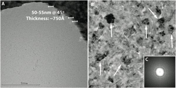
A) High magnification, 29,000X of a Cryomesh hole with vitreous ice at 45° tilt. Along the edges of the hole ridges can be seen that are left behind from the manufacturing process. By measuring the length of these ridges in projection we can estimate the thickness of the support substrate. B) An image taken over the ceramic support substrate, with examples of the features that are artifacts of the ceramic material. These would shift and disappear/reappear if the stage where tilted or the beam-tilt changed. C) The power spectrum of the image in panel B.

The electrical resistivity of the Cryomesh grid substrate at room temperature is 2-4×10⁻⁴ Ωm (thickness dependent), which supports the claim that the silicon ceramic substrate does indeed conduct electrons better than amorphous carbon (~1 Ωm @ 220Å thickness) (Rhinow and Kühlbrandt, 2008). Like carbon, whose conductivity decreases with temperature (Rhinow and Kühlbrandt, 2008), the Cryomesh support layer becomes less conductive at low temperature but at a slower rate than carbon, so that at liquid nitrogen temperatures (77°K), the Cryomesh substrate is still orders of magnitude more electrically conductive than carbon. The thermal expansion coefficient (CTE) of the Cryomesh support is 4.2×10⁻⁶ K⁻¹. Thermal expansion coefficients become important when combinations of different materials are used in cryo-preservation, since ill-matched partners can cause ‘crinkling’ deformations of the support layer upon temperature changes. This crinkling is especially detrimental in the case of 2D crystal imaging, as non-flat crystals diffract poorly (Vonck, 2000). In the case of thin carbon, it has been shown that Molybdenum grids result in far less ‘cryo-crinkling’ than copper grids (Booy and Pawley, 1993), presumably because the CTEs of molybdenum and carbon are better matched than those of carbon and copper. This is fortunate, as the CTE of Cryomesh is similar to that of Molybdenum, indicating that Cryomesh might also make a suitable substrate for additional carbon layers.

3.2 Are Cryomesh better than standard Cu grids for cryo RCT/OTR?

Compared to standard holey carbon-on-copper grids, Cryomesh grids have some advantages that are immediately apparent. The first is that they can be easier to collect data with, especially when using automated data collection software. The contrast between the film support and ice, and the regularity and flatness of the grids make computer pattern matching easier and sample z-height more consistent. Furthermore, the grids appear to be more stable in the microscope– when using our side-entry specimen holder it was not uncommon for specimen drift to end within a minute of changing stage tilt from 0° to 45°. There are, of course, many factors that affect stage stability, so this observation may not be universal.

Unfortunately these advantages only become apparent after grids with suitable ice have been inserted into the microscope. Cryomesh grids are extremely fragile and the thickness of the support substrate tends to create thicker ice than desired (a benefit is that ice tends to be more consistent across a grid). The grids are also extremely susceptible to shattering while being handled. They can break easily if squeezed too strongly with tweezers or if used in specimen stages with push-into-place style clip rings. Hence, the use of reverse-tweezers and stages with screw-on or c-clip style clip rings is advised. We also augmented our standard cryo loading procedure by ‘washing’ the end of the stage with liquid nitrogen before insertion into the microscope to prevent the entry of stray shards into the column.

To evaluate the performance of Cryomesh grids with regards to BIM, we collected large datasets of Cryomesh and C-Flat grids at 45° tilt. Datasets of C-Flat grids at 0° were used as negative controls as these datasets contain virtually no (visible) BIM. The first empirical observation we made was that BIM seemed lessened in the 45° Cryomesh datasets when compared to the 45° C-Flat datasets, and that when present, was far more likely to be localized to sub-regions within images (Figure 4). A careful visual assessment (see Methods 2.3) of the datasets led us to estimate that 64-74% of the tilted Cryomesh images did not show any noticeable indication of BIM compared to 14-16% for the C-Flat grids. Unfortunately this assessment did not take into account the locality or severity of BIM within individual images. Many of the images exhibiting BIM in the 45° Cryomesh datasets contained large areas from which useable data could still be extracted whereas, “bad” images from the 45° C-Flat datasets were more uniformly distorted and less salvageable. It was, however, too difficult to measure this aspect of improvement by visual inspection, so we developed an algorithm to quantitatively make the comparison.

For the computer assessment, individual images were sub-divided into smaller images that were each scored individually for the presence of BIM (see Methods 2.3). Scores of 1.0 where ideal, indicating regions in which BIM was causing no local blurring, while higher scores indicated regions of increased distortion. In Figure 5 histograms of these scores for each of the datasets are plotted. The 0° cryo datasets used as controls showed large peaks in the low scoring range (<1.2), indicating that a very large percentage of the dataset had little to no measureable BIM. As expected, the C-Flat grids at 45° performed worst, with larger and more evenly distributed scores than the other datasets, an indication that BIM was both more frequent and more severe. Conversely, the Cryomesh grids at 45° did far better than the C-Flat grids at 45°. Most noticeably, the 45° Cryomesh datasets showed strong peaks in the <1.2 range similar to those of the 0° controls, while the 45° C-Flat datasets did not. This indicates that a large percentage of the 45° Cryomesh dataset scored as well by this measure as the (essentially) BIM-free controls. It should also be mentioned that the control datasets used in this comparison resulted in reconstructions of GroEL (Stagg et al., 2008) and P22 tail machinery (Lander et al., 2009) at sub-nanometer resolution, which indicates, all other things being equal, that a large percentage of the tilted Cryomesh datasets might be of similar quality.

Although the computer scoring provided a more nuanced evaluation of grid performance, it was a novel method, and as such, we found it important to verify the results by manual evaluation. Overall we found that the scoring of images was consistent and appropriate, i.e. regions of visibly similar BIM scored similarly across datasets, and higher scores corresponded very well with perceived increases in BIM. We also found that it was, in general, difficult to discern BIM in areas with scores less than ~1.35, though we have no reason to doubt that lower scores still reflect a slight, though unnoticeable, amount of image degradation. Nevertheless, if a score of 1.35 is used as a hard cutoff so that the computer scoring can be compared to the manual scoring, then 98-99% of the control images do not show noticeable BIM versus 74-80% for Cryomesh and 13-18% for C-Flats. This analysis reinforces our earlier observation that Cryomesh grids improve the results of imaging at tilt. Furthermore, the higher percentage given by the computer assessment compared to the visual assessment is likely due to the BIM on the Cryomesh grids being a more localized phenomenon.

In an attempt to further improve our performance at 45°, we reasoned that the addition of a second layer of thin continuous carbon (TCC) over the Cryomesh and C-Flat grids would help reduce BIM by adding an additional conductive layer that would span the holes in the support film. Unexpectedly, the result of this additional layer was that the rate of BIM actually increased rather than decreased for the Cryomesh grids. This can be seen in Figure 5, where the nice peak at <1.2 seen for the unmodified Cryomesh grids becomes flatter and skewed toward higher scores in the TCC Cryomesh dataset. Conversely, the additional carbon layer resulted in a slight improvement for the C-Flat grids, but this improvement seemed to only reduce the overall severity of BIM rather than eliminate it. This can be seen in Figure 5 as a peak that forms in the score range 1.35 - 1.75 where BIM is more moderate, but still noticeable. So while it appears that there is some benefit to an additional carbon layer, the benefit is marginal and/or unpredictable. One possible reason why the additional carbon layer was not as effective as hoped is that carbon is known to be a poor conductor at liquid nitrogen temperatures, limiting its potential assistance in this area. These results also suggested an alternative explanation for the improvement seen in the Cryomesh datasets. It appeared that the small benefit provided by additional carbon film was already subsumed by similar benefits already provided in the Cryomesh substrate, so we began to ponder how an additional carbon layer might increase occurrence of BIM. We explore this second possibility next.

3.3 What are the reasons for the Cryomesh improvements?

Despite their greatly increased conductivity and rigidity, the Cryomesh grids were not entirely free of BIM, as some 20-30% of the images still exhibited the effect. This indicates that conductivity and rigidity may not be the sole factors involved in the occurrence of BIM, or that their involvement is somewhat indirect. This hypothesis was further fleshed out when we observed that additional layers of thin carbon film increased the frequency of BIM rather than decreased it– the opposite of what we had expected.

One possible explanation for this observation was that the ice on the thin-carbon coated (TCC) Cryomesh grids often showed clear indications of thickness variations while the ice on the standard Cryomesh grids often did not. Another common observation was that occurrences of BIM on a standard Cryomesh grid were often clustered within specific regions of the grid, and that these regions were more likely to contain variations in ice thickness or contamination. Based on statistics from the collected datasets, an image taken on a Cryomesh grid was 23X more likely to contain BIM if any image taken at an adjacent hole had also exhibited BIM. This led us to believe that the geometry of the sample/ice itself (thickness, curvature, fractures, etc.) might be playing a strong, though not necessarily unique, role in whether BIM was observed or not, and that variations in this geometry over large areas, i.e. several holes or even an entire grid square, was important. Based on this hypothesis, it is easy to see how a flat, rigid surface, such as Cryomesh, might greatly improve the odds of favorable imaging conditions but not guarantee them.

In an attempt to verify the importance of ice geometry, we noted variations in ice thickness over the holes on C-Flat and Cryomesh grids, and related these observations back to occurrences of BIM. To achieve a more direct visualization of ice thickness we imaged channels that we had cut through previously imaged areas (see Methods 2.4), 18 for the C-Flat and 28 for the Cryomesh. Figure 6 shows several examples of these channels for comparison. The first observation we made was that non-uniform ice was more likely to be associated with BIM, since 81% (22 of 27) of such channels showed it. Of these, 89% (16 of 18) of the channels that had obvious curvature in the ice, and 66% (6 of 9) that had a simple gradient, showed BIM. It also appeared that the magnitude of the ice variations seen in the channels of the C-Flat grids were greater than that of the Cryomesh grids. Finally, the rate of BIM in images whose channels did not show any obvious ice variations were 30% (3 of 10) for Cryomesh and 43% (3 of 7) for C-Flats.

Figure 6.

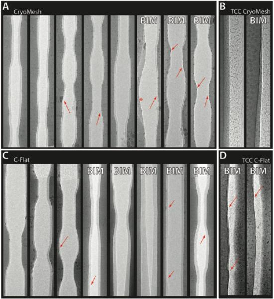
A gallery of channels that have been cut through the ice layers on different grid types. For the images in panels A and C, 45° and 0° images of the same area were aligned so that the thickness and variations in the ice layer could be easily observed. Further details can be found in Methods 2.4. A) Cryomesh grids B) carbon-coated Cryomesh C) C-Flat and D) carbon-coated C-Flat. Areas with subtle thinning or curvatures in the ice are denoted with red arrows. The red asterisk marks locations where the bilateral symmetry has been broken, likely due to ice movement. Channels that belong to images that exhibited BIM are marked by an upper-case ‘BIM’. Note that overall, the Cryomesh ice is more regular in flatness and thickness than the C-Flat ice. Also note that additional carbon film makes ice more irregular in thickness, and even more in flatness. The thin carbon coating also allows one to visualize the channel thickness without having to align the 0° images with the 45° images (though we did this anyways to confirm what we saw). Presumably this is because the ice/carbon interface creates contrast in addition to the ice/vacuum interface.

These results possibly indicate that the geometry of the sample (in our case the vitreous ice) has a role in BIM that can be as important as the conductivity of the support substrate. Unfortunately this analysis was very time consuming and needs to be investigated in more depth and far greater numbers to draw more quantitative results. Nonetheless, it showed that overall, the Cryomesh ice was flatter than the C-Flat ice, and that there was some correlation between the quality of this ice and the BIM observed.

3.4 Conclusions

Cryomesh grids led to a marked improvement in the acquisition of high-quality images of tilted ice-embedded specimens. This was verified both by visual examination, and by implementing an algorithm to computationally evaluate images. Among the conclusions we drew from this comparison were:

1. Cryomesh grids can be successfully used to embed specimens in vitreous ice and image them in the microscope.

2. It is possible to quantitatively assess and compare the effect of BIM on single-particle images

3. Cryomesh grids reduce the frequency and severity of BIM, and also increase its localization when compared to holey carbon-on-copper grids.

Despite their superiority, however, these grids did not abolish the appearance of BIM. Likewise, it was not entirely clear whether the increased conductivity of these grids resulted in the observed improvements, or if the increased rigidity and flatness also played a role by reducing mechanical flexibility and/or helping to create more favorable ice conditions. Our attempts to link ice conditions to occurrences of BIM provide an early indication of such a correlation, but this conclusion is still preliminary. In any case, Cryomesh presents a pragmatic, multi-faceted approach to helping solve the problem of BIM, regardless of the underlying mechanism. As a new technology, we also expect that many improvements to their design such as ease of handling, improved performance, etc., are still in the future.

References

- Booy FP, Pawley JB. Cryo-crinkling: what happens to carbon films on copper grids at low temperature. Ultramicroscopy. 1993;48:273–280. doi: 10.1016/0304-3991(93)90101-3. [DOI] [PubMed] [Google Scholar]
- Bottcher B. Electron cryo-microscopy of graphite in amorphous ice. Ultramicroscopy. 1995;58:417–424. [Google Scholar]
- Brink J, Sherman MB, Berriman J, Chiu W. Evaluation of charging on macromolecules in electron cryomicroscopy. Ultramicroscopy. 1998;72:41–52. doi: 10.1016/s0304-3991(97)00126-5. [DOI] [PubMed] [Google Scholar]
- Chen JZ, Sachse C, Xu C, Mielke T, Spahn CM, Grigorieff N. A dose-rate effect in single-particle electron microscopy. Journal of structural biology. 2008;161:92–100. doi: 10.1016/j.jsb.2007.09.017. [DOI] [PMC free article] [PubMed] [Google Scholar]
- Downing K, Sui H, Auer M. Electron Tomography: A 3D View of the Subcellular World. Analytical Chemistry. 2007;79:7949–7957. doi: 10.1021/ac071982u. [DOI] [PubMed] [Google Scholar]
- Dubochet J, Lepault J. Cryo-electron microscopy of vitrified water. Journal de Physique Colloques. 1984;45:84–94. [Google Scholar]
- Glaeser RM. Electron crystallography of biological macromolecules. Annual Review of Physical Chemistry. 1985;36:243–275. [Google Scholar]
- Glaeser RM. Retrospective: Radiation damage and its associated Information Limitations. Journal of structural biology. 2008;163:271–276. doi: 10.1016/j.jsb.2008.06.001. [DOI] [PubMed] [Google Scholar]
- Glaeser RM, Downing K. Specimen Charging on Thin Films with One Conducting Layer: Discussion of Physical Principles. Microscopy and Microanalysis. 2004;10:790–796. doi: 10.1017/s1431927604040668. [DOI] [PubMed] [Google Scholar]
- Gyobu N, Tani K, Hiroaki Y, Kamegawa A, Mitsuoka K, Fujiyoshi Y. Improved specimen preparation for cryo-electron microscopy using a symmetric carbon sandwich technique. Journal of structural biology. 2004;146:325–33. doi: 10.1016/j.jsb.2004.01.012. [DOI] [PubMed] [Google Scholar]
- Henderson R. Image contrast in high-resolution electron microscopy of biological macromolecules: TMV in ice. Ultramicroscopy. 1992;46:1–18. doi: 10.1016/0304-3991(92)90003-3. [DOI] [PubMed] [Google Scholar]
- Henderson R, Glaeser RM. Quantitative analysis of image contrast in electron micrographs of beam-sensitive crystals. Ultramicroscopy. 1985;16:139–150. [Google Scholar]
- Lander GC, Khayat R, Li R, Prevelige PE, Potter CS, Carragher B, Johnson JE. The P22 tail machine at subnanometer resolution reveals the architecture of an infection conduit. Structure. 2009;17:789–99. doi: 10.1016/j.str.2009.04.006. [DOI] [PMC free article] [PubMed] [Google Scholar]
- Leschziner AE, Nogales E. The orthogonal tilt reconstruction method: an approach to generating single-class volumes with no missing cone for ab initio reconstruction of asymmetric particles. Journal of structural biology. 2006;153:284–99. doi: 10.1016/j.jsb.2005.10.012. [DOI] [PubMed] [Google Scholar]
- Radermacher M. Three-dimensional reconstruction of single particles from random and nonrandom tilt series. Journal of electron microscopy technique. 1988;9:359–94. doi: 10.1002/jemt.1060090405. [DOI] [PubMed] [Google Scholar]
- Rhinow D, Kühlbrandt W. Electron cryo-microscopy of biological specimens on conductive titanium-silicon metal glass films. Ultramicroscopy. 2008;108:698–705. doi: 10.1016/j.ultramic.2007.11.005. [DOI] [PubMed] [Google Scholar]
- Stagg SM, Lander GC, Quispe J, Voss NR, Cheng A, Bradlow H, Bradlow S, Carragher B, Potter CS. A test-bed for optimizing high-resolution single particle reconstructions. J Struct Biol. 2008;163:29–39. doi: 10.1016/j.jsb.2008.04.005. [DOI] [PMC free article] [PubMed] [Google Scholar]
- Suloway C, Pulokas J, Fellmann D, Cheng A, Guerra F, Quispe J, Stagg S, Potter CS, Carragher B. Automated molecular microscopy: the new Leginon system. Journal of structural biology. 2005;151:41–60. doi: 10.1016/j.jsb.2005.03.010. [DOI] [PubMed] [Google Scholar]
- Vonck J. Parameters affecting specimen flatness of two-dimensional crystals for electron crystallography. Ultramicroscopy. 2000;85:123–129. doi: 10.1016/s0304-3991(00)00052-8. [DOI] [PubMed] [Google Scholar]
- Yoshioka C, Pulokas J, Fellmann D, Potter CS, Milligan RA, Carragher B. Automation of random conical tilt and orthogonal tilt data collection using feature-based correlation. Journal of structural biology. 2007;159:335–46. doi: 10.1016/j.jsb.2007.03.005. [DOI] [PMC free article] [PubMed] [Google Scholar]