Fitness flux and ubiquity of adaptive evolution

Abstract

Natural selection favors fitter variants in a population, but actual evolutionary processes may decrease fitness by mutations and genetic drift. How is the stochastic evolution of molecular biological systems shaped by natural selection? Here, we derive a theorem on the fitness flux in a population, defined as the selective effect of its genotype frequency changes. The fitness-flux theorem generalizes Fisher’s fundamental theorem of natural selection to evolutionary processes including mutations, genetic drift, and time-dependent selection. It shows that a generic state of populations is adaptive evolution: there is a positive fitness flux resulting from a surplus of beneficial over deleterious changes. In particular, stationary nonequilibrium evolution processes are predicted to be adaptive. Under specific nonstationary conditions, notably during a decrease in population size, the average fitness flux can become negative. We show that these predictions are in accordance with experiments in bacteria and bacteriophages and with genomic data in Drosophila. Our analysis establishes fitness flux as a universal measure of adaptation in molecular evolution.

Adaptive processes have taken center stage in molecular evolutionary biology. Deep sequencing of populations opens unprecedented opportunities to trace the genomic basis of adaptation in population-genetic studies within and across species as well as in time series of evolution experiments. Various methods are used to infer natural selection from such data; however, their results lack a common gauge and are sometimes difficult to compare. This paper develops the concept of fitness flux in a population as a generic measure of adaptation applicable to molecular data. Whereas fitness characterizes the state of a population at a given point in time, fitness flux can be accumulated in a population’s history over a period (a precise definition of this quantity will be given below). Fitness flux, not fitness, turns out to be the right variable to show that adaptive evolution is a generic state of natural populations. The notion of fitness flux is already implicitly contained in Fisher’s fundamental theorem of natural selection (1), which states that any fitness difference within a population leads to adaptation in an evolution process governed by natural selection alone. The fitness flux of this deterministic process equals the (additive) fitness variance in the population. Hence, the flux is positive when adaptation occurs and zero otherwise.

Generalizing this picture to realistic processes of molecular evolution has been a long-standing problem (2–8). The solution presented here involves a number of important conceptual steps. First, molecular processes are always stochastic because of genetic drift and mutations, and we include these forces into a stochastic theory of fitness flux. Second, we extend the observation of this dynamics to the time scales of genomic data, describing populations by histories of genotype composition and demography that may extend beyond their coalescence time. Third, natural selection itself is treated as dynamic on these time scales. We generalize static fitness landscapes, a concept introduced by S. Wright (9), to explicitly time-dependent models of selection referred to as fitness seascapes. The time dependence of selection reflects the changing ecology of a species. It has complex and opposing effects on adaptation (10–15): rapid fluctuations enhance the stochasticity of the evolutionary process and impede long-term adaptation (11), but persisting changes open windows of positive selection and are the very cause of adaptive evolution and fitness flux (13, 15). The production of fitness flux by adaptive processes is a nonequilibrium phenomenon and does not necessarily imply any increase in fitness. Surprisingly, this production obeys a general theorem, which provides a basis for quantifying adaptation in stochastic evolution. The theorem and its proof establish an important conceptual link between evolutionary genetics and stochastic nonequilibrium thermodynamics. A close analogy of the fitness-flux theorem to its deterministic counterpart, Fisher’s theorem, emerges in the case of stationary evolution. The average fitness flux is positive in nonequilibrium stationary states , which are associated with adaptive evolution (15). The flux is zero at evolutionary equilibrium, where no adaptations occurs. The power of the fitness-flux theorem will be shown by a number of applications to evolution experiments in microbes and to cross-species genome comparison in flies.

Theory of Fitness Flux

Population Histories and Fitness Flux.

We start by introducing the notion of fitness flux and its relationship to fitness. Consider first the microevolution of a population containing a resident and a mutant genotype. The genotype evolution of the population can be described by a series of observations x = (x₀, x₁, …, x_n) of mutant frequencies at successive times (t₀, t₁, …, t_n), which we refer to as the history of the population. Natural selection governs this process by a difference in reproductive rate of the mutant against the resident genotype, s, which may depend on frequencies and time. Here, we consider selection coefficients s(x, t) with persistence times of many generations that affect the evolution of genotype frequencies and can be measured, for example, by growth-competition experiments in a microbial population. Measurements of population histories are assumed to be sufficiently dense so that the changes in selection as well as frequency changes (Δx_i = x_i+1 − x_i) in each time interval (Δt_i = t_i+1 – t_i) are small. The fitness flux can then be defined as a measure of adaptation at a given point of the population history: φ(t_i) = s(x_i, t_i)Δx_i/Δt_i is the product of the selection coefficient and the rate of frequency change. The cumulative fitness flux (Eq. 1)

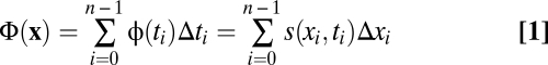measures the total adaptation of the entire population history (13). For a history containing a substitution process (i.e., a transition from initial frequency x₀ = 0 to final frequency x_n = 1) under constant selection, the flux Φ equals the selection coefficient s of the new genotype against the old genotype. This picture is easily extended to sequences of length L with 4^L possible genotypes, where x and s become vectors with 4^L – 1 independent components. The genotype-based approach is useful for compact genomic units such as transcription factor-binding sites, where recombination can be neglected. Our results equally apply to the evolution of populations measured by allele frequencies at individual genomic loci (i.e., by vectors x and s with 3L independent components). This picture, which neglects correlations between coexisting alleles at different genomic loci (linkage disequilibrium), is valid in populations with sufficiently efficient recombination (SI Text). Including all accessible sequence states in the description of population histories, not just those coexisting at a given point in time, makes it possible to describe processes over longer evolutionary time. Such processes involve fixed population states interspersed with polymorphic time intervals and may contain substitutions at multiple genomic loci, which contribute additively to the cumulative fitness flux.

Fitness Land- and Seascapes.

A particularly intuitive picture of fitness flux emerges if the selection coefficients are the gradient of a time-independent fitness landscape. The relation s(x) = ∇F(x) defines this landscape up to an arbitrary constant (and implies that F differs in general from the mean population fitness; SI Text). Selection coefficients at one locus depending on the allelic state at another locus define fitness interactions between genomic loci (epistasis); fitness landscapes with pervasive epistasis are often called rugged. Such interactions generate linkage disequilibrium within a population and also correlations between alleles fixed at different genomic loci in subsequent states of a population history, which reflect compensatory modes or complex adaptive pathways of molecular evolution (16). In any fitness landscape, the frequency change Δx_i in each time interval between successive measurements results in a fitness change Δx_i∇F(x_i), as illustrated in Fig. 1A. By Eq. 1, the cumulative fitness flux of the entire population history is then simply the fitness change between the initial and final population, Φ(x) = F(x_n) – F(x₀). This picture can be extended to evolution in a fitness seascape F(x, t) describing time-dependent selection coefficients s(x, t) = ∇F(x, t), as illustrated in Fig. 1B. The fitness flux (Eq. 1) takes the form and remains a well-defined observable of the adaptive process, because it involves only growth-rate differences between genotypes within a population at a given point in time. However, the fitness flux is no longer equal to the fitness difference between the initial and final population. This is because its definition does not include the explicit fitness change during a population history, , which depends on arbitrary constants and is unrelated to the adaptive process. In the example of Fig. 1B, the initial state is fitter than the final state in the original landscape, F(x₀, t₀) > F(x_n, t₀), but the roles of both states are reversed in the final landscape, F(x_n, t_n) > F(x₀, t_n). The example shows that fitness differences between populations at different times cannot even be defined in an unambiguous way under time-dependent selection and hence, cannot serve as a universal measure of adaptation. The same is true in more general cases in which the selection coefficients s(x, t) cannot be expressed as gradient of any fitness function F(x, t). An example is cyclic selective advantage between three or more genotypes as in the well-known rock-paper-scissors game, which is shown in Fig. 1C and has been observed, for example, in bacterial and lizard populations (22, 23). We include these cases into the picture of fitness seascapes, associating nongradient selection coefficients s(x, t) with water currents unrelated to the height pattern F(x, t) of the waves. Fitness flux φ and cumulative flux Φ as given by Eq. 1 are well-defined measures of response to selection pressures for population histories in any fitness seascape. This is why we can infer fitness fluxes, but not fitness differences, between populations from experimental and genomic data. Positive values of φ, or an increase of Φ, signal adaptation in a population history. But when does Φ increase?

Fig. 1.

Evolution in fitness landscapes and seascapes. The evolutionary history of a population is described by a series of genotype or allele frequency states x = (x₀, …, x_n) at times (t₀, …, t_n) (here, n = 3). Evolutionary time increases between the initial state (◇) and the final state (□). The cumulative fitness flux in each time interval (gray-filled vertical arrows) is the product of the frequency change Δx_i = x_i+1 – x_i between successive states (horizontal arrows) and the selection coefficient s(x_i, t_i) of this change; the cumulative flux Φ(x) of the entire history is the sum of these terms. The reverse history x^T = (x_n, …, x₀) evolves through the same states in reverse order from the initial state (□) to the final state (◇). Each transition has the opposite fitness effect as the corresponding transition of the original history, resulting in a cumulative fitness flux Φ(x^T) = – Φ(x) (the direction of all arrows is reversed). (A) Evolution in a fitness landscape F(x). The gradient of this function defines time-independent selection coefficients s(x) = ∇F(x). A linear landscape corresponds to a frequency-independent selection, and a nonlinear landscape as shown here corresponds to frequency-dependent selection. The cumulative fitness flux Φ(x) of a population history measures the fitness difference ΔF = F(x_n) – F(x₀) between initial and final population. In general, the function F(x) is not equal to the mean population fitness, as discussed in SI Text. (B) Evolution in a fitness seascape F(x, t). The gradient of this function defines time-dependent selection coefficients s(x, t) = ∇F(x, t). The cumulative fitness flux of a population history is defined in terms of selection coefficients and frequency changes as before. However, it no longer equals the fitness difference between initial and final population, because its definition does not include the explicit time dependence of fitness during the history that is unrelated to adaptation (unfilled vertical arrows). (C) Evolution in a fitness seascape with selection coefficients s(x, t) not of gradient form. The example shows cyclic selective advantage as in the rock-paper-scissors game (i.e., each of the transitions from x₀ to x₁, from x₁ to x₂, etc., and from x₂ to x_n = x₀ involves a positive selection coefficient). The fitness flux is defined as before and is again unrelated to a fitness difference between final and initial population state.

Deterministic Versus Stochastic Evolution, Fisher’s Theorem.

The first to address the increase of Φ and to establish a measure of adaptation different from fitness was R.A. Fisher in his fundamental theorem (1), whose rationale has been elucidated decades later by Price (25) and Ewens (26). Fisher’s partial rate of fitness increase caused by natural selection (25) is just the fitness flux φ defined for allele frequencies at genomic loci (SI Text). The fundamental theorem equates this flux to the additive genetic fitness variance in the population. As long as there are any fitness differences between coexisting alleles, this flux is positive (i.e., the cumulative flux Φ increases), and there is adaptation: Fisher’s populations move uphill on fitness landscapes. However, the theorem is valid only under the restrictive assumption that evolution is deterministic and dominated by natural selection, which excludes mutations and genetic drift. Hence, Fisher’s theorem applies only to microevolution of established alleles in the limit of large populations under strong selection, a regime that is violated by low-frequency alleles in any finite population.

To describe realistic processes of molecular evolution over longer evolutionary times, we must include mutations and genetic drift in our scenario. These stochastic evolutionary forces compete with natural selection and invalidate Fisher’s theorem. The fixation of slightly deleterious mutations and mutation load are well-known examples for such effects. Thus, the fitness flux of an individual population can become negative: stochastically evolving populations can move downhill on fitness landscapes (27). Of course, stochastic evolutionary theory no longer addresses single populations but ensembles of evolving populations with time-dependent distributions P(x, t) of genotype or allele frequencies. The interpretation of such distributions is strictly probabilistic, because genotype space and allele-frequency space for multiple genomic loci are very high dimensional and can never be sampled by the time course of a single population or by an actual ensemble of populations. Simple observables in populations and their histories, however, can be sampled and compared with predictions of the probabilistic theory. This is the case for the theorem to be established below, which is an identity involving the cumulative fitness flux.

Evolutionary Equilibria and Fitness.

We first show how fitness and fitness flux can be evaluated in stochastic population ensembles. The evolution of the frequency distribution P(x, t) is determined by the conditional probabilities G(x′, t′, x, t) of the transition from initial frequencies x at time t to frequencies x′ at a later time t′. We define evolutionary equilibrium as a stationary (time-independent) distribution P_eq(x), which satisfies the so-called detailed balance condition G(x′, t′, x, t)P_eq(x) = G(x, t′, x′, t)P_eq(x′) for arbitrary times and frequencies. Detailed balance says that in equilibrium, the probability of any evolutionary transition equals the probability of the reverse transition. This definition is well-known in statistical physics, but it is more restrictive than the definitions in much of the population-genetics literature, where any stationary state is called equilibrium. For simplicity, we assume that the mutation-drift process in the absence of selection has an (approximate) equilibrium P₀(x). This is the case if the mutation rates are independent of time and satisfy mild additional conditions (Methods). We do not require that the actual process has reached this equilibrium. Given a neutral equilibrium, the full process in an arbitrary time-independent fitness landscape F(x) also has an equilibrium, and its frequency distribution is of remarkably simple form (Eq. 2),

(Methods). Here, N is the effective population size, and the additive constant of the fitness landscape is given by normalization of the distribution P_eq. Kimura’s (27) U-shaped distributions for a single two-allele locus at neutrality and under directional selection are classic examples of evolutionary equilibria and the fitness relation (Eq. 2). Various forms of this relation have been used to infer scaled fitness landscapes NF(x) from histograms of the distributions P₀(x) and P_eq(x) obtained from genomic data (28, 29) (for a recent review, see ref. 15). The fitness relation has an obvious information-theoretic interpretation (30): the function NF(x) is the relative log-likelihood of the distributions P_eq(x) and P₀(x), and its expectation value equals the relative (Kullback–Leibler) entropy of these distributions, N〈F〉 = H(P_eq|P₀).

Reverse Histories and Fitness Flux.

Equilibrium may be the exception rather than the rule in the evolution of biological systems under natural selection. A generic process evolves from arbitrary initial conditions in an arbitrary (time-dependent or nongradient) fitness seascape, generating a frequency distribution P(x, t) that may be far from equilibrium. This distribution can still be compared with the neutral equilibrium distribution P₀(x) by the relative log likelihood , which, however, no longer equals the scaled fitness NF(x) as in equilibrium. We now derive a nonequilibrium identity similar to Eq. 2 for the probability distribution of population histories in a given time interval (t₀, t_n). We define for each history x a reverse history x^T = (x₀^T, …, x_n^T). Starting from the point x₀^T = x_n at time t₀, the history x^T evolves through the population states of x in reverse order, and each transition has the opposite fitness effect as the corresponding transition in the original history (Fig. 1). Using methods originally developed in nonequilibrium thermodynamics (31–34), we can show that the probability of the reverse history is given by (Eq. 3)

where Φ(x) is the cumulative fitness flux and is the difference in relative log likelihood between the initial and final point of the original (forward) history (Methods).

Fitness-Flux Theorem.

We can now state the theorem: an evolutionary process with mutations, genetic drift, and selection given by an arbitrary fitness seascape satisfies the identity (Eq. 4)

The angular brackets denote an average over the probability distribution of population histories, , in a given time interval (t₀, t). Using Eq. 3, we recognize this history average as the sum , which equals unity by normalization of the probability distribution of reverse histories. The identity (Eq. 4) is a genuine nonequilibrium relation: it is valid for arbitrary initial conditions P(x, t₀) and arbitrary time-dependent selections. It belongs to a set of relations known as fluctuation theorems, which have played an important role in the nonequilibrium statistical physics of mesoscopic systems over the past decade (31–34). As an immediate consequence of Eq. 4, the fitness flux in any fitness seascape has a lower bound,

where is the relative entropy difference between initial and final frequency distribution. If the underlying assumption of existence of a neutral equilibrium is dropped, relations analogous to Eq. 4 and the inequality 5 still hold for the total nonequilibrium flux, which is the sum of fitness flux and neutral mutation flux (SI Text).

Applications of the Theorem

Population histories and fitness fluxes are increasingly accessible to experimental observation (17– 21). As an example, consider a recent experiment describing the adaptation of a bacterial population to antibiotic stress (17). This process involves five amino acid substitutions in a specific protein (i.e., 2⁵ = 32 different genotypes and 5! = 120 different population histories differing in the order of these substitutions). The selection coefficient of each substitution in each genetic background has been measured, and the cumulative fitness flux of a population history is simply the sum of the selection coefficients of its substitutions in their specified order. More generally, polymorphism and substitution data from a growing number of sequenced genomes can be used to estimate rate and selection coefficients of sequence changes (an example is discussed below). Such estimates provide copious data on fitness fluxes and adaptation on macroevolutionary scales. It can be shown, for example, that the well-known McDonald–Kreitman method (24) is a test not merely for positive selection but also for the positivity of fitness flux (13).

The fitness-flux theorem provides a classification of these observations into different scenarios of Darwinian evolution at the molecular level. We now discuss such scenarios and their relevance to experiments and genomic studies.

Evolutionary Equilibrium.

The equilibrium distribution (Eq. 2) is the unique population ensemble in which the identity holds for each population history. Numerical simulations of equilibrium populations shown in Fig. 2A illustrate the identical statistics of NΦ and for individual histories and the resulting ensemble distributions. By Eq. 3, the identity implies that the probability of any history equals that of its reverse history, , which expresses detailed balance of the equilibrium ensemble: beneficial substitutions of selection coefficient s > 0 occur at the same rate as deleterious substitutions of selection coefficient −s. Hence, the average fitness flux 〈φ〉 vanishes, and the average fitness 〈F〉 remains constant. Evolutionary equilibrium has been realized, for example, in an experiment with bacteriophages (35). Under stationary experimental conditions, the phage populations have been found to relax to constant fitness values that are independent of the previous history of the population and increase with population size, consistent with the behavior of the ensemble average 〈F〉 predicted by Eq. 2. This self-averaging of individual populations suggests that the phage genome has a sufficient number of independently evolving loci.

Fig. 2.

Fitness evolution of genomic population histories under three different scenarios of selection and demography. (A) Evolutionary equilibrium in a time-independent fitness landscape. (Upper Left) Fitness evolution of a single two-allele genomic locus (schematic). The two alleles a, b have time-independent fitness values f_a, f_b (black lines). The mean population fitness of this locus (red line) evolves by a series of beneficial or deleterious substitutions (red arrows), which have selection coefficients s = f_b – f_a and – s, respectively. This process obeys detailed balance (i.e., beneficial substitutions occur at the same rate as deleterious ones). (Lower Left) Fitness evolution of sequences with L = 12 independent two-allele loci, additive fitness and a uniform mutation rate of μ per locus. Fitness flux NΦ (red lines) and the negative of the log-likelihood change, (green lines), between initial and final population state in the interval (0, t) are shown as time series of an individual history (solid lines) and as ensemble averages over 10⁵ independently evolving populations (dashed lines). Each population history obeys the detailed balance relation (in the equilibrium ensemble, log likelihood equals scaled fitness NF). Evolutionary time is measured in units of the inverse neutral genomic mutation rate 1/μL. Polymorphism lifetimes are short, and substitution processes (vertical line segments and arrows) appear instantaneous on this time scale. For simulation details, see SI Text. (Lower Right) Histograms of NΦ (red), (green), and (blue) at a given time t = 28.8/μL for an ensemble of 10⁵ populations, with averages marked by dashed vertical lines. (B) Nonequilibrium stationary state in a stochastic fitness seascape. Diagrams are the same as in A. Selection coefficients s(t) = f_b(t) – f_a(t) at individual genomic loci fluctuate between two values following a Poisson process, which generates independent selection histories at each locus (for details, see SI Text). Because the rate of selection fluctuations is much smaller than the inverse polymorphism lifetime, a switch of selection generates a persistent window of positive selection. The average cumulative fitness flux N〈Φ〉 increases with time at a constant positive rate, signaling adaptive substitutions. Most individual population histories have a flux NΦ close to this average, but there are rare drift-dominated histories with . (C) Transitions between equilibria under demographic changes. Diagrams are the same as in A. Population size first decreases from an initial value N₀ to a bottleneck value N_b = N₀/2, remains constant during the bottleneck, and later increases to the original value N₀. This process results in time-dependent scaled-allele fitness values N(t)f_a, N(t)f_b and selection coefficients N(t)(f_b – f_a). The population decline generates a loss in scaled fitness, Δ₁H = Δ₁〈NF〉 < 0 and a negative scaled fitness flux N₀〈Φ₁〉 < 0 in the time interval (0, t₁ = 26.6/μL). The recovery in the time interval (t₁, t₂ = 57.6/μL) restores the initial fitness, Δ₂H = Δ₂〈NF〉 = – Δ₁H > 0, and generates a positive scaled fitness flux N₀〈Φ₂〉 that exceeds the flux N₀〈Φ₁〉 of the decline in magnitude (for details, see Methods and SI Text).

For the approach to equilibrium, the inequality 5 implies that the free fitness N〈F〉 – H always increases monotonically with time and is maximal at equilibrium (4, 36), which is an evolutionary analog of Boltzmann’s H theorem. Consistent with this scenario, the recent analysis of a long-term experiment of bacterial evolution under constant conditions has found an increase of fitness and a decrease of fitness flux φ over time (21).

Nonequilibrium Stationary States.

In a generic population ensemble, the maximum principles of equilibrium (4, 36) and the detailed balance condition for individual histories are violated. For any stationary nonequilibrium ensemble, the inequality 5 with ΔH = 0 predicts that the average fitness flux 〈φ〉 = d〈Φ〉/dt is a positive constant: populations steadily accumulate a surplus of beneficial over deleterious changes. Thus, adaptation takes place, although the average fitness 〈F〉 remains constant. For most individual populations, the cumulative flux over a sufficiently long time interval Δt is close to the ensemble average, Φ ≈ 〈Φ〉 = 〈φ〉Δt > 0. The full theorem (Eq. 4) shows that selection is overcome by genetic drift and in an exponentially small subset of populations. Muller’s ratchet, the scenario of degradation by an excess of deleterious substitutions, is, thus, very unlikely as a stationary process but requires, for example, a dwindling population size.

Stationary nonequilibrium evolution can be caused by time-dependent selection (15). Here, we consider a minimal stochastic fitness seascape defining independently fluctuating selection coefficients at individual genomic loci. This process generates an ensemble of populations with joint histories of selection and genotype, which is shown in the numerical simulations of Fig. 2B. In accordance with the fitness-flux theorem, the cumulative flux 〈Φ〉 in the stationary state increases at a constant positive rate 〈φ〉. Typical populations adapt to changing selection pressures by a surplus of beneficial over deleterious substitutions. Recent population-genetic studies of Drosophila genomes have shown evidence for adaptive evolution at a genome-wide level (37, 13, 38). Positive fitness flux (with values NΦ of order 10 per genomic substitution) (13) has been inferred from joint estimates of rate and average selection coefficient of point mutations, supporting the conclusion that a substantial fraction of the observed substitutions is adaptive at substantial levels of selection.

Demographic Nonequilibrium.

The fitness-flux theorem also captures nonequilibrium processes generated by the demographic history of a population (Methods). A simple example is a population bottleneck with a decline transition from equilibrium at an initial population size to an (approximate) equilibrium at a lower population size, which is followed by a recovery transition to equilibrium at the initial population size. This is exactly the protocol of the bacteriophage experiment discussed above (35). By Eq. 2, the population decline leads to a loss in scaled fitness, Δ₁H = Δ₁〈NF〉 < 0, which is exactly compensated by the gain during recovery, Δ₂H = Δ₂〈NF〉 = – Δ₁H. The cumulative fitness flux 〈Φ₁〉 of the decline transition is allowed to become negative but is more than offset by the flux 〈Φ₂〉 of the recovery transition, such that the total flux 〈Φ₁ + Φ₂〉 becomes positive. These predictions are confirmed by numerical simulations as shown in Fig. 2C. They imply that the positivity of fitness flux is not limited to stationary evolution at constant population size. Any population whose size changes periodically or fluctuates stochastically around some average will, over sufficiently long periods of time, acquire a positive cumulative flux.

Strong-Selection Limit and Fisher’s Theorem.

Laboratory evolution experiments often involve very high selection pressures. In this regime, the probability of fitness-lowering frequency transitions becomes very small according to Eq. 3, and only evolutionary histories with monotonically increasing fitness flux are accessible to the system. This reduction of histories has been observed in the bacterial evolution experiment of ref. 17. The evolutionary process over longer time intervals remains stochastic, because every new mutation appears by chance in an individual and its fate at small-population frequencies is always governed by genetic drift. The remainder of its substitution process, however, becomes deterministic and follows the single, most probable evolutionary history. The cumulative flux of the deterministic history grows at a rate equal to the fitness variance in the population. In this limit, the stochastic theory of fitness flux contains Fisher’s theorem (Methods).

Conclusions

Here, we have established fitness flux as a measure of adaptation in molecular evolution under time-dependent selection and population size, mutations, and genetic drift. The fitness-flux theorem lays the statistical foundation of this measure and makes testable predictions in diverse contexts of experiment and genomics. The concept of fitness flux and the theorem can be formulated for the evolution of genotypes, as we have done here, but also for the evolution of complex molecular phenotypes.

The applications of the fitness-flux theorem discussed in this paper show that an increase of Φ is an almost universal evolutionary principle of biological systems. Positive contributions to the fitness flux arising from adaptive genotype changes accumulate over evolutionary periods of time. Negative contributions are limited to time intervals with a systematic loss of adaptation (ΔH < 0), which cannot occur continuously in viable populations. In this sense, fitness flux is a more fundamental characteristic of evolution than fitness, for which no comparable growth law holds.

Ever since Fisher speculated about a connection between the fundamental theorem and the second law of thermodynamics (1), conceptual links between biological evolution and statistical thermodynamics have been discussed (39, 40). Here, we have established a generic connection away from equilibrium, which links molecular evolution and thermodynamics as stochastic processes driven by time-dependent forces. The fitness-flux theorem shows that this dynamics follows common statistical principles in both fields.

Methods

Evolution Equation and Equilibrium Distributions.

In a space of k different genotypes or genomic alleles, we describe the evolution of a population by time-dependent frequencies x(t) = (x¹, … , x^k)(t) with the normalization and, the evolution of an ensemble of populations by a time-dependent frequency distribution P(x, t) with the normalization . For populations of large effective size N, it is convenient (but not necessary) to approximate frequencies by continuum variables and to describe their evolution by a diffusion equation (Eq. 6) (41),

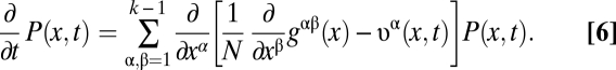The matrix g^αβ(x) characterizes genetic drift, and the evolution rates contain the contributions of mutations and time-dependent selection with coefficients s_β(x, t) (for details, see SI Text). A stationary neutral process with mutation rates μ_α^β satisfying the detailed balance conditions μ_α^β/μ_β^α = p₀^β/p₀^α can be shown to have an asymptotic equilibrium distribution P₀(x) in the regime for genotypes or for allele frequencies in linkage equilibrium (SI Text). Under the same conditions, the corresponding process in any time-independent fitness landscape F(x) has an equilibrium distribution P_eq(x) of the form (Eq. 2), as shown by inspection of the diffusion equation (Eq. 6).

Derivation of the Fitness-Flux Theorem.

Consider the ensemble of population histories x = (x₀, …, x_n) with a sufficiently dense set of observation times t_i = t₀ + iδ (i = 0, …, n). For a generic diffusion process of the form (Eq. 6), this ensemble is characterized by a probability distribution of histories, which determines the frequency distribution and has the normalization . Using standard methods of statistical mechanics, we compute the conditional probability of a history for a given initial state, , and its neutral counterpart G₀(x). These enjoy the relation with scalar products v² and m² defined in SI Text. We now consider the reverse history x^T = (x₀^T, …, x_n^T), which is given by x_i^T = x_n–i (i = 0, …, n), and, by definition, evolves in the time-reversed fitness landscape F^T(x, t) = F(x, t_n – t + t₀) (Fig. 1). Using the method of refs 32–34, we compare the conditional probabilities of original and reverse history (Eq. 7),

Inserting the definition of the relative log likelihood, , then yields Eq. 3, and the theorem (Eq. 4) follows by summation over all histories. For a time-dependent population size parameterized in terms of a reference size, N(t) = ζ(t)N₀, and the scaled fitness flux defined as , the identity (Eq. 4) remains valid in very good approximation for low mutation rates. This is shown by an inhomogeneous rescaling of time by a factor 1/ζ(t) in the evolution equation (Eq. 6). A more detailed derivation of the theorem is given in SI Text.

Fisher’s Theorem.

In the strong-selection limit of the evolutionary process (Eq. 6), the evolution of a polymorphic population is dominated (except for small frequencies of x < 1/Ns) by its most probable history, which follows the deterministic evolution equation . Hence, its fitness flux Φ_* increases at a rate , which is the fitness variance in the population (SI Text). Fisher’s theorem is the projection of this identity from genotype frequencies to gene-allele frequencies.

References

- 1.Fisher RA. In: The Genetical Theory of Natural Selection: A Complete Variorum Edition. Bennet H, editor. Oxford, UK: Oxford University Press; 2000. [Google Scholar]
- 2.Price GR. Selection and covariance. Nature. 1970;227:520–521. doi: 10.1038/227520a0. [DOI] [PubMed] [Google Scholar]
- 3.Kimura M. On the change of population fitness by natural selection. Heredity. 1958;12:145–167. [Google Scholar]
- 4.Iwasa Y. Free fitness that always increases in evolution. J Theor Biol. 1988;135:265–281. doi: 10.1016/s0022-5193(88)80243-1. [DOI] [PubMed] [Google Scholar]
- 5.Nagylaki T. Rate of evolution of a character without epistasis. Proc Natl Acad Sci USA. 1989;86:1910–1913. doi: 10.1073/pnas.86.6.1910. [DOI] [PMC free article] [PubMed] [Google Scholar]
- 6.Sato K, Ito Y, Yomo T, Kaneko K. On the relation between fluctuation and response in biological systems. Proc Natl Acad Sci USA. 2003;100:14086–14090. doi: 10.1073/pnas.2334996100. [DOI] [PMC free article] [PubMed] [Google Scholar]
- 7.Vlad MO, et al. Fisher’s theorems for multivariable, time- and space-dependent systems, with applications in population genetics and chemical kinetics. Proc Natl Acad Sci USA. 2005;102:9848–9853. doi: 10.1073/pnas.0504073102. [DOI] [PMC free article] [PubMed] [Google Scholar]
- 8.Rice SH. A stochastic version of the Price equation reveals the interplay of deterministic and stochastic processes in evolution. BMC Evol Biol. 2008;8:262. doi: 10.1186/1471-2148-8-262. [DOI] [PMC free article] [PubMed] [Google Scholar]
- 9.Wright S. Proceedings of the Sixth International Congress on Genetics. 1932. The roles of mutation, inbreeding crossbreeding and selection in evolution; pp. 356–366. [Google Scholar]
- 10.Ohta T. Population size and rate of evolution. J Mol Evol. 1972;1:305–314. [PubMed] [Google Scholar]
- 11.Gillespie JH. Substitution processes in molecular evolution. I. Uniform and clustered substitutions in a haploid model. Genetics. 1993;134:971–981. doi: 10.1093/genetics/134.3.971. [DOI] [PMC free article] [PubMed] [Google Scholar]
- 12.Kussell E, Leibler S. Phenotypic diversity, population growth, and information in fluctuating environments. Science. 2005;309:2075–2078. doi: 10.1126/science.1114383. [DOI] [PubMed] [Google Scholar]
- 13.Mustonen V, Lässig M. Adaptations to fluctuating selection in Drosophila. Proc Natl Acad Sci USA. 2007;104:2277–2282. doi: 10.1073/pnas.0607105104. [DOI] [PMC free article] [PubMed] [Google Scholar]
- 14.Mustonen V, Lässig M. Molecular evolution under fitness fluctuations. Phys Rev Lett. 2008;100:108101. doi: 10.1103/PhysRevLett.100.108101. [DOI] [PubMed] [Google Scholar]
- 15.Mustonen V, Lässig M. From fitness landscapes to seascapes: Non-equilibrium dynamics of selection and adaptation. Trends Genet. 2009;25:111–119. doi: 10.1016/j.tig.2009.01.002. [DOI] [PubMed] [Google Scholar]
- 16.Weinreich DM, Watson RA, Chao L. Perspective: Sign epistasis and genetic constraint on evolutionary trajectories. Evolution. 2005;59:1165–1174. [PubMed] [Google Scholar]
- 17.Weinreich DM, Delaney NF, Depristo MA, Hartl DL. Darwinian evolution can follow only very few mutational paths to fitter proteins. Science. 2006;312:111–114. doi: 10.1126/science.1123539. [DOI] [PubMed] [Google Scholar]
- 18.Desai MM, Fisher DS, Murray AW. The speed of evolution and maintenance of variation in asexual populations. Curr Biol. 2007;17:385–394. doi: 10.1016/j.cub.2007.01.072. [DOI] [PMC free article] [PubMed] [Google Scholar]
- 19.Poelwijk FJ, Kiviet DJ, Weinreich DM, Tans SJ. Empirical fitness landscapes reveal accessible evolutionary paths. Nature. 2007;445:383–386. doi: 10.1038/nature05451. [DOI] [PubMed] [Google Scholar]
- 20.de Visser JAGM, Park SC, Krug J. Exploring the effect of sex on empirical fitness landscapes. Am Nat. 2009;174(Suppl 1):S15–S30. doi: 10.1086/599081. [DOI] [PubMed] [Google Scholar]
- 21.Barrick JE, et al. Genome evolution and adaptation in a long-term experiment with Escherichia coli. Nature. 2009;461:1243–1247. doi: 10.1038/nature08480. [DOI] [PubMed] [Google Scholar]
- 22.Kerr B, Riley MA, Feldman MW, Bohannan BJM. Local dispersal promotes biodiversity in a real-life game of rock-paper-scissors. Nature. 2002;418:171–174. doi: 10.1038/nature00823. [DOI] [PubMed] [Google Scholar]
- 23.Sinervo B, Lively CM. The rock paper scissors game and the evolution of alternative male strategies. Nature. 1996;380:240–243. [Google Scholar]
- 24.McDonald JH, Kreitman M. Adaptive protein evolution at the Adh locus in Drosophila. Nature. 1991;351:652–654. doi: 10.1038/351652a0. [DOI] [PubMed] [Google Scholar]
- 25.Price GR. Fisher’s ‘fundamental theorem’ made clear. Ann Hum Genet Lond. 1972;36:129–140. doi: 10.1111/j.1469-1809.1972.tb00764.x. [DOI] [PubMed] [Google Scholar]
- 26.Ewens WJ. An interpretation and proof of the fundamental theorem of natural selection. Theor Popul Biol. 1989;36:167–180. doi: 10.1016/0040-5809(89)90028-2. [DOI] [PubMed] [Google Scholar]
- 27.Kimura M. Stochastic processes and distribution of gene frequencies under natural selection. Cold Spring Harb Symp Quant Biol. 1955;20:33–53. doi: 10.1101/sqb.1955.020.01.006. [DOI] [PubMed] [Google Scholar]
- 28.Halpern AL, Bruno WJ. Evolutionary distances for protein-coding sequences: Modeling site-specific residue frequencies. Mol Biol Evol. 1998;15:910–917. doi: 10.1093/oxfordjournals.molbev.a025995. [DOI] [PubMed] [Google Scholar]
- 29.Mustonen V, Kinney J, Callan CG, Jr, Lässig M. Energy-dependent fitness: A quantitative model for the evolution of yeast transcription factor binding sites. Proc Natl Acad Sci USA. 2008;105:12376–12381. doi: 10.1073/pnas.0805909105. [DOI] [PMC free article] [PubMed] [Google Scholar]
- 30.Berg J, Willmann S, Lässig M. Adaptive evolution of transcription factor binding sites. BMC Evol Biol. 2004;4:42. doi: 10.1186/1471-2148-4-42. [DOI] [PMC free article] [PubMed] [Google Scholar]
- 31.Jarzynski C. Nonequilibrium equality for free energy differences. Phys Rev Lett. 1997;78:2690. [Google Scholar]
- 32.Crooks GE. Entropy production fluctuation theorem and the nonequilibrium work relation for free energy differences. Phys Rev E. 1999;60:2721–2726. doi: 10.1103/physreve.60.2721. [DOI] [PubMed] [Google Scholar]
- 33.Seifert U. Entropy production along a stochastic trajectory and an integral fluctuation theorem. Phys Rev Lett. 2005;95:040602. doi: 10.1103/PhysRevLett.95.040602. [DOI] [PubMed] [Google Scholar]
- 34.Chernyak VY, Chertkov M, Jarzynski C. Path-integral analysis of fluctuation theorems for general Langevin processes. J Stat Mech. 2006;8:080001. [Google Scholar]
- 35.Burch CL, Chao L. Evolution by small steps and rugged landscapes in the RNA Virus φ6. Genetics. 1999;151:921–927. doi: 10.1093/genetics/151.3.921. [DOI] [PMC free article] [PubMed] [Google Scholar]
- 36.Sella G, Hirsh AE. The application of statistical physics to evolutionary biology. Proc Natl Acad Sci USA. 2005;102:9541–9546. doi: 10.1073/pnas.0501865102. [DOI] [PMC free article] [PubMed] [Google Scholar]
- 37.Andolfatto P. Adaptive evolution of non-coding DNA in Drosophila. Nature. 2005;437:1149–1152. doi: 10.1038/nature04107. [DOI] [PubMed] [Google Scholar]
- 38.Macpherson JM, Sella G, Davis JC, Petrov DA. Genomewide spatial correspondence between nonsynonymous divergence and neutral polymorphism reveals extensive adaptation in Drosophila. Genetics. 2007;177:2083–2099. doi: 10.1534/genetics.107.080226. [DOI] [PMC free article] [PubMed] [Google Scholar]
- 39.Peliti L. Introduction to the statistical theory of Darwinian evolution. 1997. cond-mat/9712027. [Google Scholar]
- 40.Drossel B. Biological evolution and statistical physics. Advances in Physics. 2001;50:209–295. [Google Scholar]
- 41.Kimura M. The Neutral Theory of Molecular Evolution. Cambridge, UK: Cambridge University Press; 1983. [Google Scholar]
Associated Data
This section collects any data citations, data availability statements, or supplementary materials included in this article.